Fault Severity Monitoring of Rolling Bearings Based on Texture Feature Extraction of Sparse Time–Frequency Images


1
School of Mechanical Electronic and Information Engineering, China University of Mining and Technology, Beijing 100083, China
2
School of Information and Communication Engineering, University of Electronic Science and Technology of China, Chengdu 610054, China
3
School of Physics and Information Engineering, Minnan Normal University, Zhangzhou 363000, China
4
School of Mechanical-Electrical Engineering, North China Institute of Science and Technology, Yanjiao 101601, China
*
Author to whom correspondence should be addressed.
Appl. Sci. 2018, 8(9), 1538; https://doi.org/10.3390/app8091538
Submission received: 21 July 2018
/
Revised: 16 August 2018
/
Accepted: 21 August 2018
/
Published: 3 September 2018
(This article belongs to the Special Issue Fault Detection and Diagnosis in Mechatronics Systems)
Abstract
:Rolling bearings are important components of rotating machines. For their preventive maintenance, it is not enough to know whether there is any fault or the fault type. For an effective maintenance, a fault severity monitoring needs to be conducted. Currently, the bearing fault diagnosis method based on time–frequency image (TFI) recognition is attracting increasing attention. This paper contributes to the ongoing investigation by proposing a new approach for the fault severity monitoring of rolling bearings based on the texture feature extraction of sparse TFIs. The first and main step is to obtain accurate TFIs from the vibration signals of rolling bearings. Traditional time–frequency analysis methods have disadvantages such as low resolution and cross-term interference. Therefore, the TFIs obtained cannot satisfactorily express the time–frequency characteristics of bearing vibration signals. To solve this problem, a sparse time–frequency analysis method based on the first-order primal-dual algorithm (STFA-PD) was developed in this paper. Unlike traditional time–frequency analysis methods, the time–frequency analysis model of the STFA-PD method is based on the theory of sparse representation, and is solved using the first-order primal-dual algorithm. For employing the sparse constraint in the frequency domain, the STFA-PD obtains a higher time–frequency resolution and is free from cross-term interference, as the model is based on a linear time–frequency analysis method. The gray level co-occurrence matrix is then employed to extract texture features from the sparse TFIs as input features for classifiers. Vibration signals of rolling bearings with different fault severity degrees are used to validate the proposed approach. The experimental results show that the developed STFA-PD outperforms traditional time–frequency analysis methods in terms of the accuracy and effectiveness for the fault severity monitoring of rolling bearings.
1. Introduction
Rolling bearings are important and vulnerable components widely used in rotating machinery. The running state of rolling bearings significantly affects the performance, safety, and reliability of the overall machinery [1,2,3]. Therefore, the state detection and fault diagnosis for rolling bearings have important practical significance. As bearing failure is a dynamic process, it is insufficient to know whether there is any fault or the fault type for the preventive maintenance of bearings in engineering applications. Determining the failure evolution process and accurately monitoring the fault severity are paramount for an effective bearing maintenance [4,5,6]. Consequently, the fault severity monitoring of rolling bearings is becoming increasingly important [7,8].
It would be instructive and practical to describe overall modes of bearing failure first. Bearing failure is not always due to vibration. There are many reasons for bearing failure. In fact, in most cases, the initiating source of failure is lubrication. The lack of a lubricant film between the rolling element and races will result in increased friction and wear. These conditions lead to generated heat, and thus, surface scoring and scuffing and even bearing dimensional instability. Of course, these can lead to vibration; however, by the time this occurs, the bearing is really in a failed state and needs to be replaced. There are three sources of failure for which the timely monitoring of vibrations is effective for prevention. The first one is poor assembly or loss of preload or interference fit, which leads to out-of-balance rotation and gradually excessive cage responses [9]. The second one is the variable compliance vibration which is inherent to ball and rolling element bearings [10,11]. Any amplitude increase at this frequency can lead to premature resonance and occurs with loss of preload or radial interference fit. The last one is increased contact loads, which cause fatigue spalling as the result of sub-surface stresses [12], leading to pits, cracks, etc. on the rolling surfaces. In this study, we focus on monitoring the fault severity of rolling bearings caused by the latter source of failure using vibration signals.
The first step in fault severity monitoring is obtaining the appropriate signals. As discussed before, the vibration signal is suitable for monitoring the fault severity. Moreover, compared to signals of temperature, sound, stress, and strain, a vibration signal carries considerable information regarding bearing health conditions and is easy to collect. Thereafter, the key step is to process the vibration signals. Time-domain and frequency-domain signal analysis methods, such as time-domain feature extraction, fast Fourier transform (FFT), and envelope analysis, were used to process vibration signals in the past [13,14,15,16]. However, the fault vibration signals of rolling bearings often exhibit nonlinear and non-stationary characteristics, making it difficult to accurately recognize the fault severity degree of bearings only in the time domain or in the frequency domain. Some non-stationary signal processing methods were developed. For example, the cyclostationarity method is a commonly used method to process non-stationary signals and was applied to some extent in the field of fault diagnosis of rotating machinery in the past few years [17,18,19]. Compared to the methods mentioned above, the time–frequency analysis methods are more effective when dealing with nonlinear and non-stationary signals, because they can accurately describe the local time–frequency characteristics of non-stationary signals by revealing the constituent frequency components and their time-variation characteristics. In fact, these methods are widely used in the field of mechanical fault diagnosis [20,21,22]. To date, the traditional time–frequency analysis methods, which are also commonly used methods, can be roughly divided into two classes [20]: linear time–frequency analysis methods, such as short-time Fourier transform (STFT), Gabor transform [23,24], wavelet transform (WT), and the S transform (ST); and bilinear/quadratic time–frequency analysis represented by the Wigner–Ville distribution (WVD) [22,25,26,27,28,29]. In fact, WT is a time-scale method, but there is a relationship between scale and frequency. Thus, WT can be used to conduct a time–frequency analysis for a signal. In addition, WT is also used to decompose a vibration signal into its wavelet components and choose the components that are related to the specific desired frequencies [30]. However, a substantial amount of useful information may be lost.
Governed by the Heisenberg uncertainty principle, the time and frequency resolutions of linear time–frequency analysis methods cannot simultaneously achieve the desired optimum effects. As a result, the time–frequency resolution is often low. On the contrary, bilinear time–frequency analysis methods have a higher time–frequency resolution. However, their time–frequency distributions are inevitably subjected to cross-term interference, which is not the case with linear time–frequency representations [20].
In recent years, the sparse representation (SR) theory attracted widespread attention and was applied to many fields, particularly to signal and image processing [31,32,33,34,35,36]. With the application of SR theory in the field of time–frequency analysis, a new time–frequency representation (TFR) model based on SR and STFT emerged [37,38]. The time–frequency analysis problem is essentially converted into a sparse optimization problem based on the L0-norm constraint. The time–frequency distribution with higher concentration and resolution can be obtained by solving the sparse optimization problem. Moreover, as the model is based on the STFT framework, there is no cross-item interference. As a result, this model can better describe the time–frequency characteristics of the signals and was successfully applied to the analysis of non-stationary signals, such as seismic and radar signals [39,40]. In this paper, this model was applied to conduct the time–frequency analysis of bearing vibration signals. However, the optimization problem with respect to this model is an L0-norm minimization problem, i.e., a non-convex optimization problem, which is NP-hard and very difficult to solve. To address this issue, a first-order primal-dual algorithm-based sparse time–frequency analysis method (STFA-PD) was developed. Firstly, the non-convex optimization problem of L0-norm was relaxed to an L1-norm minimization problem using a convex relaxation technique. Secondly, the first-order primal-dual algorithm was employed to solve the problem [41,42].
Several time–frequency images (TFIs) reflecting the bearing condition can be obtained by conducting the time–frequency analysis of vibration signals. Currently, there are two types of bearing condition recognition methods based on TFIs [43,44]. The first one is an artificial recognition method performed by skilled experts. This method relies heavily on individual experience and skill level and has low accuracy and efficiency for bearing condition recognition. The other is an automatic classification using computers, which is attracting increasing attention. Although TFIs can effectively characterize the local time–frequency properties of rolling bearing vibration signals, they cannot be directly used as features for an automatic classification, because the data dimensions of TFIs are too numerous for such a classification. Therefore, image dimensionality reduction and feature extraction need to be conducted before classification. Some algebraic feature extraction methods, such as two-direction two-dimensional principal component analysis (TD-2DPCA) [45], two-direction two-dimensional linear discriminant analysis (TD-2DLDA) [46], and two-dimensional non-negative matrix factorization (2DNMF) [43], were proposed for the dimensionality reduction of TFIs. The low-dimensional features obtained through dimensionality reduction are directly used for automatic classification. However, as the horizontal distribution of the frequency properties in TFIs changes with time, the features will be inevitably affected by the influence of the time-domain truncation. As a result, even the TFIs with the same fault severity may have completely different features.
Bearing vibration signals of different states can be used to express different characteristics in the time–frequency domain, resulting in TFIs with different textures. Additionally, the texture features can be expressed as global statistics of local features, which has little to do with the changes in the horizontal distribution with time. Therefore, texture-feature-based image classification can be used to distinguish the fault severity degrees of bearings. The most widely used texture descriptor for image recognition is the gray level co-occurrence matrix (GLCM), proposed by Haraclick et al. [47] in 1973, as it can accurately describe the roughness, repetition direction, and complexity of the texture of an image. GLCM is a square matrix. GLCMs with different parameters can be easily obtained from a single image, while many statistical features can be easily obtained from each GLCM. Compared to GLCM, the statistical features are more convenient for classification. Consequently, GLCM-based texture features, i.e., statistical features, can be extracted from TFIs to obtain fault severity information.
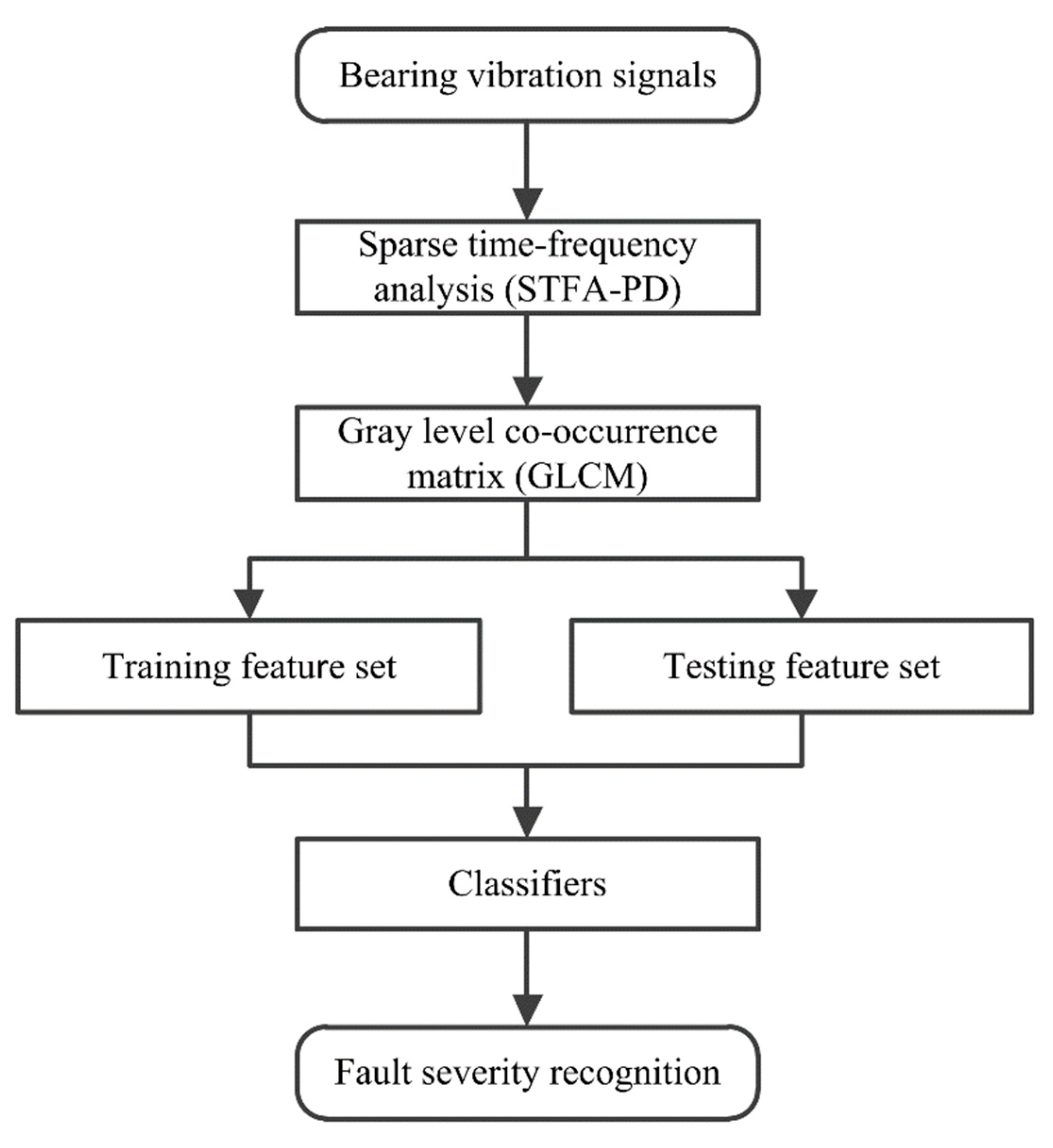
A new approach for the fault severity monitoring of rolling bearings based on the texture feature extraction of sparse TFIs is proposed in this paper. The novelty is that a new time–frequency analysis method, named STFA-PD, was developed for analyzing the bearing vibration signal. A high-quality TFI without the cross-term interference, which we call sparse TFI, can be obtained from the vibration signal using the STFA-PD method. Thereafter, the GLCM can be used to extract the texture features from sparse TFIs as the input features for classifiers. Finally, the fault severity recognition can be realized. Figure 1 shows a flowchart of the proposed bearing fault severity monitoring approach.
The rest of this paper is organized as follows: in Section 2, the STFA-PD is described in detail, including the establishment of the model and the algorithm solution to the sparse optimization problem. In addition, the superiority of the STFA-PD is verified using a simulated signal. The calculation of GLCM and its statistical features are briefly reviewed in Section 3. In Section 4, the vibration signals of the rolling bearings with different fault severity degrees are used to validate the proposed approach. Finally, the conclusions of this investigation are given in Section 5.
2. First-Order Primal-Dual Algorithm-Based Sparse Time–Frequency Analysis
2.1. Model of Sparse Time–Frequency Analysis
The short-time Fourier transform (STFT) is one of the earliest and most widely used time–frequency analysis methods. The basic idea of the STFT can be summarized as described below. A short time window is added to the desired signal, and the local Fourier spectrum of the windowed signal is calculated. By sliding the window with respect to time, the time–frequency analysis of the signal can be carried out [20,48]. The STFT of the continuous-time signal can be defined as follows:
where is the sliding window function.
Correspondingly, for a discrete signal of period N, where , the discrete STFT can be defined as follows:
where , and .
According to Equation (1), the STFT of the continuous-time signal can be regarded as a Fourier transform (FT) of the windowed signal . On the contrary, when and window functions are given, the original signal can be directly recovered by inverse Fourier transform (IFT), which can be represented as follows:
Correspondingly, for the windowed signal of at time , the discrete STFT can be defined as follows:
The vector form of can be expressed as follows:
where and are the windowed signal and Fourier spectrum at time , respectively; is the inverse Fourier transform matrix; and , where .
The short-time truncated sub-signal can be given as follows:
where is the short-time truncated sub-signal, is the sliding window at time , and the sliding window at time is the circular shift of with the column values shifted to right by one.
In Equation (6), is a partial Fourier matrix, and its columns may be highly correlated, where this cannot guarantee the uniqueness of the solution of . The windowed signal at time is sparse in the frequency domain. Inspired by SR theory, the special spectrum can be easily obtained by adding the sparse constraint to fit the sparse prior knowledge of the spectrum. The sparse constraint problem can be modeled as Equation (7).
where denotes the L0-norm. By comparing Equations (6) and (7), we find that plays the role of a dictionary of SR. Considering that the L0-norm minimization problem is NP-hard, the L1-norm is generally approximated to the L0-norm, i.e., the convex relaxation is considered an L1-norm minimization problem, or an interference in practical situations. Therefore, we can estimate the spectrum by solving the sparse constraint problem modeled as Equation (8).
where denote the L1-norm, is the estimated signal spectrum at time , and is a user-specified parameter related to noise.
The sparse time–frequency spectrum can be finally obtained by solving a group of optimization problems, Equation (8), for all . The group of optimization problems is called the sparse time–frequency model.
2.2. Solution of the Model Based on the First-Order Primal-Dual Algorithm
As the model is a set of convex optimization problems with constraints, it can be rewritten as an unconstrained optimization problem, i.e., Equation (9), which is convenient for solving, as follows:
where is the sparse term, is the sparse coefficient, and is the fidelity term.
Assuming and , according to the first-order primal-dual algorithm, the solution can be trivially given by the following sequence of convex problems:
where is the unit matrix, and are resolvent operators, is the convex conjugate of , is the convex conjugate function of , is the dual variable, and is the convex set defined as follows:
The resolvent operator with respect to can be obtained as follows:
As is the indicator function for a convex set, the resolvent operator with respect to reduces to pointwise Euclidean projectors:
The resolvent operator with respect to can be expressed as follows:
The resolvent operator with respect to is a simple convex quadratic programming problem, the solution to which is given as follows:
The sparse time–frequency spectrum of the signal can be finally obtained by solving a group of optimization problems, such as Equation (9), using the first-order primal-dual algorithm for .
The pseudocode of the STFA-PD is summarized in Algorithm 1.
| Algorithm 1. Sparse time–frequency analysis method based on the first-order primal-dual algorithm (STFA-PD) |
| Input: |
| Output: |
| Initialize: |
| 1: For do |
| 2: For do |
| 3: |
| 4: |
| 5: |
| 6: End For |
| 7: End for |
| 8: Return as |
2.3. Simulation Analysis
To validate the effectiveness and superiority of the STFA-PD, a multi-component simulated signal, defined by Equation (16), was employed:
where was a sinusoidal signal and both and were nonlinear frequency-modulated signals. The sampling frequency was set to 1000 Hz, and the sample length was 1 s.
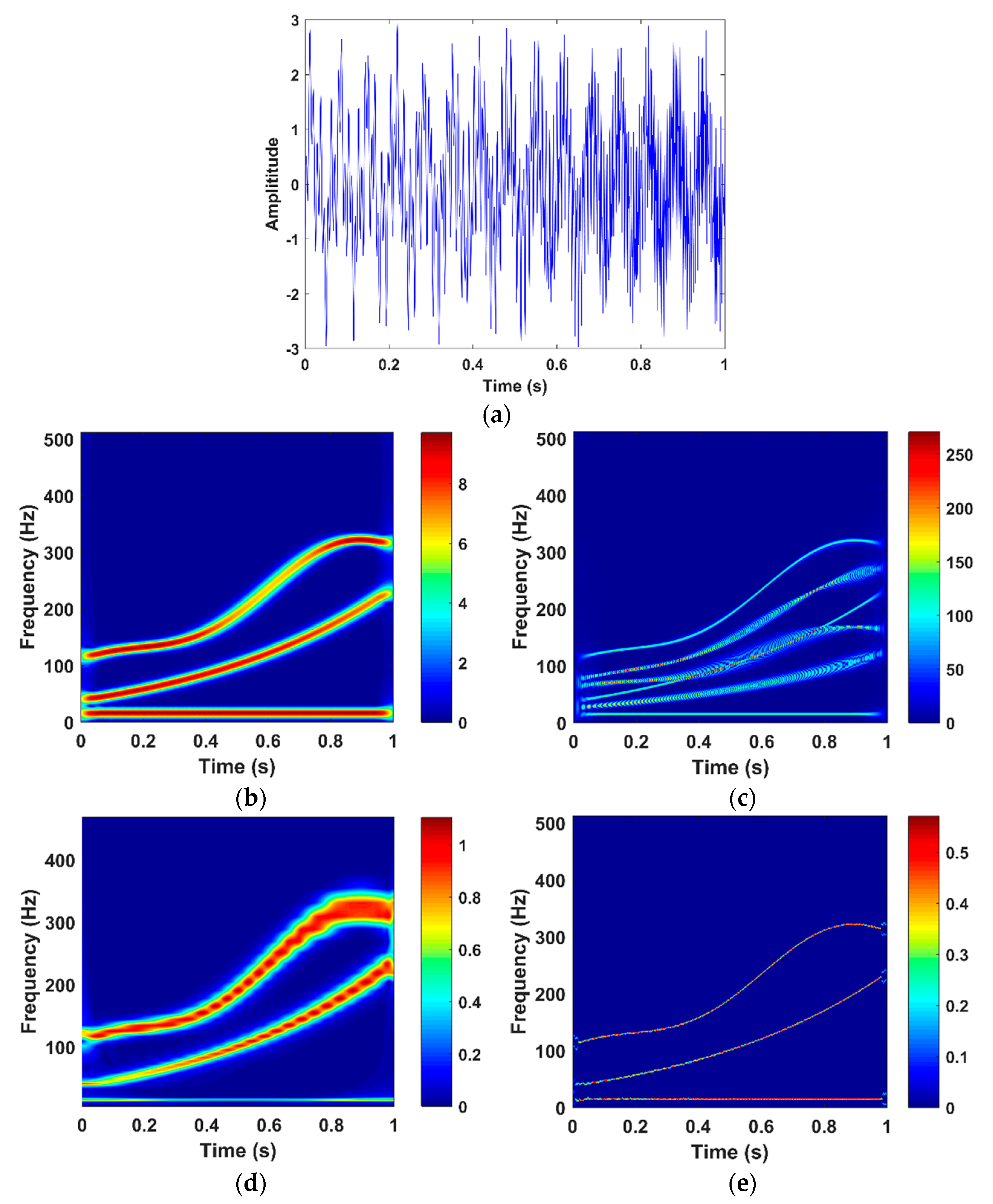
Figure 2a shows the time-domain waveform of the simulated signal , which was a non-stationary signal with a frequency that varied with time. Figure 2b,e show the TFIs obtained using the STFT, pseudo WVD (PWVD), WT, and the STFA-PD. In this study, the bump mother wavelet was used in WT of the simulated signal, as well as bearing vibration signals.
Figure 2b shows that the resolution of the traditional STFT was low either in the lower frequency band or in the higher frequency band, and the time–frequency distribution of the signal was not accurately reflected. By contrast, the TFI obtained using the PWVD was good in terms of the time–frequency resolution, but suffered from cross-term interferences, and thus, did not precisely reflect the time–frequency characteristics of the signal, as shown in Figure 2c. As shown in Figure 2d, the TFI obtained using the WT had a good time–frequency resolution in the lower frequency band, but a poor resolution in the higher frequency band. As the WT was essentially a type of time-scale transform and as there was no good correspondence between the scale and the frequency of the signal, the WT did not accurately express the time-based variations in the frequency of each component of the signal. Figure 2e shows the TFI obtained using the STFA-PD method. Comparing Figure 2e with Figure 2b–d, we see that the STFA-PD method had higher time–frequency concentration and resolution than the other methods.
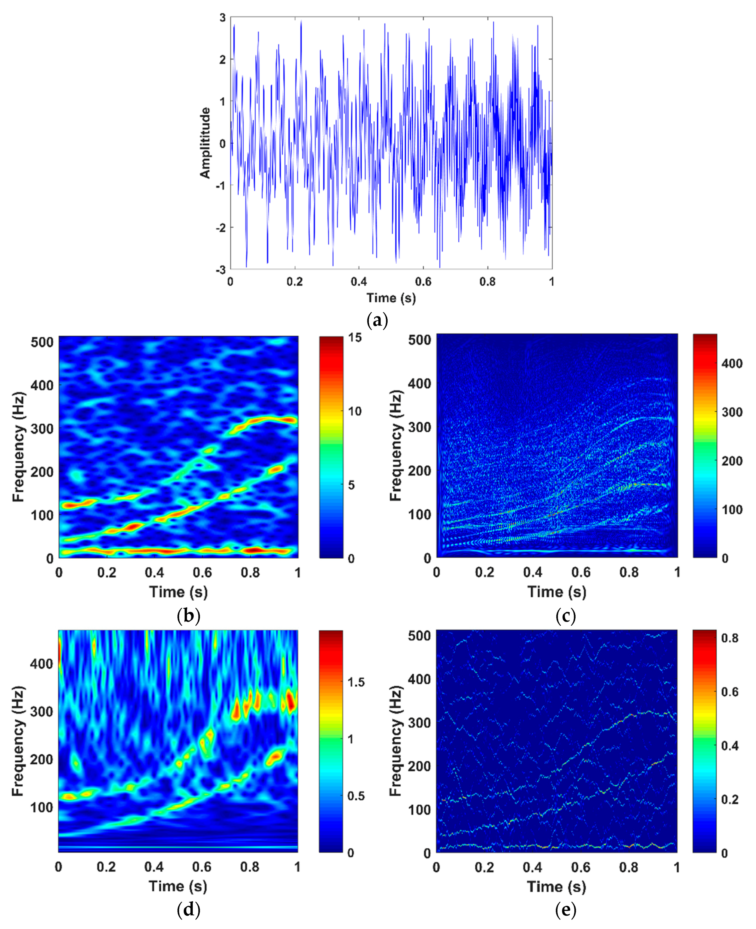
To validate the denoising performance of the STFA-PD method, the Gaussian white noise was artificially added to the simulated signal . The noisy signal was denoted as . Figure 3a shows the time-domain waveform of the noisy signal with the signal-to-noise ratio (SNR) of −2 dB. Figure 3b–e show the TFIs obtained using STFT, PWVD, WT, and STFA-PD. It can be seen there were different degrees of noise interferences in the TFIs. As displayed in Figure 3c, The TFI obtained by PWVD seemed more sensitive to the noise than others. The time-frequency characteristic of the signal was almost masked by the noise and cross-term interferences. From Figure 3e, we can find that The TFI obtained by STFA-PD still had a high time-frequency resolution even if there was a high level of noise.
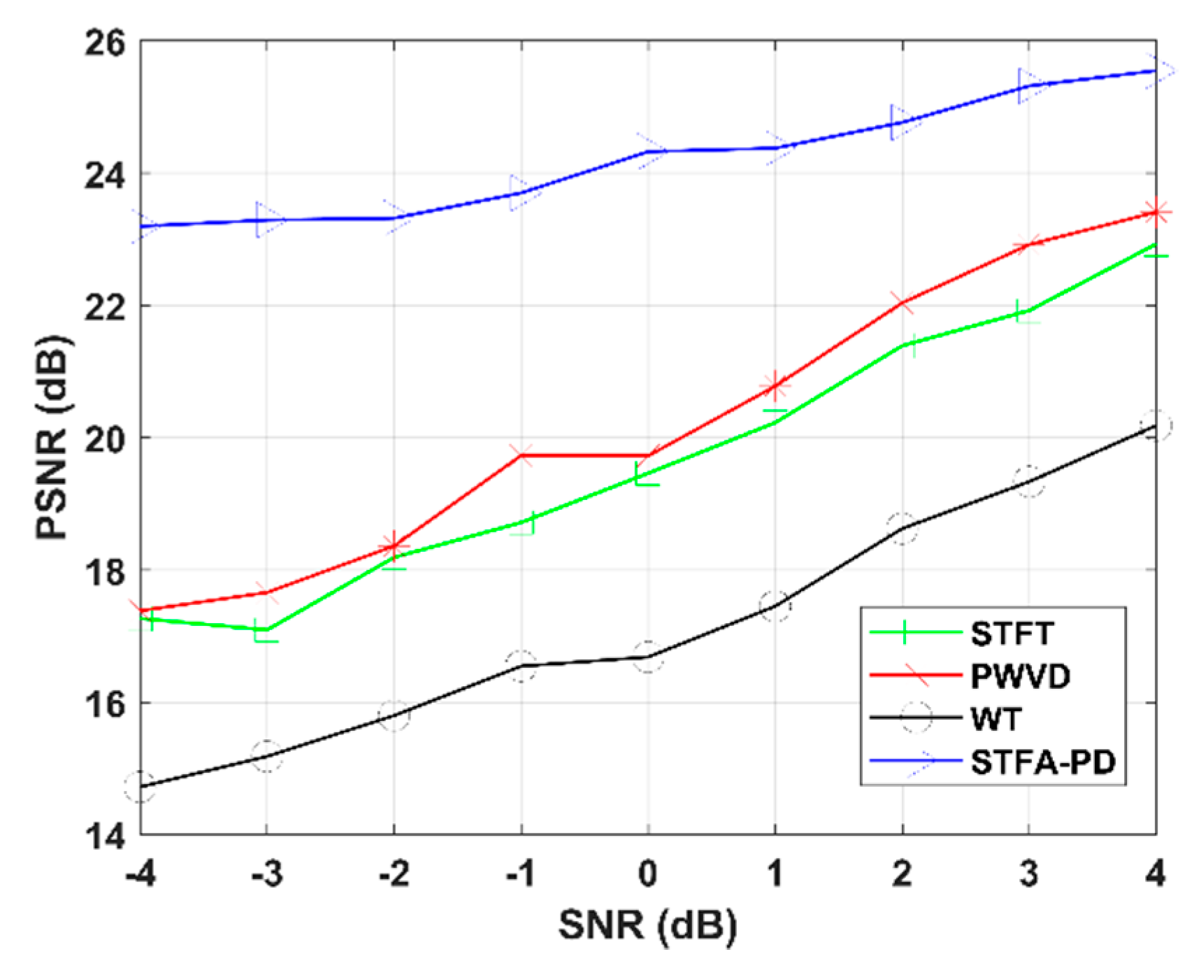
To further quantitatively analyze and evaluate the denoising performance of the STFA-PD method, the peak signal-to-noise ratio (PSNR) was adopted as a denoising performance evaluation measurement. The PSNR is defined as follows:
where is the TFI of the simulated signal , and is the TFI of the noisy signal ; the bigger the PSNR is, the closer and are; is the maximal value of . Figure 4 shows the PSNR values obtained by different methods (i.e., STFT, PWVD, WT, and the proposed STFA-PD method) at different SNR levels. It can be seen the STFA-PD method obtained bigger a PSNR value than the other three methods, which meant the STFA-PD method was better in terms of denoising performance than others. Moreover, it can also be seen that the PSNR value became smaller along with the SNR getting lower. However, the PSNR value obtained by STFA-PD fell more slowly than others. Even at a low SNR of −4 dB, the PSNR value obtained by STFA-PD was still high.
3. GLCM-Based Image Texture Features
3.1. Brief Introduction of GLCM
The texture is formed by the repeated appearance of the gray distribution in spatial positions. Thus, there will be a certain gray relationship between two pixels separated by a certain distance in the image space, which is the spatial correlation characteristic of gray in the image. In image recognition, the GLCM is a commonly used method for image texture analysis [47,49]. By studying the spatial correlation characteristics of gray levels in the image, the GLCM can be used to accurately describe image texture features. The GLCM can be obtained by counting the co-occurrence frequency of gray levels of a pair of pixels with a certain positional relationship in the two-dimensional (2D) space of a gray image.
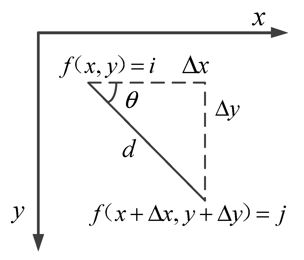
Figure 5 shows the calculation schematic of the GLCM. Given a pixel pair with gray level and , the co-occurrence frequency of the pixel pairs can be defined as follows:
where denotes the total number of pixel pairs satisfying the conditions, is the gray level, are the coordinates of the pixel with gray level , are the coordinates of the pixel with gray level , and are the position offsets in the horizontal and vertical directions, respectively, is the generation step, and is the direction of generation.
The matrix composed of frequency with specified values of and is the GLCM, an square matrix. Four GLCMs with are generally used for texture analysis.
The generation step is determined by the horizontal and vertical offsets . Therefore, the GLCMs of an image can change with respect to . The value of should be selected according to the characteristics of the periodic distribution of texture. For thinner and more slowly changing texture images, lower values should be taken, and higher values should be chosen for images of textures that change quickly.
3.2. Statistical Features of GLCM
For the texture analysis of an image, the GLCM is often not directly used as the texture features of the image. In fact, the statistical features extracted from the GLCM are used as the texture features.
Before extracting the statistical features from the GLCM, the frequency should be normalized to co-occurrence probability as follows:
Haraclick et al. [47] suggested many statistical features, such as maximum probability, entropy, contrast, correlation, energy, and inverse differential moment. Three of them were calculated here: entropy, contrast, and energy. This is because the results of an experiment conducted by Baraldi and Parmiggiani [50] showed that these statistical features are suitable for effective classification and image recognition.
Entropy is used to characterize the information capacity of an image and to characterize the complexity or non-uniformity of image texture. The entropy is highest when the image is full of texture and lowest when there is no texture:
Contrast is a measure of the degree of texture clarity, and it is expressed as in Equation (20). The deeper the texture groove, the greater the contrast in the image, and vice versa. For example, the contrast of a constant image is zero, as there is only a single non-zero element in the GLCM.
Energy, also known as the angular second moment (ASM), can be defined as follows:
It characterizes the uniformity of the gray distribution of the image texture, and can reflect its roughness. When image texture is coarser, i.e., when the frequency distribution in a TFI is more concentrated, the energy is greater and vice versa.
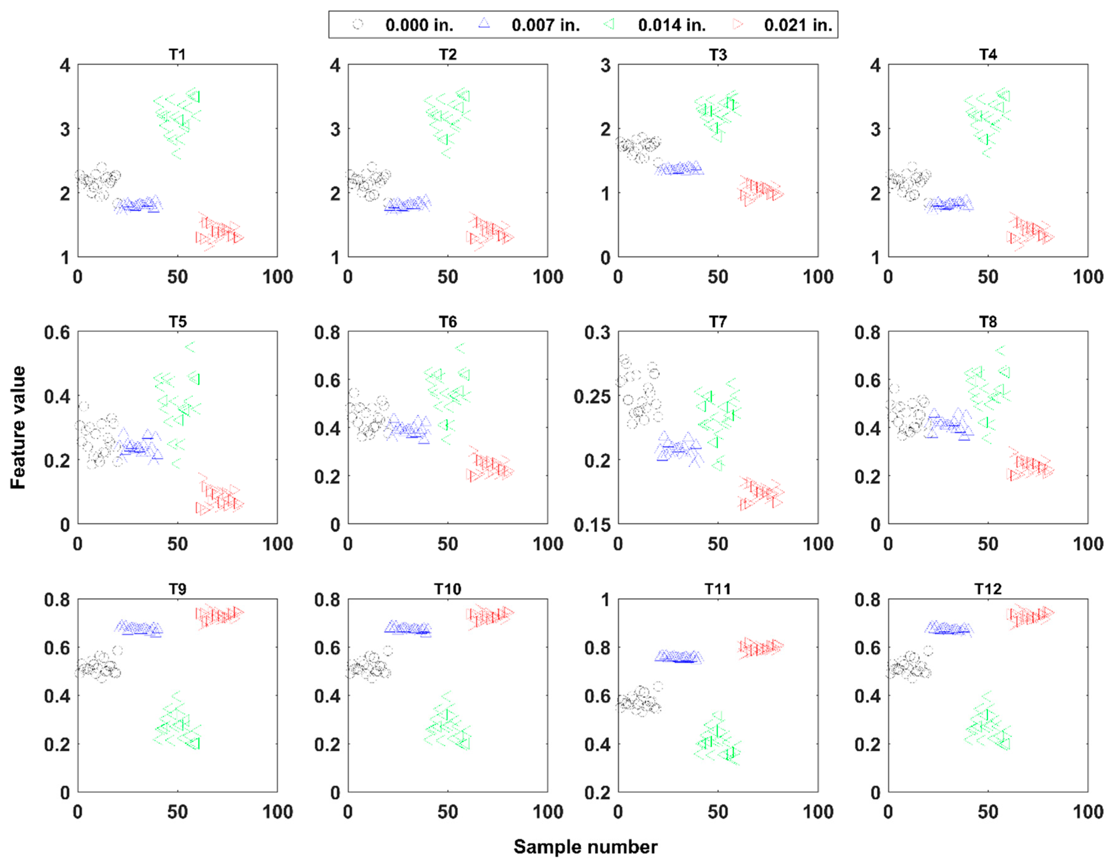
In this study, four GLCMs with were employed. We extracted three types of statistical features from the four GLCMs as texture features for characterizing the TFIs of the vibration signals. The 12 features were expressed as T1, T2, ····, T12, where T1, T2, T3, and T4 represent entropy features; T5, T6, T7, and T8 represent contrast features; and T9, T10, T11, and T12 represent energy features of the four GLCMs.
4. Experimental Validation and Discussion
4.1. Experimental Data and Setup
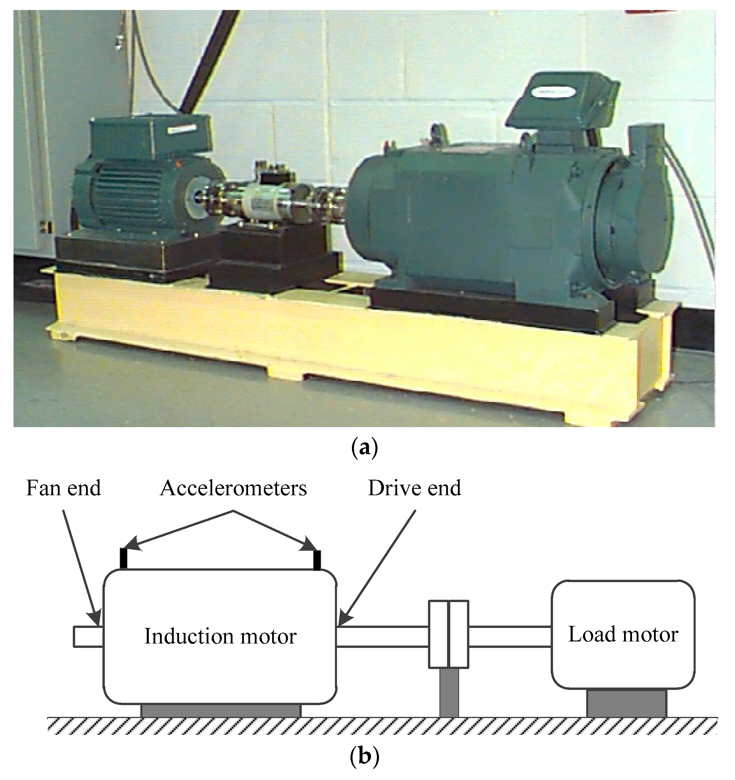
The bearing data used in this study were obtained from the Bearing Data Center of the Electrical Engineering Laboratory at the Case Western Reserve University (CWRU) [51,52,53]. Figure 6 shows the bearing test stand and its structural diagram. The test stand included a 2 horsepower motor, a torque transducer/encoder, a dynamometer, and control electronics. The motor bearings were seeded with single-point faults using electro-discharge machining (EDM). Faults with different severity degrees ranging from 0.007 to 0.040 inches in diameter were introduced separately at the inner race, outer race, and ball. The vibration data were collected using accelerometers, which were installed on the housing using magnetic bases and placed at a 12 o’clock position on both the drive end and fan end of the motor housing. The sampling frequency was set to 12 kHz.
The 6205-2RS JEM SKF deep groove ball bearings were chosen as study object and were seeded with faults of four different severity degrees (0.000, 0.007, 0.014, and 0.021 in) at the inner race, outer race, and ball. The vibration signals were collected under the condition of 0 horsepower (HP) load. Table 1 lists the test arrangement of the bearing fault severity. Twenty samples were chosen for each severity degree, with a total of 80 samples for one test. Each sample contained 1024 data points. In the following section, the results of Test 1 for each step are described in detail. At the end, the results of the other two tests are given, and the results of all the tests are compared.
4.2. STFA-PD of Vibration Signals of Rolling Bearings
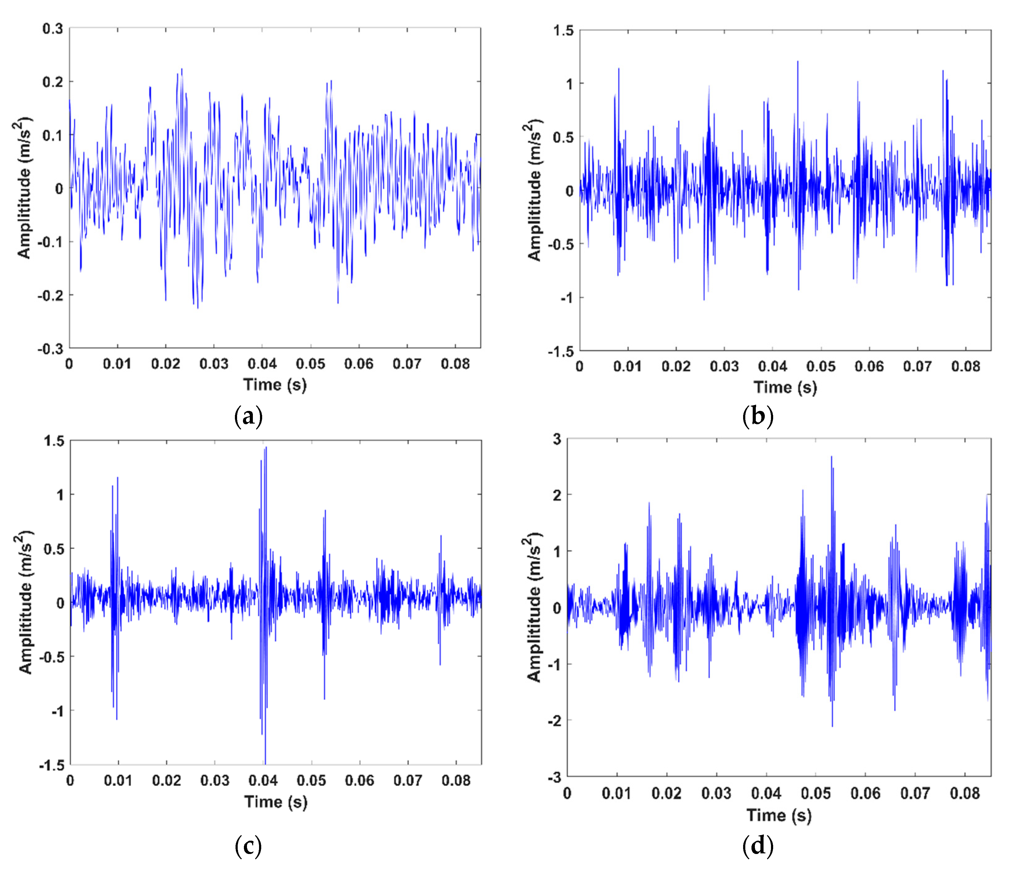
Figure 6 shows the time-domain waveforms of the vibration signals of bearings with different fault severity degrees at the inner race. Comparing Figure 7a with Figure 7b–d, it is obvious that we can easily determine whether a fault occurs or not, as the signal of the inner race with a fault of 0.000 in was a normal signal distinct from fault signals. From Figure 7b–d, we find that all fault signals have prominent impact components with different amplitudes. However, the differences between the signals of different fault severity degrees were insufficient to accurately distinguish the fault severity degrees of the inner race.
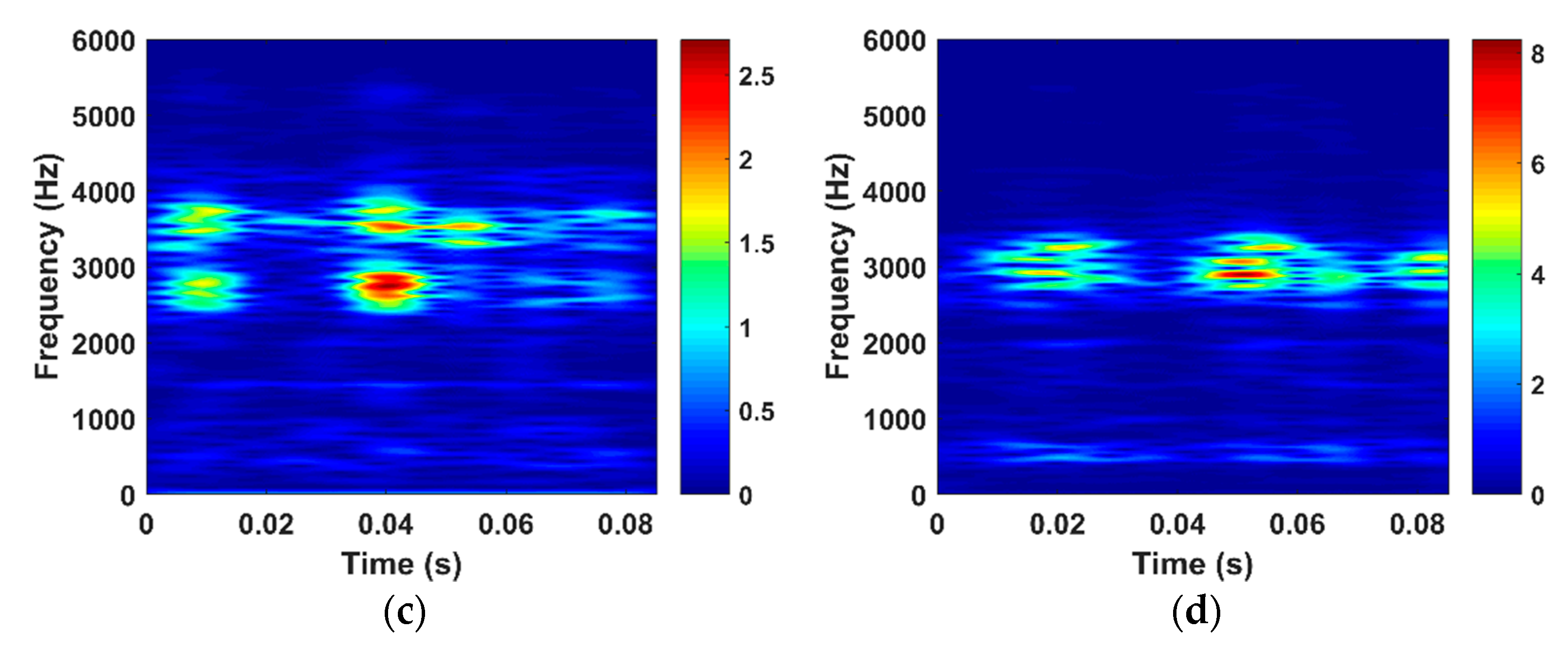
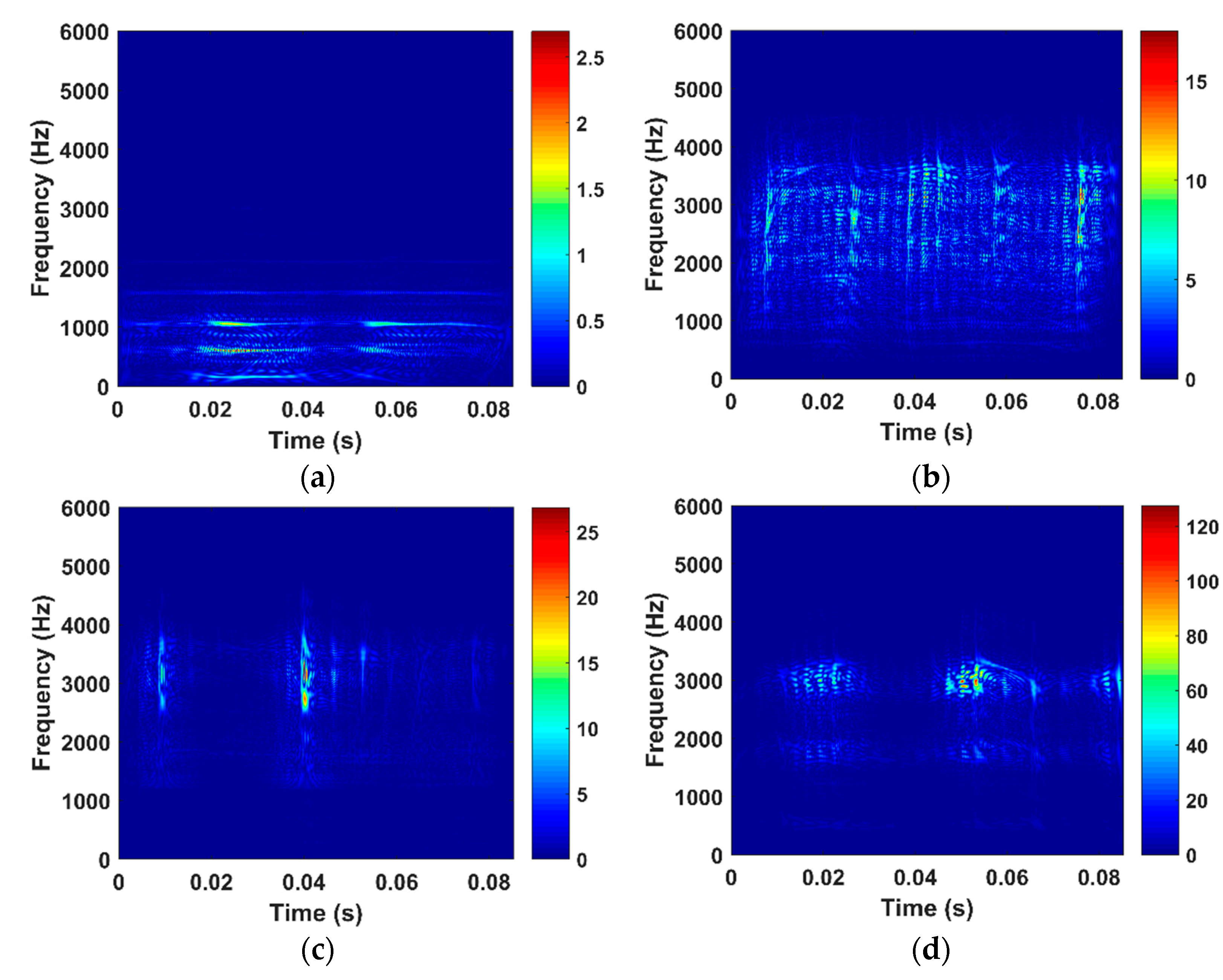
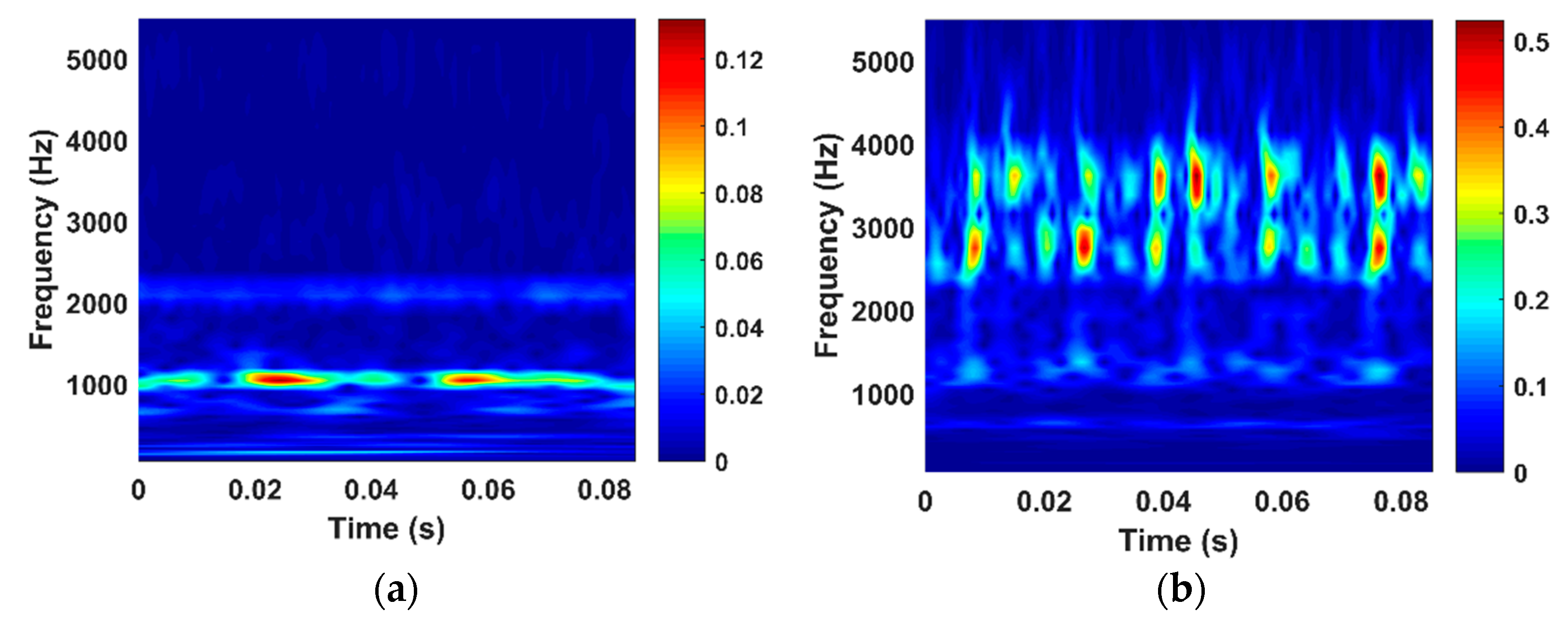
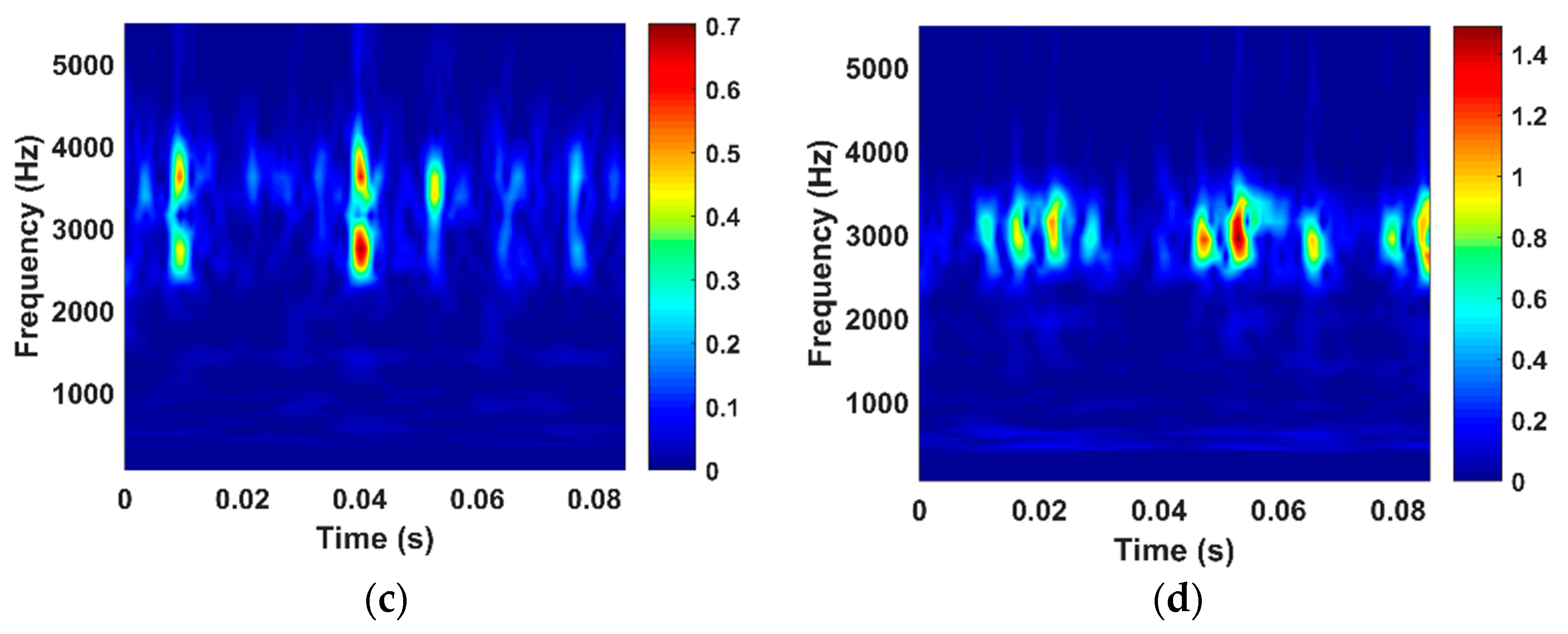
In this study, the STFA-PD method was employed to process the vibration signals. For comparison, the STFT, PWVD, and WT were used to conduct the time–frequency analysis of the signals with different fault severity degrees at the inner race. Figure 8, Figure 9, Figure 10 and Figure 11 show the TFIs obtained using the STFT, PWVD, WT, and STFA-PD, respectively.
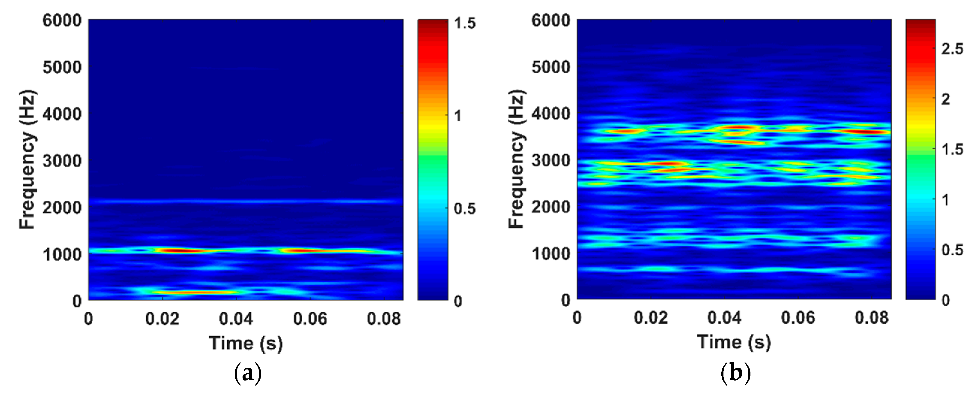
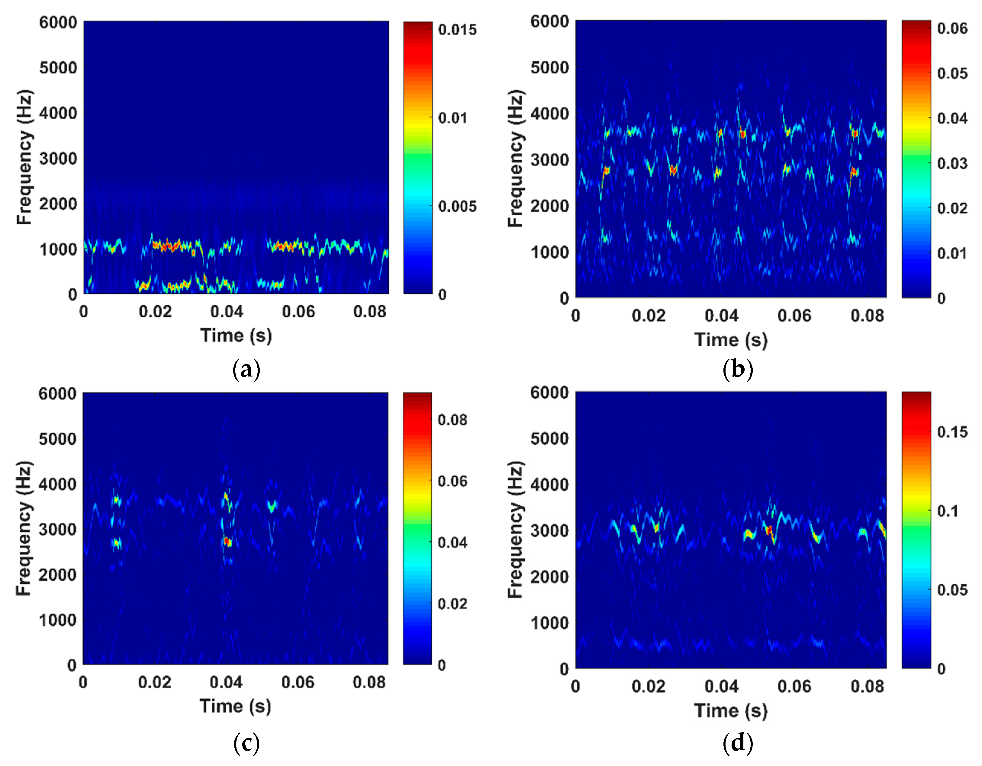
The energy distribution in the frequency domain of the normal signal was found to be narrow and relatively centralized in the low-frequency band. When an inner race fault occurs, the energy distributions became very wide, and the energy was mostly concentrated in the high-frequency band ranging from 2500 Hz to 3500 Hz. All TFIs obtained from the fault signals showed certain proportions of high-frequency impact components corresponding to the time-domain waveforms of the vibration signals. Moreover, the proportion of high-frequency impact components increased with an increase in the fault severity degree.
Figure 8 shows that the time–frequency concentration and resolution of the traditional STFT were low and the TFIs could not accurately express the time–frequency characteristics of the vibration signals. In addition, there were obvious noise interferences in the TFIs. On the contrary, the TFIs obtained using the PWVD were good in terms of the time–frequency concentration and resolution, and the TFIs of different fault severity degrees could be accurately distinguished. However, they suffered from cross-term interferences, and thus, could not precisely reflect the time–frequency characteristics of the vibration signals, as shown in Figure 9. As shown in Figure 10, similar to the STFT method, the TFIs obtained using the WT were not subjected to cross-term interferences. Moreover, we found that the WT had a relatively good distinctiveness. However, the frequency resolution obtained using the WT was lower than that obtained using the STFT, although its time resolution was better. Additionally, as the WT is essentially a type of time-scale transform and there is no good correspondence between scale and frequency, the WT could not accurately express the frequency changes in the signals with respect to time.
Compared to Figure 8, Figure 9 and Figure 10, Figure 11 shows that the time–frequency concentration and resolution of the STFA-PD were higher than the STFT, PWVD, and WT methods, and there was no cross-term interference problem. Moreover, the STFA-PD filtered out a lot of noise, which made the characteristics of the high-frequency impact more obvious. The differences between the TFIs of different fault severity degrees were higher than those obtained using the other three methods. As a result, the STFA-PD can better express the time–frequency characteristics of the signals, and thus, build a good foundation to extract the texture features for an effective characterization of bearings with different fault severity degrees.
4.3. GLCM-Based Texture Features of Sparse Time–Frequency Images
To extract the GLCM-based texture features from sparse TFIs, the colored TFIs shown in Figure 10 should be transformed into gray images. In this study, the weighted average method was used to convert the color images into corresponding gray images, each of which had a pixel size of 429 × 543 and contained 256 gray levels ranging from 0 to 255. Moreover, given the characteristics of the TFIs shown above, the offset values were taken as , , , and corresponding to the four directions , respectively. We then obtained the GLCMs with , and thus, extracted the 12 texture features for each gray image.
As mentioned above, 80 samples were chosen for Test 1. By extracting the GLCM-based texture features from each sample, we obtained values of the 12 features in Test 1, as shown in Figure 12. The samples were numbered from 1 to 80. No. 1 to No. 20 denoted normal (0.000 in) samples, No. 21 to No. 40 denoted samples with a mild fault severity degree (0.007 in) at the inner race, No. 41 to No. 60 denoted samples with a moderate fault severity degree (0.014 in) at the inner race, and No. 61 to No. 80 denoted samples with a severe fault severity degree (0.021 in) at the inner race.
The 12 texture features were found to have a relatively low discreteness for the same fault severity degree and good discrimination capability between different fault severity degrees. Therefore, the features could be used to conduct the classification of fault severity degrees of the bearings. From a discrimination viewpoint, among the 12 features, the energy features (T9, T10, T11, and T12) were the best, followed by the entropy features (T1, T2, T3, and T4). The contrast features (T5, T6, T7, and T8) performed the worst. The distribution range of each contrast feature of the samples was wide, and the distributions of the samples with different fault severity degrees overlapped with each other in various degrees.
In addition, we found that, although a single feature had a certain degree of discrimination, it could not completely separate different fault severity degrees, given the observed overlap of sample distributions with different fault severity degrees. Consequently, it was necessary to employ multiple features for pattern recognition.
4.4. Fault Severity Classification
To realize automatic classification of the GLCM-based texture features and evaluate the performance of the sparse TFI texture feature extraction method proposed in this paper, the 1-nearest neighbor classifier (1NNC) [54] and least squares support vector machine (LS-SVM) [55,56,57] were employed. Both these classifiers are commonly used for pattern recognition, and have stable classification performance and high efficiency. The LS-SVM was performed using LS-SVMlab1.8 [58], and the cross-validation method was used to optimize the parameters. Moreover, the linear kernel function was selected as the kernel function of the LS-SVM.
As mentioned above, 80 samples were chosen for each test. The dataset of each test was divided into two groups: 40 samples (20 samples for each severity degree) were used as the training dataset and the remaining 40 samples as the testing dataset. The process of random grouping, training, and classification was conducted 10 times to obtain more robust results. The average classification accuracy was used as a performance evaluation index for the proposed method.
Table 2 lists the results of the bearing fault severity recognition. The performance of the STFA-PD was the best of the four time–frequency analysis methods, because it had higher time–frequency concentration and resolution than the others, which made the texture features extracted from the sparse TFIs more accurate for representing differences between the samples with different fault severity degrees.
Moreover, the results of the first two tests were better than those of the third one, because the third test was on the ball fault severity recognition. The vibration signals of ball faults were more complex than those of outer race and inner race faults, making the TFIs more complex. Consequently, it was more difficult to use texture features to characterize the signals and obtain better classification accuracy in Test 3 compared with Tests 1 and 2. Nevertheless, the classification accuracy of LS-SVM using the STFA-PD-based texture features was 96.50% in Test 3. The WT-based texture features also yielded satisfactory results; however, they were not always as good as those obtained using the STFA-PD-based features.
5. Conclusions
In this paper, an approach for the bearing fault severity monitoring based on the texture feature extraction of sparse TFIs was proposed. The STFA-PD was developed to obtain the sparse TFIs. Then, the GLCM-based texture features of the sparse TFIs were extracted for an automatic classification to realize fault severity monitoring.
The developed STFA-PD was validated using a simulated signal. The result showed that the STFA-PD method can overcome the drawbacks of the traditional time–frequency analysis methods, such as low resolution and cross-term interference. Moreover, it was found that the STFA-PD method is better in terms of denoising performance. Therefore, the STFA-PD method can be used to obtain high-quality TFIs without suffering from cross-term interference. Since the STFA-PD method is a universal time-frequency analysis method, it can be used to analyze other non-stationary signals.
Experiments were conducted on the popular CWRU bearing dataset to validate the effectiveness of the proposed bearing fault severity monitoring approach. It was found that the STFA-PD method obtained the most high-quality TFIs of bearing vibration signals. As a result, the proposed approach obtained higher overall accuracy than those based on STFT, PWVD, and WT. This study clearly showed that the proposed approach has significant potential to be a powerful tool for the fault severity monitoring of rolling bearings and can be applied to other rotating machinery such as gearboxes and rotors.
However, there were some limitations to the proposed approach. One is that a training feature set is needed for this approach. In practice, this set is often difficult to obtain, which restricts the application of the approach. Future work will focus on monitoring the bearing fault severity without a training feature set. Noting that 1NNC and LS-SVM are supervised learning algorithms, in future work, we will attempt to use some semi-supervised or unsupervised learning algorithms to recognize the bearing fault severity. Another limitation of the proposed approach is that the GLCM-based features are not correlated with physical significance. We cannot identify the bearing fault severity from the feature values. In the future, we intend to search for or construct more powerful features with physical meaning to more effectively capture the pattern of fault severity. The energy (or amplitude) information of signals expressed by the TFIs will be used in future studies to extract features correlated with physical significance.
Author Contributions
All authors discussed and agreed upon the idea and made scientific contributions. Y.D. and Y.C. conceived the original idea and designed the experiments; J.D. and Y.X. conducted the experiments; Y.D. wrote the paper. G.M. is the advisor of Y.D., provided the funding, and revised the paper.
Funding
This research was funded by the National Key Research and Development Program of China (Grant number 2016YFC0600900), the Yue Qi Distinguished Scholar Project of China University of Mining & Technology(Beijing) (Grant number 800015Z1145), the National Natural Science Foundation of China (Grant number U1361127), the Fundamental Research Funds for the Central Universities (Grant number 00/800015HJ), the Education and Scientific Research Foundation of Education Department of Fujian Province for Middle-aged and Young Teachers (Grant number JAT170352), the Foundation of Department of Education of Guangdong Province (Grant number 2017KCXTD015), and the Open Foundation of Digital Signal and Image Processing Key Laboratory of Guangdong Province (Grant number 2017GDDSIPL-01). The APC was funded by the National Natural Science Foundation of China (Grant number U1361127).
Acknowledgments
The authors would like to thank for the supports of all the fundings. The authors would also like to thank Editage [www.editage.cn] for English language editing.
Conflicts of Interest
The authors declare no conflict of interest.
Nomenclature
| TFIs | time–frequency image |
| SR | sparse representation |
| GLCM | gray level co-occurrence matrix |
| STFA-PD | sparse time–frequency analysis method based on the first-order primal-dual algorithm |
| FFT | fast Fourier transform |
| STFT | short-time Fourier transform |
| ST | S transform |
| WVD | Wigner–Ville distribution |
| PWVD | pseudo Wigner–Ville distribution |
| WT | wavelet transform |
| TFR | time–frequency representation |
| TD-2DPCA | two-direction two-dimensional principal component analysis |
| TD-2DLDA | two-direction two-dimensional linear discriminant analysis |
| 2DNMF | two-dimensional non-negative matrix factorization |
| FT | Fourier transform |
| IFT | inverse Fourier transform |
| continuous-time signal | |
| continuous-time sliding window function of time index | |
| STFT coefficient of at time index and frequency | |
| discrete signal of period N, where | |
| discrete sliding window function of time index n | |
| discrete STFT coefficient of at time index and frequency | |
| period of discrete signal | |
| operator of Fourier transform coefficient | |
| Fourier transform coefficient | |
| inverse Fourier transform matrix ; where | |
| windowed signal at time , | |
| Fourier spectrum of , | |
| short-time truncated sub-signal at time index | |
| sliding window matrix at time , | |
| sliding window matrix at time , | |
| estimated signal spectrum at time | |
| sparse time–frequency spectrum, | |
| user-specified parameter related to the noise | |
| sparse coefficient, | |
| convex set, | |
| dual variable, | |
| sparse term of Equation (9) | |
| convex conjugate function of , | |
| fidelity term of Equation (9) | |
| leaning ratios, | |
| acceleration factor, | |
| the maximum number of iterations | |
| value of in the th iteration | |
| value of in the th iteration | |
| value of in the th iteration | |
| value of in the th iteration | |
| acceleration variable of in the th iteration | |
| acceleration variable of in the th iteration | |
| a sinusoidal signal, | |
| a nonlinear frequency-modulated signal, | |
| a nonlinear frequency-modulated signal, | |
| a multi-component simulated signal, | |
| a noisy signal | |
| co-occurrence frequency of a pixel pairs | |
| total number satisfying the conditions | |
| co-occurrence probability |
References
- Cui, L.; Chunqing, M.A.; Zhang, F.; Wang, H. Quantitative diagnosis of fault severity trend of rolling element bearings. Chin. J. Mech. Eng. 2015, 28, 1254–1260. [Google Scholar] [CrossRef]
- Glowacz, A.; Glowacz, W.; Glowacz, Z.; Kozik, J. Early fault diagnosis of bearing and stator faults of the single-phase induction motor using acoustic signals. Measurement 2018, 113, 1–9. [Google Scholar] [CrossRef]
- Berredjem, T.; Benidir, M. Bearing faults diagnosis using fuzzy expert system relying on an improved range overlaps and similarity method. Expert Syst. Appl. 2018, 108, 134–142. [Google Scholar] [CrossRef]
- Hong, H.; Liang, M. Fault severity assessment for rolling element bearings using the Lempel–Ziv complexity and continuous wavelet transform. J. Sound Vib. 2009, 320, 452–468. [Google Scholar] [CrossRef]
- Hong, S.; Zhou, Z.; Zio, E.; Hong, K. Condition assessment for the performance degradation of bearing based on a combinatorial feature extraction method. Dig. Signal Process. 2014, 27, 159–166. [Google Scholar] [CrossRef]
- Duan, Z.; Wu, T.; Guo, S.; Shao, T.; Malekian, R.; Li, Z. Development and trend of condition monitoring and fault diagnosis of multi-sensors information fusion for rolling bearings: A review. Int. J. Adv. Manuf. Technol. 2018, 96, 803–819. [Google Scholar] [CrossRef]
- Wang, H.; Chen, J. Performance degradation assessment of rolling bearing based on bispectrum and support vector data description. J. Vib. Control 2013, 20, 2032–2041. [Google Scholar] [CrossRef]
- Cerrada, M.; Sánchez, R.; Li, C.; Pacheco, F.; Cabrera, D.; José, V.D.O.; Vásquez, R.E. A review on data-driven fault severity assessment in rolling bearings. Mech. Syst. Signal Process. 2018, 99, 169–196. [Google Scholar] [CrossRef]
- Molina, M.A.; Gohar, R. Hydrodynamic lubrication of ball-bearing cage pockets. ARCHIVE J. Mech. Eng. Sci. 1978, 20, 11–20. [Google Scholar] [CrossRef]
- Rahnejat, H.; Gohar, R. The vibrations of radial ball bearings. ARCHIVE Proc. Inst. Mech. Eng. C J. Mech. Eng. Sci. 1985, 199, 181–193. [Google Scholar] [CrossRef]
- Wardle, F.P. Vibration forces produced by waviness of the rolling surfaces of thrust loaded ball bearings, part 1: Theory. Proc. Inst. Mech. Eng. 1988, 202, 305–312. [Google Scholar] [CrossRef]
- Johns-Rahnejat, P.; Gohar, R. Point contact elastohydrodynamic pressure distribution and sub-surface stress field. In Proceedings of the International Tri-Annual Conference on Multi-Body Dynamics: Monitoring and Simulation Techniques, Bradford, UK, 25–27 March 1997; pp. 161–177. [Google Scholar]
- Rai, A.; Upadhyay, S.H. A review on signal processing techniques utilized in the fault diagnosis of rolling element bearings. Tribol. Int. 2016, 96, 289–306. [Google Scholar] [CrossRef]
- Borghesani, P.; Ricci, R.; Chatterton, S.; Pennacchi, P. A new procedure for using envelope analysis for rolling element bearing diagnostics in variable operating conditions. Mech. Syst. Signal Process. 2013, 38, 23–35. [Google Scholar] [CrossRef]
- Randall, R.B.; Antoni, J. Rolling element bearing diagnostics—A tutorial. Mech. Syst. Signal Process. 2011, 25, 485–520. [Google Scholar] [CrossRef]
- Peeters, C.; Guillaume, P.; Helsen, J. A comparison of cepstral editing methods as signal pre-processing techniques for vibration-based bearing fault detection. Mech. Syst. Signal Process. 2017, 91, 354–381. [Google Scholar] [CrossRef]
- Bi, G.; Chen, J.; He, J.; Zhou, F.; Zhang, G.C. Application of degree of cyclostationarity in rolling element bearing diagnosis. Key Eng. Mater. 2005, 293–294, 347–354. [Google Scholar] [CrossRef]
- Liu, X.; Bo, L.; Peng, C. Application of order cyclostationary demodulation to damage detection in a direct-driven wind turbine bearing. Meas. Sci. Technol. 2014, 25, 25004–25011. [Google Scholar] [CrossRef]
- Acuña, D.Q.; Vicuña, C.M. Damage Assessment of Rolling Element Bearing Using Cyclostationary Processing of Ae Signals with Electromagnetic Interference; Springer International Publishing: Basel, Switzerland, 2015; pp. 43–54. [Google Scholar]
- Feng, Z.; Liang, M.; Chu, F. Recent advances in time–frequency analysis methods for machinery fault diagnosis: A review with application examples. Mech. Syst. Signal Process. 2013, 38, 165–205. [Google Scholar] [CrossRef]
- Zhao, M.; Tang, B.; Tan, Q. Fault diagnosis of rolling element bearing based on s transform and gray level co-occurrence matrix. Meas. Sci. Technol. 2015, 26, 085008. [Google Scholar] [CrossRef]
- Peng, Z.K.; Chu, F.L. Application of the wavelet transform in machine condition monitoring and fault diagnostics: A review with bibliography. Mech. Syst. Signal Process. 2004, 18, 199–221. [Google Scholar] [CrossRef]
- Chen, Y.P.; Peng, Z.M.; He, Z.H.; Lin, T.; Zhang, D.J. The optimal fractional gabor transform based on the adaptive window function and its application. Appl. Geophys. 2013, 10, 305–313. [Google Scholar] [CrossRef]
- Chen, Y.; Peng, Z.; Cheng, Z.; Tian, L. Seismic signal time-frequency analysis based on multi-directional window using greedy strategy. J. Appl. Geophys. 2017, 143, 116–128. [Google Scholar] [CrossRef]
- Cohen, L. Time-frequency distribution—A review. Proc. IEEE 1989, 77, 941–981. [Google Scholar] [CrossRef]
- Hlawatsch, F.; Boudreaux-Bartels, G.F. Linear and quadratic time-frequency signal representations. IEEE Signal Process. Mag. 1992, 9, 21–67. [Google Scholar] [CrossRef]
- Hess-Nielsen, N.; Wickerhauser, M.V. Wavelets and time-frequency analysis. Proc. IEEE 1996, 84, 523–540. [Google Scholar] [CrossRef] [Green Version]
- Sejdić, E.; Djurović, I.; Jiang, J. Time–frequency feature representation using energy concentration: An overview of recent advances. Digit. Signal Process. 2009, 19, 153–183. [Google Scholar] [CrossRef]
- Stockwell, R.G.; Mansinha, L.; Lowe, R.P. Localization of the complex spectrum: The s transform. IEEE Trans. Signal Process. 1996, 44, 998–1001. [Google Scholar] [CrossRef]
- Vafaei, S.; Rahnejat, H. Indicated repeatable runout with wavelet decomposition (irr-wd) for effective determination of bearing-induced vibration. J. Sound Vib. 2003, 260, 67–82. [Google Scholar] [CrossRef]
- Mallat, S.G.; Zhang, Z. Matching pursuits with time-frequency dictionaries. IEEE Trans. Signal Process. 1993, 41, 3397–3415. [Google Scholar] [CrossRef] [Green Version]
- Chen, S.S.; Donoho, D.L.; Saunders, M.A. Atomic decomposition by basis pursuit. Siam Rev. 2001, 43, 129–159. [Google Scholar] [CrossRef]
- Borgnat, P.; Flandrin, P. Time-frequency localization from sparsity constraints. In Proceedings of the IEEE International Conference on Acoustics, Speech and Signal Processing, Las Vegas, NV, USA, 31 March 2008–4 April 2008; pp. 3785–3788. [Google Scholar]
- Elad, M. Sparse and Redundant Representations: From Theory to Applications in Signal and Image Processing; Springer Publishing Company, Incorporated: Basel, Switzerland, 2010; pp. 1094–1097. [Google Scholar]
- Cheng, H.; Liu, Z.; Yang, L.; Chen, X. Sparse representation and learning in visual recognition: Theory and applications. Signal Process. 2013, 93, 1408–1425. [Google Scholar] [CrossRef]
- Wang, C.; Gan, M.; Zhu, C.A. Fault feature extraction of rolling element bearings based on wavelet packet transform and sparse representation theory. J. Intell. Manuf. 2015, 11, 1–15. [Google Scholar] [CrossRef]
- Liu, Z.; Wei, X.; Li, X. Aliasing-free micro-doppler analysis based on short-time compressed sensing. Signal Process. IET 2013, 8, 176–187. [Google Scholar] [CrossRef]
- Liu, Z.; You, P.; Wei, X.; Liao, D.; Li, X. High resolution time-frequency distribution based on short-time sparse representation. Circ. Syst. Signal Process. 2014, 33, 3949–3965. [Google Scholar] [CrossRef]
- Gholami, A. Sparse time–frequency decomposition and some applications. IEEE Trans. Geosci. Remote Sens. 2013, 51, 3598–3604. [Google Scholar] [CrossRef]
- Hu, J.; He, X.; Li, W.; Ai, H.; Li, H.; Xie, J. Parameter estimation of maneuvering targets in othr based on sparse time-frequency representation. J. Syst. Eng. Electron. 2016, 27, 574–580. [Google Scholar] [CrossRef]
- Chambolle, A.; Pock, T. A first-order primal-dual algorithm for convex problems with applications to imaging. J. Math. Imaging Vis. 2011, 40, 120–145. [Google Scholar] [CrossRef]
- Sidky, E.Y.; Jørgensen, J.H.; Pan, X. Convex optimization problem prototyping for image reconstruction in computed tomography with the chambolle-pock algorithm. Phys. Med. Biol. 2012, 57, 3065–3091. [Google Scholar] [CrossRef] [PubMed]
- Li, B.; Zhang, P.L.; Liu, D.S.; Mi, S.S.; Ren, G.Q.; Tian, H. Feature extraction for rolling element bearing fault diagnosis utilizing generalized s transform and two-dimensional non-negative matrix factorization. J. Sound Vib. 2011, 330, 2388–2399. [Google Scholar] [CrossRef]
- Wang, W.G.; Liu, Z.S. Classification of time-frequency images based on locality-constrained linear coding optimization model for rotating machinery fault diagnosis. ARCHIVE Proc. Inst. Mech. Eng. C J. Mech. Eng. Sci. 2015, 229, 3350–3360. [Google Scholar] [CrossRef]
- Li, W.; Lin, L.; Shan, W. Bearing fault diagnosis based on generalized s-transform and two-directional 2dpca. Zhendong Ceshi Yu Zhenduan/J. Vib. Meas. Diagn. 2015, 35, 499–506. [Google Scholar]
- Li, B.; Zhang, P.L.; Liu, D.S.; Mi, S.S.; Liu, P.Y. Classification of time-frequency representations based on two-direction 2dlda for gear fault diagnosis. Appl. Soft Comput. J. 2011, 11, 5299–5305. [Google Scholar] [CrossRef]
- Haraclick, R.M. Texture features for image classification. IEEE Trans. Syst. Man. Cybern. 1973, 3, 610–621. [Google Scholar] [CrossRef]
- Nawab, S.H. Short-Time Fourier Transform. Adv. Top. Signal Process. 1988, 32, 289–337. [Google Scholar]
- Pantic, I.; Dimitrijevic, D.; Nesic, D.; Petrovic, D. Gray level co-occurrence matrix algorithm as pattern recognition biosensor for oxidopamine-induced changes in lymphocyte chromatin architecture. J. Theor. Biol. 2016, 406, 124–128. [Google Scholar] [CrossRef] [PubMed]
- Baraldi, A.; Parmiggiani, F. Investigation of the textural characteristics associated with gray level cooccurrence matrix statistical parameters. IEEE Trans. Geosci. Remote Sens. 1995, 33, 293–304. [Google Scholar] [CrossRef]
- Smith, W.A.; Randall, R.B. Rolling element bearing diagnostics using the case western reserve university data: A benchmark study. Mech. Syst. Signal Process. 2015, 64–65, 100–131. [Google Scholar] [CrossRef]
- Loparo, K.A. Bearings Vibration Data Set, Case Western Reserve University. Available online: http://csegroups.case.edu/bearingdatacenter/pages/download-data-file (accessed on 27 October 2017).
- Pang, B.; Tang, G.; Tian, T.; Zhou, C. Rolling bearing fault diagnosis based on an improved htt transform. Sensors 2018, 18, 1203. [Google Scholar] [CrossRef] [PubMed]
- Grother, P.J.; Candela, G.T.; Blue, J.L. Fast implementations of nearest neighbor classifiers. Pattern Recognit. 1997, 30, 459–465. [Google Scholar] [CrossRef] [Green Version]
- Ye, J.; Xiong, T. Svm versus least squares svm. J. Mach. Learn. Res. 2007, 2, 644–651. [Google Scholar]
- Zhang, Y.; Zhang, C.; Sun, J.; Jingjing, G. Improved wind speed prediction using empirical mode decomposition. Adv. Electr. Comput. Eng. 2018, 18, 3–10. [Google Scholar] [CrossRef]
- Zhang, C.; Peng, Z.; Chen, S.; Li, Z.; Wang, J. A gearbox fault diagnosis method based on frequency-modulated empirical mode decomposition and support vector machine. ARCHIVE Proc. Inst. Mech. Eng. C J. Mech. Eng. Sci. 2016, 232, 369–380. [Google Scholar] [CrossRef]
- Ls-svmlab1.8. Available online: http://www.esat.kuleuven.ac.be/sista/lssvmlab/ (accessed on 14 January 2018).
Figure 1.
Flowchart of the proposed approach.

Figure 2.
(a) Time-domain waveform of the simulated signal and its time–frequency images (TFIs) obtained using (b) short-time Fourier transform (STFT), (c) pseudo Wigner–Ville distribution (PWVD), (d) wavelet transform (WT), and (e) the sparse time–frequency analysis method based on the first-order primal-dual algorithm (STFA-PD).

Figure 3.
(a) Time-domain waveform of the noisy signal with the signal-to-noise ratio (SNR) of −2 dB, and its TFIs obtained using (b) STFT, (c) PWVD, (d) WT, and (e) STFA-PD.
Figure 3.
(a) Time-domain waveform of the noisy signal with the signal-to-noise ratio (SNR) of −2 dB, and its TFIs obtained using (b) STFT, (c) PWVD, (d) WT, and (e) STFA-PD.

Figure 4.
Peak SNR (PSNR) values obtained by different methods (i.e., STFT, PWVD, WT, and the proposed STFA-PD method) at different SNR levels.
Figure 4.
Peak SNR (PSNR) values obtained by different methods (i.e., STFT, PWVD, WT, and the proposed STFA-PD method) at different SNR levels.

Figure 5.
Calculation schematic of gray level co-occurrence matrix (GLCM).

Figure 6.
(a) Bearing test stand, and (b) its structural diagram.

Figure 7.
Time-domain waveforms of the vibration signals of bearings with four different faults severity degrees at the inner race: (a) 0.000 in, (b) 0.007 in, (c) 0.014 in, and (d) 0.021 in.
Figure 7.
Time-domain waveforms of the vibration signals of bearings with four different faults severity degrees at the inner race: (a) 0.000 in, (b) 0.007 in, (c) 0.014 in, and (d) 0.021 in.

Figure 8.
TFIs obtained using the STFT from bearing vibration signals of different severity degrees: (a) 0.000 in, (b) 0.007 in, (c) 0.014 in, and (d) 0.021 in.
Figure 8.
TFIs obtained using the STFT from bearing vibration signals of different severity degrees: (a) 0.000 in, (b) 0.007 in, (c) 0.014 in, and (d) 0.021 in.


Figure 9.
TFIs obtained using the PWVD from bearing vibration signals of different severity degrees: (a) 0.000 in, (b) 0.007 in, (c) 0.014 in, and (d) 0.021 in.
Figure 9.
TFIs obtained using the PWVD from bearing vibration signals of different severity degrees: (a) 0.000 in, (b) 0.007 in, (c) 0.014 in, and (d) 0.021 in.

Figure 10.
TFIs obtained using the WT from bearing vibration signals of different severity degrees: (a) 0.000 in, (b) 0.007 in, (c) 0.014 in, and (d) 0.021 in.
Figure 10.
TFIs obtained using the WT from bearing vibration signals of different severity degrees: (a) 0.000 in, (b) 0.007 in, (c) 0.014 in, and (d) 0.021 in.


Figure 11.
TFIs obtained using the STFA-PD from bearing vibration signals of different severity degrees: (a) 0.000 in, (b) 0.007 in, (c) 0.014 in, and (d) 0.021 in.
Figure 11.
TFIs obtained using the STFA-PD from bearing vibration signals of different severity degrees: (a) 0.000 in, (b) 0.007 in, (c) 0.014 in, and (d) 0.021 in.

Figure 12.
Values of 12 features of samples in Test 1.


Table 1.
Test arrangement of the bearing fault severity.
| Test | Fault Type | Severity Degree (inches) |
|---|---|---|
| 1 | Inner race fault | 0.000 |
| 0.007 | ||
| 0.014 | ||
| 0.021 | ||
| 2 | Outer race fault | 0.000 |
| 0.007 | ||
| 0.014 | ||
| 0.021 | ||
| 3 | Ball fault | 0.000 |
| 0.007 | ||
| 0.014 | ||
| 0.021 |
Table 2.
Results of bearing fault severity recognition.
| Method | Accuracy (%) | |||
|---|---|---|---|---|
| Test 1 | Test 2 | Test 3 | ||
| STFA-PD | 1NNC | 99.50 | 99.25 | 83.75 |
| STFT | 97.00 | 97.00 | 77.25 | |
| PWVD | 85.75 | 94.00 | 75.00 | |
| WT | 91.50 | 98.75 | 74.00 | |
| STFA-PD | LS-SVM | 100.00 | 100.00 | 96.50 |
| STFT | 100.00 | 100.00 | 84.25 | |
| PWVD | 98.25 | 99.00 | 84.50 | |
| WT | 100.00 | 100.00 | 93.75 | |
© 2018 by the authors. Licensee MDPI, Basel, Switzerland. This article is an open access article distributed under the terms and conditions of the Creative Commons Attribution (CC BY) license (http://creativecommons.org/licenses/by/4.0/).
Share and Cite
MDPI and ACS Style
Du, Y.; Chen, Y.; Meng, G.; Ding, J.; Xiao, Y. Fault Severity Monitoring of Rolling Bearings Based on Texture Feature Extraction of Sparse Time–Frequency Images. Appl. Sci. 2018, 8, 1538. https://doi.org/10.3390/app8091538
AMA Style
Du Y, Chen Y, Meng G, Ding J, Xiao Y. Fault Severity Monitoring of Rolling Bearings Based on Texture Feature Extraction of Sparse Time–Frequency Images. Applied Sciences. 2018; 8(9):1538. https://doi.org/10.3390/app8091538
Chicago/Turabian StyleDu, Yan, Yingpin Chen, Guoying Meng, Jun Ding, and Yajing Xiao. 2018. "Fault Severity Monitoring of Rolling Bearings Based on Texture Feature Extraction of Sparse Time–Frequency Images" Applied Sciences 8, no. 9: 1538. https://doi.org/10.3390/app8091538
Note that from the first issue of 2016, this journal uses article numbers instead of page numbers. See further details here.