Study on EEMD-Based KICA and Its Application in Fault-Feature Extraction of Rotating Machinery

Featured application

This work can extract fault features of single-channel vibration signals of rotating machinery.

Abstract

A method is proposed to improve the feature extraction of vibration signals of rotating machinery. Firstly, the single-channel vibration signal is decomposed with ensemble empirical mode decomposition (EEMD). Then, the number of fault signals can be estimated with singular-value decomposition (SVD). Finally, the fault signals can be extracted with kernel-independent component analysis (KICA). The advantage of this method is that it can estimate the number of fault signals of single-channel vibration signals and can extract the fault features clearly. Compared with wavelets, empirical mode decomposition (EMD), variational mode decomposition (VMD) and EEMD, the better performance of this method is proven with three experimental analyses of faulty gear, a faulty rolling bearing and a faulty shaft. The results demonstrate that the proposed method is efficient to extract the fault features of single-channel vibration signals of rotating machinery.

1. Introduction

The faults of gears, rolling bearings and shafts of rotating machinery are disastrous for the whole machinery. Many studies on fault diagnosis of rotating machinery have been published [1,2,3]. However, due to cost issues and limited monitoring environments, multiple sensors cannot be installed on rotating machinery, and sometimes it is even single-channel monitoring. In order to acquire more fault information of single-channel vibration signals of rotating machinery and improve the efficiency of fault diagnosis, many feature extraction methods have been proposed, such as wavelets [4,5], empirical mode decomposition (EMD) [6,7], ensemble empirical mode decomposition (EEMD) [8,9], variational mode decomposition (VMD) [10,11] and so on. However, these methods have the problem that the extracted features sometimes are not clear enough, they cannot estimate the number of fault signals, and they need to be searched artificially from all component signals. In recent years, blind source separation (BSS) has been applied more and more to diagnose the faults of rotating machinery [12,13]. The goal of BSS is to estimate latent signals from the mixed signals without any knowledge of the mixing process. Kernel-independent component analysis (KICA) is one of the most famous algorithms of BSS [14,15]. The vibration signal of large rotating machinery often mixes several signals and shows a strong nonlinear characteristic. The advantage of KICA is that both linear signals and nonlinear signals can be separated.

Estimating the number of latent signals accurately is an important prerequisite for an effective separation of a blind signal. The typical methods are spatial smoothing rank (SSR) [16,17] and information theory [18,19], but they all have some limitations, such as signal-to-noise ratio (SNR). Singular-value decomposition (SVD) is a nonparametric technique [20,21]. Listing the singular values in descending order first, the sequence number of the maximum ratio of neighboring singular values (NSVR) can be applied to estimate the number of source signals, and it has a good estimation effect under a large number of coherent signals, as well as low SNR.

In this paper, a fault-feature extraction method of single-channel vibration signals based on EEMD-based KICA is proposed, and the number of fault signals is estimated by SVD. The three experimental analyses show that this method has a better performance than wavelets, EMD, VMD and EEMD to extract the fault features of rotating machinery. Its advantage is that the number of fault signals of a single-channel vibration signal can be estimated and the extracted fault features are obvious. This method only needs to input a single-channel vibration signal, and the outputs are fault signals and number, without artificial selection, which improves the efficiency of fault-feature extraction.

The structure of this paper is as follows: The theory of EEMD, correlation coefficients, SVD and KICA are introduced in Section 2. The mathematical model of the proposed method is in Section 3. The performance of the proposed method with faulty gear is evaluated by an experimental analysis in Section 4.1, and the performance of the proposed method with a faulty rolling bearing is evaluated in Section 4.2. In Section 4.3, a faulty shaft experiment proves the effectiveness of the proposed method. The conclusion of this paper is presented in Section 5.

2. Theory

2.1. EEMD

Huang et al. [22] reported that any signal is made up of several intrinsic mode functions (IMFs). The instantaneous frequency of any point of each IMF is meaningful. A signal is formed by the superposition of many IMFs. Huang proposed the EEMD algorithm in 2009, that is, the white Gaussian noise is introduced in the decomposition process. Although white Gaussian noise is added to each IMF, as the noise added at each time of decomposition is random, it can be eliminated by the decomposition of enough times and the ensemble averaging. The procedure of EEMD is as follows:

Step 1: White Gaussian noise with the mean value of zero and constant amplitude standard deviation is added to the decomposed signal $x(t)$, and the signal after adding noise is normalized.

Step 2: EMD is used to decompose the normalized signal to obtain each IMF.

Step 3: Step 1 and Step 2 are repeated n times, ensuring the noise added at every time obeys a normal distribution.

Step 4: Ensemble averaging of the n sets of IMFs obtained from EMD. According to the rule in statistics, the statistical mean of an uncorrelated random sequence is zero, and the influence of white Gaussian noise added to IMFs is removed. Finally, the decomposition of $x(t)$ can be obtained by EEMD, that is,

$$x(t)={\displaystyle \sum _{i=1}^n{\displaystyle \sum _{j=1}^n{c}_{ij}(t)}+{\displaystyle \sum _{j=1}^n{r}_j(t)}},$$

(1)

where $c_i(t)$ is the i-th IMF, and $r(t)$ is redundancy.

The size of the white Gaussian noise added in the iterative process of EMD can directly affect the result of EEMD. The purpose of adding noise in EEMD is to avoid modal aliasing. However, if the noise is too large, it will affect the distribution characteristics of the extreme point intervals of effective high-frequency components. When the noise is too small, it will affect the selection of low-frequency extreme points of signal and lose the function of scale supplement. The criterion for adding white noise to EEMD is as follows:

$$\delta =\frac{{\eta }_h}{{\eta }_f};\beta =\frac{{\eta }_g}{{\eta }_f};0<\beta <\frac{\delta }{2},$$

(2)

where ${\eta }_h$ is the amplitude standard deviation of effective high-frequency component of $x(t)$, ${\eta }_g$ is the amplitude standard deviation of the added white Gaussian noise, and ${\eta }_f$ is the amplitude standard deviation of $x(t)$. Under normal circumstances, when $\beta =\delta /4$, the modal aliasing problem can be effectively avoided. When ${\eta }_g=0.4$ and the number of the ensemble average is 100, a better processing result can be obtained.

EEMD can not only effectively avoid modal aliasing, reduce signal noise and get more meaningful IMFs, it can also decompose a one-dimensional observation signal into a multi-dimensional one, and create a condition for blind source separation.

2.2. Correlation Coefficient

The formula for the correlation coefficient ${\rho }_{x{z}_i}$ of the IMF to the source signal is as follows:

$${\rho }_{x{z}_i}=\frac{\mathrm{cov}(\mathit{X},{\mathit{Z}}_i)}{\sqrt{D(\mathit{X})}\sqrt{D({\mathit{Z}}_i)}},$$

(3)

where $\mathit{X}$ is the mixed source signal, ${\mathit{Z}}_i$ is the i-th IMF, $D(\mathit{X})$ and $D({\mathit{Z}}_i)$ are the variances of signal $\mathit{X}$ and ${\mathit{Z}}_i$, respectively, and $\mathrm{cov}(\mathit{X},{\mathit{Z}}_i)$ is the covariance between the signals $\mathit{X}$ and ${\mathit{Z}}_i$.

2.3. SVD

The signal $\mathit{S}(t)={[s_1(t),\dots ,s_n(t)]}^T$ is contained with n source signals. The observed signal $\mathit{X}(t)={[x_1(t),\dots ,x_m(t)]}^T$ is obtained by m different sensors. The observed signal is assumed to be a linear superposition of source signals and noise signal $\mathit{N}(t)={[n_1(t),\dots ,n_m(t)]}^T$ via a hybrid matrix $\mathit{A}={(a_{ij})}_{m\times n}$. The observed signal $\mathit{X}(t)$ can be described as follows:

$$x_i(t)={\displaystyle \sum _{j=1}^n{a}_{ij}{s}_j(t)}+n_i(t),i=1,2,\cdots ,m,j=1,2,\cdots ,n,$$

(4)

$$\mathit{X}(t)=\mathit{A}\mathit{S}(t)+\mathit{N}(t).$$

(5)

The matrix ${\mathit{R}}_X$ is the covariance matrix of the observed signal $\mathit{X}(t)$, and the eigenvalue decomposition of ${\mathit{R}}_X$ is performed as follows:

$${\mathit{R}}_X=\mathit{Q}\mathit{\Lambda }{\mathit{Q}}^H,$$

(6)

where $\mathit{\Lambda }$ is a diagonal matrix composed of the eigenvalues $\{{\lambda }_1,{\lambda }_2,\dots ,{\lambda }_m\}$ of ${\mathit{R}}_X$. Every column vector of eigenvector $\mathit{Q}$ is a unit eigenvector corresponding to the eigenvalue, and the unit vectors are orthogonal to each other. It can be deduced that the eigenvalues of ${\mathit{R}}_X{\mathit{R}}_X^H$ derived by characteristic decomposition are $\{{\lambda }_1^2,{\lambda }_2^2,\dots ,{\lambda }_m^2\}$. That is,

$${\mathit{R}}_X{\mathit{R}}_X^H=\mathit{Q}\mathit{\Lambda }{\mathit{Q}}^H{(\mathit{Q}\mathit{\Lambda }{\mathit{Q}}^H)}^H=\mathit{Q}{\mathit{\Lambda }}^2{\mathit{Q}}^H.$$

(7)

Therefore, the singular value of ${\mathit{R}}_X$ defined by the singular value is $\left\{\right|{\lambda }_1|,|{\lambda }_2|,\dots ,|{\lambda }_m\left|\right\}$, because the covariance matrix’s singular values are the same as the absolute value of the eigenvalues. So, the number of nonzero eigenvalues is equal to the number of nonzero singular values. It is assumed that ${\tilde{\mathit{R}}}_X$ is the covariance matrix of mixed signal-contained noise. According to the mixed system model $\mathit{X}=\mathit{A}\mathit{S}+\mathit{N}$, the following can be calculated:

$$\begin{array}{ll}{\tilde{\mathit{R}}}_X& =\frac{\mathit{X}{\mathit{X}}^H,}{L}=\frac{(\mathit{A}\mathit{S}+\mathit{{\rm N}}){(\mathit{A}\mathit{S}+\mathit{N})}^H}{L}\\ & =\frac{\mathit{A}\mathit{S}{\mathit{S}}^H{\mathit{A}}^H+\mathit{A}\mathit{S}{\mathit{N}}^H+\mathit{N}{\mathit{S}}^H{\mathit{A}}^H+\mathit{N}{\mathit{N}}^H}{L}\\ & ={\mathit{R}}_{\mathrm{X}}+{\mathit{R}}_N+\frac{\mathit{A}(\mathit{S}{\mathit{N}}^H)+(\mathit{N}{\mathit{S}}^H){\mathit{A}}^H}{L}\end{array}$$

(8)

where L is the number of sampling points, ${\mathit{R}}_N\approx {\sigma }^2\mathit{I}$, $\frac{\mathit{S}{\mathit{N}}^H}{L}\approx 0$, $\frac{\mathit{N}{\mathit{S}}^H}{L}\approx 0$, and then,

$${\tilde{\mathit{R}}}_X={\mathit{R}}_X+{\sigma }^2\mathit{I},$$

(9)

where ${\sigma }^2$ is the power of noise.

If ${\lambda }_1\ge {\lambda }_2\ge \cdots \ge {\lambda }_{k+1}={\lambda }_{k+2}=\cdots ={\lambda }_m=0$ is m eigenvalues of ${\mathit{R}}_X$ and ${\mu }_1\ge {\mu }_2\ge \cdots \ge {\mu }_k$ $\ge {\mu }_{k+1}\ge \cdots \ge {\lambda }_m\ge 0$ is m eigenvalues of ${\tilde{\mathit{R}}}_X$,${\mu }_1\approx {\lambda }_1+{\sigma }^2,{\mu }_2\approx {\lambda }_2+{\sigma }^2,\dots ,{\mu }_k\approx {\lambda }_k+{\sigma }^2,\dots ,{\mu }_m\approx {\lambda }_m+{\sigma }^2$. Therefore, in the case of a high signal-to-noise ratio (SNR), the number of main eigenvalues of the covariance matrix is equal to the number of signals.

The eigenvalues of ${\tilde{\mathit{R}}}_X$ are in descending order, that is,${\mu }_1\ge {\mu }_2\ge \dots \ge {\mu }_m\ge 0$. Let${\gamma }_k={\mu }_k/{\mu }_{k+1},k=1,2,\dots ,m-1$; if ${\gamma }_k$ is the maximum ratio of neighboring singular values, the number of signals will be k.

2.4. KICA

The mathematical description of BSS is: $\mathit{X}=\mathit{A}\mathit{S}+\mathit{N}$, where $\mathit{S}=[s_1(t),s_2(t),\cdots ,s_N(t)]$ is a vector of N source signals, $\mathit{X}=[x_1(t),x_2(t),\cdots ,x_M(t)]$ is a vector of M mixed signals, the mixing matrix $\mathit{A}$ is an M × N dimensional matrix, and $\mathit{N}(t)$ is a noise vector. The meaning is that when the mixing matrix and source signals are unknown, we only determine the remove-mixing matrix $\mathit{W}$ based on the observed data, and the output $\stackrel{⌢}{\mathit{S}}=\mathit{W}\mathit{X}$ is the estimation of source signals.

KICA is not a simple nucleation of independent component analysis (ICA), but a new ICA method. The idea of kernel technology is to use nonlinear mapping$\varphi :R^m\to R$, and map the nonlinear variable $y^i\in R^m(i=1,2,\cdots ,N)$ of original input space into a kernel feature space $R$ to linearize it, and then analyse the mapped data in this feature space. Thus, the linear blind source separation in the space $R$ is equivalent to nonlinear blind source separation in the original space. One of the important characteristics of this technology is that a kernel function can be used instead of an inner product between two vectors to realize nonlinear transformation without specific form being considered. The kernel function of the radial basis function (RBF) $K(x_i,y_i)=\exp (-\parallel x_i-y_i\parallel /{\delta }^2)$ is chosen here.

The characteristic of KICA is to use a nonlinear function in reproducing kernel Hilbert space (RKHS) as a contrast function; the signal is mapped from low-dimensional space to the high-dimensional space, and the kernel method is used to search the minimum value of contrast function in this space. This function has a certain correlation with mutual information and has better mathematical properties. Moreover, this function space is suitable for various source signals. Therefore, compared with traditional ICA, KICA has better flexibility and robustness.

The KICA’s contrast function is constructed by measuring the correlation of a set of random variables directly. Let $F$ be a real vector function space, for simplicity, $s_1$ and $s_2$ are two unary random variables of space $F$. Define the correlation coefficient ${\rho }_F$ of $s_1$ and $s_2$ as the maximum correlation coefficient between random variables $f_1(s_1)$ and $f_2(s_2)$,

$${\rho }_F=\underset{f_1,f_2\in F}{\max }corr(f_1(s_1),f_2(s_2))=\underset{f_1,f_2\in F}{\max }\frac{\mathrm{cov}(f_1(s_1),f_2(s_2))}{{(\mathrm{var}{f}_1(s_1))}^{1/2}{(\mathrm{var}{f}_2(s_2))}^{1/2}}.$$

(10)

${\rho }_F$ is also called a contrast function between random variables. Obviously, if $s_1$ and $s_2$ are independent, then ${\rho }_F=0$. If space $F$ is large enough and ${\rho }_F=0$, then $s_1$ and $s_2$ are also independent of each other. The procedure of KICA is as follows:

Input: data vector $x_1,x_2,\cdots ,x_n$ and kernel function $k(x,s)$.

Step 1: Whiten data vector $x_1,x_2,\cdots ,x_n$.

Step 2: Use Cholesky decomposition to find the Gram matrix $({\mathit{K}}_1,{\mathit{K}}_2,\cdots ,{\mathit{K}}_m)$ of original independent data, where $s_i=\mathit{W}{x}_i$ ($\mathit{W}$is the remove-mixing matrix).

Step 3: Define ${\lambda }_H$ to be the maximum eigenvalue of Equation (11).

$$\left(\begin{array}{cccc}{\mathit{K}}_1{\mathit{K}}_1& {\mathit{K}}_1{\mathit{K}}_2& \cdots & {\mathit{K}}_1{\mathit{K}}_m\\ {\mathit{K}}_2{\mathit{K}}_1& {\mathit{K}}_2{\mathit{K}}_2& \cdots & {\mathit{K}}_2{\mathit{K}}_m\\ ⋮& ⋮& \ddots & ⋮\\ {\mathit{K}}_m{\mathit{K}}_1& {\mathit{K}}_m{\mathit{K}}_2& \cdots & {\mathit{K}}_m{\mathit{K}}_m\end{array}\right)\left(\begin{array}{c}{\alpha }_1\\ {\alpha }_2\\ ⋮\\ {\alpha }_m\end{array}\right)=\lambda \left(\begin{array}{cccc}{\mathit{K}}_1{\mathit{K}}_1& 0& \cdots & 0\\ 0& {\mathit{K}}_2{\mathit{K}}_2& \cdots & 0\\ ⋮& ⋮& \ddots & ⋮\\ 0& 0& \cdots & {\mathit{K}}_m{\mathit{K}}_m\end{array}\right)\left(\begin{array}{c}{\alpha }_1\\ {\alpha }_2\\ ⋮\\ {\alpha }_m\end{array}\right)$$

(11)

Step 4: Minimize $M_{{\lambda }_H}=-0.5\log {\lambda }_H$ for $\mathit{W}$.

Output: $\mathit{W}$.

This algorithm keeps running repeatedly between Step 2 and Step 4 until the convergence condition is satisfied, so that the remove-mixing matrix $\mathit{W}$ can be obtained. According to $s=\mathit{W}x$, for a set of observed data $x_1,x_2,\cdots ,x_n$, the original independent source signals can be estimated effectively through the remove-mixing matrix $\mathit{W}$.

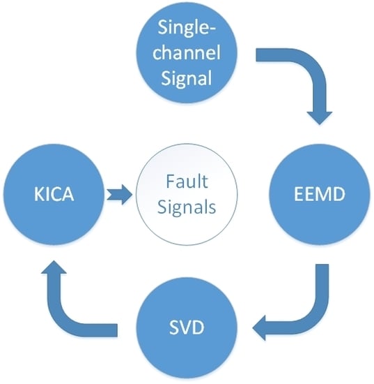
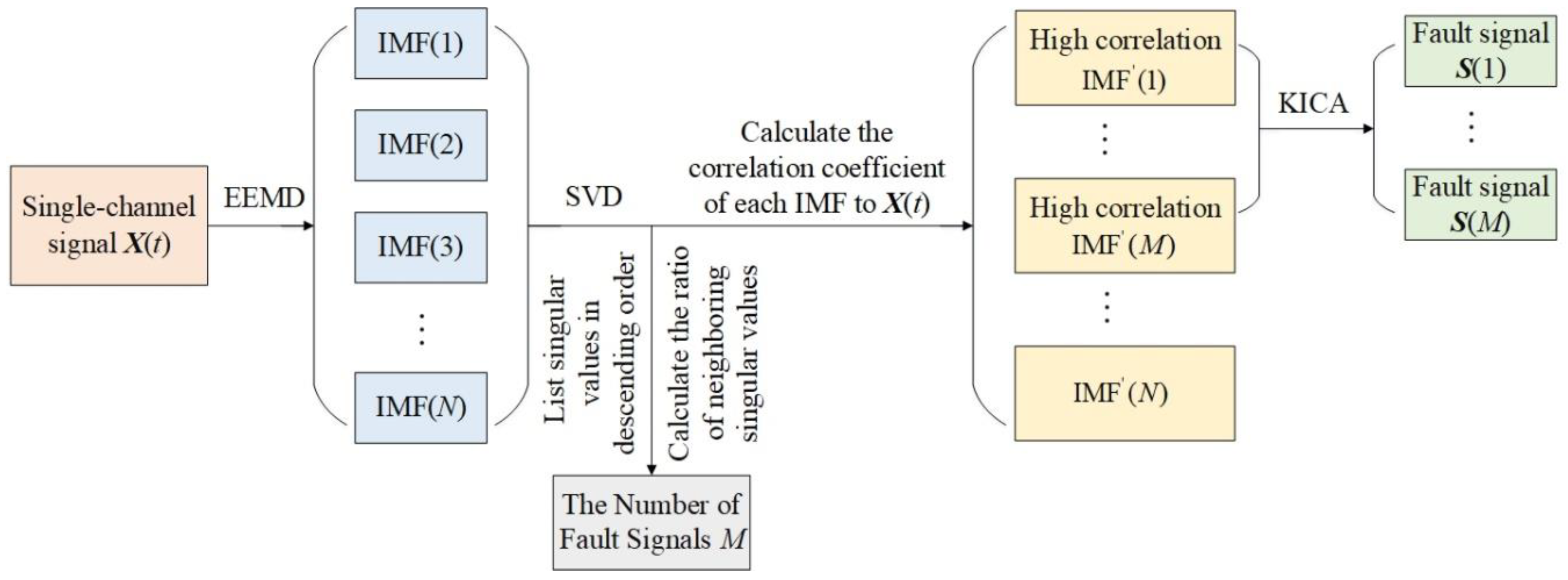
3. The Proposed Method

In this paper, a fault-feature extraction method of rotating machinery based on EEMD-based KICA is proposed. Its advantage is that it can estimate the number of fault signals of a single-channel vibration signal and can extract fault features clearly. This method only needs to input a single-channel signal, and the outputs are fault signals and number, without artificial selection. The procedure of the proposed method has been summarized in Figure 1. The detailed procedure is described as follows:

Step 1: The collected single-channel signal $\mathit{X}(t)$ is decomposed with EEMD, and all IMFs can be obtained. Then, the multidimensional observation signal can be formed with all IMFs.

Step 2: The observation signal is decomposed with SVD first. Then, singular values are listed in descending order. Next, the ratio of neighboring singular values is calculated. Finally, the sequence number of the maximum ratio will be the number of fault signals M.

Step 3: Calculate the correlation coefficient of each IMF to $\mathit{X}(t)$ and select the top M IMFs with the highest correlation to form a new observation signal. Finally, use KICA to extract the fault signals from the new observation signal.

4. Application and Validation

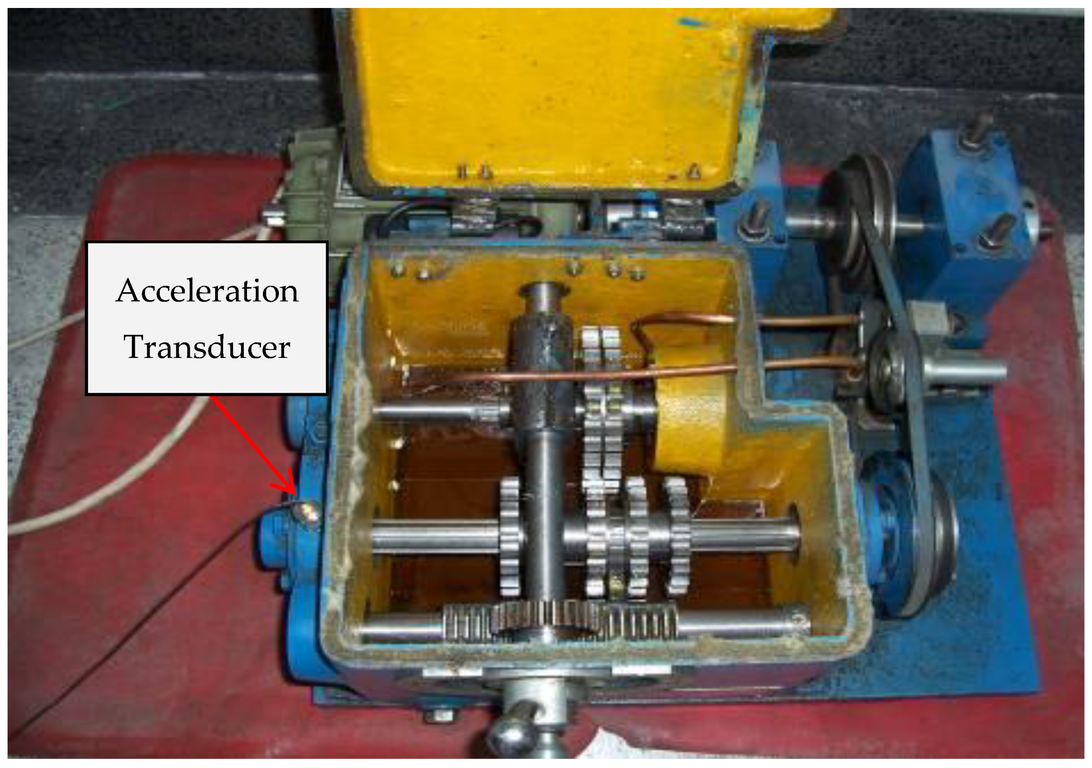
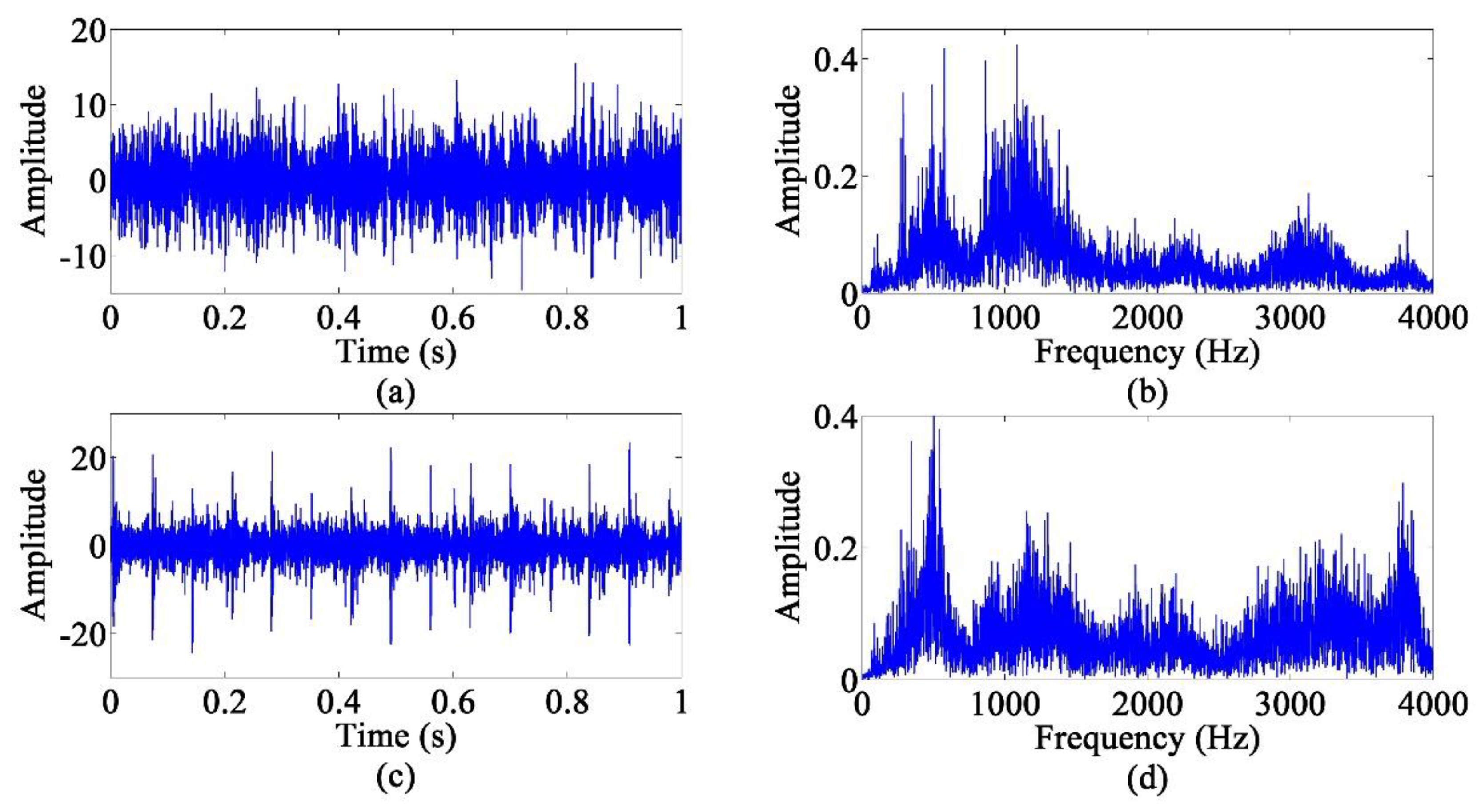
4.1. Experimental Analysis of Faulty Gear

In order to verify the effectiveness of the proposed method with faulty gear, the collected vibration signal of faulty gear is analyzed. The experimental device is shown in Figure 2. The whole device is driven by a 550 W (220 V, 50 Hz) AC motor that drives the shaft system with couplings. There are two rolling bearings on the shaft system. The shaft section between two bearing seats is equipped with a belt wheel, and the belt drives the active gear shaft of the gear box. One acceleration transducer is installed vertically on the shell near the shaft. The sampling frequency $f_s=8192 \mathrm{Hz}$ and the sampling point number is 8192. The motor speed is 850 rpm, that is, the rotation frequency $f_r=14.2 Hz$. The number of gear teeth $Z=20$. According to $f_c=Z\times f_r$, the gear mesh frequency $f_c=283.3 \mathrm{Hz}$.

In this experimental analysis, the collected vibration signal of a broken tooth fault is selected, and the number of the broken tooth $Z_b=1$. From experience, when the gear is affected by a broken tooth fault, the rotation frequency $f_r$ and its frequency multiplication will be the main features in the frequency domain, and the frequency $f_z=Z_b\times f_c$ will also exist. The time-domain waveforms and amplitude spectra obtained by fast Fourier transform (FFT) [23] of a healthy signal and faulty signal are shown in Figure 3.

The fault features of the collected signal cannot be found in Figure 3. The performance of feature extraction of a broken tooth fault with wavelets, EMD, VMD, EEMD and the proposed method are compared in the following section.

4.1.1. Wavelets

In this method, the collected signal is decomposed with five-layer Daubechies wavelet decomposition first, and then the amplitude spectra of each component can be obtained with FFT. The result in Figure 4 shows that the rotation frequency $f_r$ and its frequency multiplication are not extracted, and the frequency $f_z$ is also not extracted. Therefore, wavelets cannot extract the fault feature of a broken tooth.

4.1.2. EMD

In this method, the collected signal is decomposed with EMD first, and then the amplitude spectra of each IMF can be obtained with FFT. The result in Figure 5 shows that the rotation frequency $f_r$ and its frequency multiplication are not extracted, and the frequency $f_z$ is also not extracted. Therefore, EMD cannot extract the fault feature of a broken tooth.

4.1.3. VMD

In this method, the collected signal is decomposed with VMD first, and then the Hilbert envelope spectra (HES) [24] of each component signal can be obtained. The result in Figure 6 shows that the motor rotation frequency $f_r$ and its double frequency and triple frequency can be seen in each subfigure of Figure 6, and the frequency of 288 Hz, which is very close to $f_z$, can be seen in Figure 6b,d. However, the features are still not clear enough.

4.1.4. EEMD

In this method, the collected signal is decomposed with EEMD first, and then the Hilbert envelope spectra of each IMF can be obtained. The result in Figure 7 shows that the motor rotation frequency $f_r$ and its double frequency and triple frequency can be seen in each subfigure of Figure 7, and the frequency of 288 Hz, which is very close to $f_z$, can be seen in Figure 7a,b. However, the features are not clear enough, the amplitudes of other frequencies are very high and noise energy is still high.

4.1.5. The Proposed Method

In this method, the collected signal is decomposed with EEMD first, and then the number of fault signals can be estimated with SVD. The ratios of neighboring singular values are shown in

Table 1. The ratios of neighboring singular values.

Sequence Number	NSVR
1	6.254
2	2.561
3	2.033
4	1.875
5	1.262
6	0.801

.

As shown in Table 1, the sequence number of the maximum NSVR is 1. Therefore, the number of fault signals is 1. According to the correlation coefficient of each IMF, the observation signal is reconstructed with high-correlation IMFs. Finally, the fault signals can be extracted from the new observation signal with KICA. The Hilbert envelope spectra of the extracted fault signal is shown in Figure 8.

The result in Figure 8 shows that the motor rotation frequency $f_r=14 \mathrm{Hz}$ and its double frequency and triple frequency have been extracted clearly, and $f_z=283.3 \mathrm{Hz}$ is also extracted clearly. The amplitude of $f_r$ is much larger than $f_z$, so it can be clearly judged to be the broken tooth fault.

4.1.6. Results and Discussions

Compared with the methods of wavelets and EMD, the proposed method has a significantly better performance for the feature extraction of a single-channel vibration signal of faulty gear. Although VMD and EEMD can extract fault features, the noise energy is still very high. Compared with the method of EEMD, the noise energy has been reduced in the proposed method, which is efficient for fault-feature extraction.

4.2. Experimental Analysis of Faulty Rolling Bearing

In order to verify the validity of the proposed method for a faulty rolling bearing vibration signal, the test data from the bearing database of Case Western Reserve University are selected for analysis. The experimental device is shown in Figure 9. At the output terminal of the motor, one acceleration transducer is vertically installed on the shell of a supporting bearing to collect data.

The rolling bearing used in the test is SKF6205. The motor speed is 1180 rpm, that is, the rotation frequency $f_r=19.7 \mathrm{Hz}$. The sampling frequency $f_s=8192 \mathrm{Hz}$ and the number of sampling points is 8192. The inner and outer rings of the rolling bearing are respectively machined with tiny pitting pits of 0.28 mm in depth and 0.54 mm in diameter to simulate the faults of an inner ring and an outer ring. The fault frequency of the inner ring can be expressed as:

$$f_{ic}=\frac{1}{2}N(1+\frac{d}{D}\cos \alpha )f_r.$$

(12)

The fault frequency of the outer ring can be expressed as:

$$f_{oc}=\frac{1}{2}N(1-\frac{d}{D}\cos \alpha )f_r,$$

(13)

where $N$ is the number of rollers, $d$ is the diameter of the rollers, $D$ is the pitch diameter of the bearing, and $\alpha$ is the bearing’s contact angle. According to Equations (12) and (13), $f_{ic}=106 \mathrm{Hz}$ and $f_{oc}=70 \mathrm{Hz}$.

The time-domain waveform and amplitude spectra of a healthy signal and faulty signal are shown in Figure 10.

The fault features of the inner ring and outer ring cannot be found from the time-domain waveform and amplitude spectra in Figure 10. Therefore, the effectiveness of feature extraction via wavelets, EMD, VMD, EEMD and the proposed method are compared in the following section.

4.2.1. Wavelets

In this method, firstly, the observation signal is decomposed with six-layer Daubechies wavelet decomposition, and then the amplitude spectra of each component can be obtained with FFT. The result is shown in Figure 11. The frequency of 107 Hz, which is very close to $f_{ic}$, is extracted in Figure 11b, but $f_{oc}$ is not extracted. Therefore, wavelets cannot fully extract the fault feature of a rolling bearing.

4.2.2. EMD

In this method, the observation signal is decomposed with EMD first, and then the amplitude spectra of each IMF can be obtained with FFT. The result in Figure 12 shows that the fault features of the inner ring and outer ring are not extracted.

4.2.3. VMD

In this method, the observation signal is decomposed by VMD first, and then the Hilbert envelope spectra of each component signal can be obtained. The result is shown in Figure 13. In Figure 13a,b, the fault frequency of the outer ring, $f_{ic}=70 \mathrm{Hz}$, is extracted. The fault frequency of the inner ring, $f_{oc}=106 \mathrm{Hz}$, can be seen in Figure 13c. However, the amplitudes of other frequencies and the noise energy are still high.

4.2.4. EEMD

In this method, the observation signal is decomposed with EEMD first, and then the Hilbert envelope spectra of each IMF can be obtained. The result is shown in Figure 14. In Figure 14a, the fault frequency of the inner ring, $f_{ic}=106 \mathrm{Hz}$, is extracted. The fault frequency of the outer ring, $f_{oc}=70 \mathrm{Hz}$, can be seen in Figure 14b. However, the features are not clear enough, the amplitudes of other frequencies are very high and the noise energy is still high.

4.2.5. The Proposed Method

In this method, the observation signal is decomposed with EEMD first, and then the number of fault signals can be estimated with SVD. The ratios of neighboring singular values are shown in

Table 2. The ratios of neighboring singular values.

Sequence Number	NSVR
1	1.524
2	36.810
3	6.884
4	3.922
5	5.516
6	0.981

.

As shown in Table 2, the sequence number of the maximum NSVR is 2. Therefore, the number of fault signals is 2. According to the correlation coefficient of each IMF, the observation signal is reconstructed with high-correlation IMFs. Finally, the fault signals can be extracted from the new observation signal with KICA. The Hilbert envelope spectra of the extracted fault signals are shown in Figure 15.

In Figure 15b, the fault frequency of the inner ring, $f_{ic}=106 \mathrm{Hz}$, is extracted. The fault frequency of the outer ring, $f_{oc}=70 \mathrm{Hz}$, can be seen in Figure 15a. Furthermore, the features are extracted clearly.

4.2.6. Results and Discussions

Compared with the other four methods, the proposed method has a better performance for the feature extraction of a single-channel vibration signal of a faulty rolling bearing. The feature of fault frequency is more obvious and noise energy is obviously reduced. The experimental analysis of the faulty rolling bearing proves that our proposed method can estimate the number of fault signals and is efficient to extract the features of a single-channel signal with multiple faults.

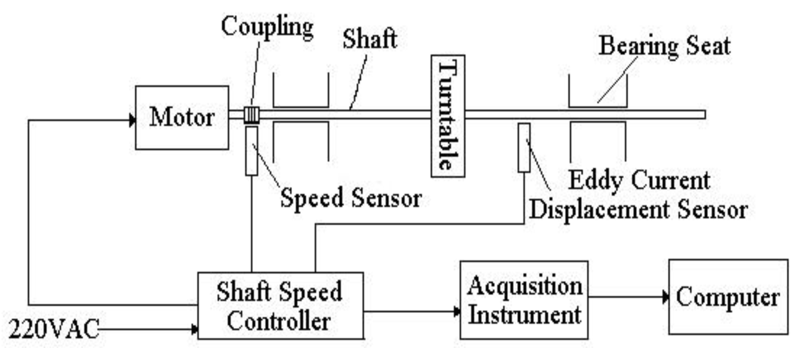
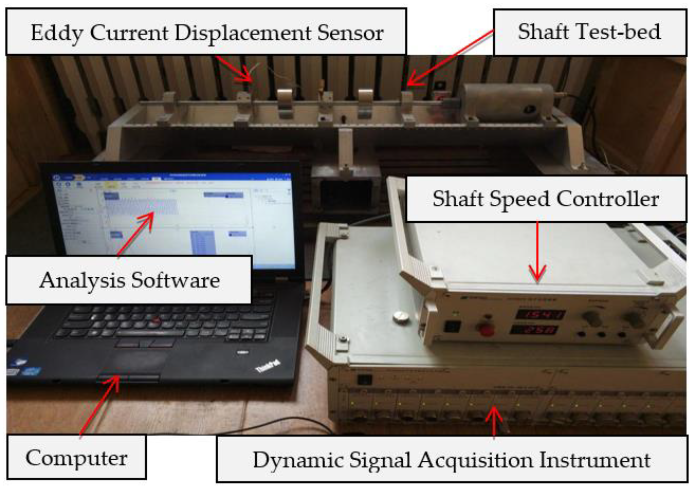
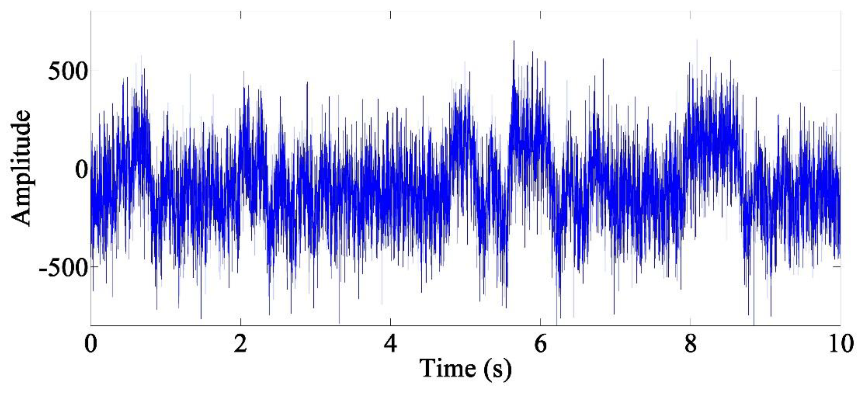
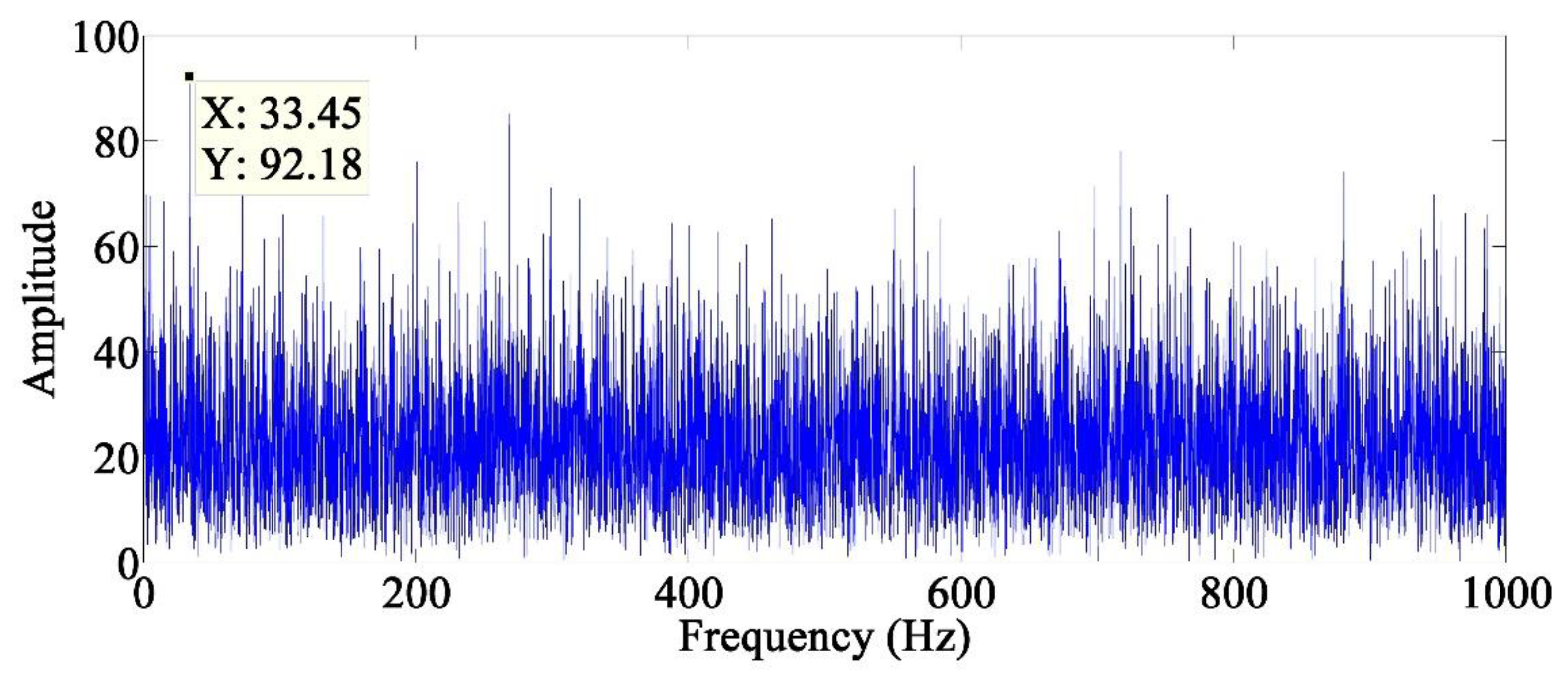
4.3. Experimental Analysis of a Faulty Shaft

A faulty-shaft experimental analysis is applied to verify the effectiveness of the proposed method. The schematic diagram of the test system is shown in Figure 16, and the test rig and signal acquisition system are shown in Figure 17. The test system includes a sensor, shaft test-bed, shaft speed controller, dynamic signal acquisition instrument, computer and analysis software. The sensor sends a radial vibration signal of the shaft into the dynamic signal acquisition instrument, and then converts the analog signal into a digital signal. Finally, the digital signal will be uploaded to analysis software of the computer to realize various analyses required by the user.

In this experimental analysis, the artificial imbalance fault and rub-impact fault are created. Only one eddy current displacement sensor is used to collect the mixed vibration signal of the faulty shaft. The sampling frequency is 1000 Hz and the number of sampling points is 10,000. The motor speed is 2000 rpm, that is, the rotation frequency $f_r=33.3 \mathrm{Hz}$. From experience, the feature of an imbalance fault causes the frequency $f_r$ alone in the frequency-domain. The feature of a rub-impact fault causes the frequency $f_r$ and 1/n of $f_r$, where n is equal to 2, 3, 4 or 5. The time-domain waveform of the collected signal is shown in Figure 18, and the amplitude spectra of the collected signal obtained with FFT is shown in Figure 19.

As can be seen in Figure 18, none of the periodic amplitude can be seen in the time domain. The frequency of 33.45 Hz, which is very close to $f_r$, can be seen in Figure 19, but the amplitude of other frequencies is very high and the noise energy is high.

In the proposed method, firstly, the collected single-channel vibration signal is decomposed with EEMD, and then the number of fault signals can be estimated with SVD. The ratios of neighboring singular values are shown in

Table 3. The ratios of neighboring singular values.

Sequence Number	NSVR
1	1.926
2	22.568
3	3.448
4	2.962
5	1.979
6	1.038

.

As shown in Table 3, the sequence number of the maximum NSVR is 2. Therefore, the number of fault signals is 2. Finally, high-correlation IMFs are selected to reconstruct a new observation signal, and then fault signals can be extracted with KICA. The Hilbert envelope spectra of the extracted fault signals are shown in Figure 20.

Both the frequencies of 33.45 Hz and 6.836 Hz can be found in Figure 20a, which can be considered the features of a rub-impact fault. Figure 20b only has the frequency of 33.45 Hz, which can be considered as the feature of an imbalance fault. Furthermore, the fault features are significantly obvious. It demonstrates that the proposed method has a good performance of fault-feature extraction of a faulty shaft with both the imbalance fault and the rub-impact fault.

5. Conclusions

The method with EEMD-based KICA has been proposed to improve the efficiency of fault-feature extraction of a single-channel vibration signal of rotating machinery in this paper. Its advantage is that it can estimate the number of fault signals of a single-channel vibration signal and extract the fault features clearly. This method only needs to input a single-channel signal, and the outputs are fault signals and number, without artificial selection. Through the experiment of faulty gear, a faulty rolling bearing and a faulty shaft, the results show that the proposed method makes the fault features more clear compared with wavelets, EMD, VMD and EEMD, which demonstrates its effectiveness for fault-feature extraction of rotating machinery.

Because this paper mainly studies the effectiveness of the new proposed method, mainly for offline signals, future studies will conduct online signal research, which requires attention to the problem of time consumption. Finally, this fault diagnosis method of rotating machinery is worth being evaluated with large industrial equipment.

References

1. Cheng, J.; Yang, Y.; Yang, Y. A rotating machinery fault diagnosis method based on local mean decomposition. Digit. Signal Process. 2012, 22, 356–366. [Google Scholar] [CrossRef]
2. Xu, T.; Yin, Z.; Cai, D.; Zheng, D. Fault diagnosis for rotating machinery based on Local Mean Decomposition morphology filtering and Least Square Support Vector Machine. J. Intell. Fuzzy Syst. 2017, 32, 2061–2070. [Google Scholar] [CrossRef]
3. Ciabattoni, L.; Ferracuti, F.; Freddi, A.; Monteriù, A. Statistical Spectral Analysis for Fault Diagnosis of Rotating Machines. IEEE Trans. Ind. Electron. 2017, 65, 4301–4310. [Google Scholar] [CrossRef]
4. Yan, R.; Gao, R.X.; Chen, X. Wavelets for fault diagnosis of rotary machines: A review with applications. Signal Process. 2014, 96, 1–15. [Google Scholar] [CrossRef]
5. Lin, J.; Zhang, A. Fault feature separation using wavelet-ICA filter. NDT E Int. 2005, 38, 421–427. [Google Scholar] [CrossRef]
6. Keshtan, M.N.; Khajavi, M. Bearings fault diagnosis using vibrational signal analysis by EMD method. Res. Nondestruct. Eval. 2015, 27, 155–174. [Google Scholar] [CrossRef]
7. Feng, Z.; Zhang, D.; Zuo, M.J. Adaptive Mode Decomposition Methods and Their Applications in Signal Analysis for Machinery Fault Diagnosis: A Review with Examples. IEEE Access 2017, 5, 24301–24331. [Google Scholar] [CrossRef]
8. Tabrizi, A.; Garibaldi, L.; Fasana, A.; Marchesiello, S. Early damage detection of roller bearings using wavelet packet decomposition, ensemble empirical mode decomposition and support vector machine. Meccanica 2015, 50, 865–874. [Google Scholar] [CrossRef]
9. Cheng, G.; Chen, X.; Li, H.; Li, P.; Liu, H. Study on planetary gear fault diagnosis based on entropy feature fusion of ensemble empirical mode decomposition. Measurement 2016, 91, 140–154. [Google Scholar] [CrossRef]
10. Dragomiretskiy, K.; Zosso, D. Variational Mode Decomposition. IEEE Trans. Signal Process. 2014, 62, 531–544. [Google Scholar] [CrossRef]
11. Li, K.; Su, L.; Wu, J.; Wang, H.; Chen, P. A Rolling Bearing Fault Diagnosis Method Based on Variational Mode Decomposition and an Improved Kernel Extreme Learning Machine. Appl. Sci. 2017, 7, 1004. [Google Scholar] [CrossRef]
12. Li, Z.; Jiang, Y.; Wang, X.; Peng, Z. Multi-mode separation and nonlinear feature extraction of hybrid gear failures in coal cutters using adaptive nonstationary vibration analysis. Nonlinear Dyn. 2016, 84, 295–310. [Google Scholar] [CrossRef]
13. Yang, Z.X.; Zhong, J.H. A Hybrid EEMD-Based SampEn and SVD for Acoustic Signal Processing and Fault Diagnosis. Entropy 2016, 18, 112. [Google Scholar] [CrossRef]
14. Shen, H.; Jegelka, S.; Gretton, A. Fast kernel-based independent component analysis. IEEE Trans. Signal Process. 2009, 57, 3498–3511. [Google Scholar] [CrossRef]
15. Zhang, Y.; Du, W.; Li, X. Observation and Detection for a Class of Industrial Systems. IEEE Trans. Ind. Electron. 2017, 64, 6724–6731. [Google Scholar] [CrossRef]
16. Chen, Q.; Liu, R. On the explanation of spatial smoothing in MUSIC algorithm for coherent sources. Int. Conf. Inf. Sci. Technol. 2011, 699–702. [Google Scholar] [CrossRef]
17. Yuan, X. Coherent Source Direction-Finding using a Sparsely-Distributed Acoustic Vector-Sensor Array. IEEE Trans. Aerosp. Electron. Syst. 2012, 48, 2710–2715. [Google Scholar] [CrossRef]
18. Cheng, W.; Zhang, Z.; He, Z. Information criterion-based source number estimation methods with comparison. Hsi-An Chiao Tung Ta Hsueh/J. Xi’an Jiaotong Univ. 2015, 49, 38–44. [Google Scholar]
19. Ridder, F.D.; Pintelon, R.; Schoukens, J.; Gilikin, D.P. Modified AIC and MDL model selection criteria for short data records. IEEE Trans. Instrum. Meas. 2005, 54, 144–150. [Google Scholar] [CrossRef]
20. Hill, E.R.; Xia, W.; Clarkson, M.J.; Desiardins, A.E. Identification and removal of laser-induced noise in photoacoustic imaging using singular value decomposition. Biomed. Opt. Express 2017, 8, 68–77. [Google Scholar] [CrossRef] [PubMed]
21. Sun, H.; Guo, J.; Fang, L. Improved singular value decomposition (TopSVD) for source number estimation of low SNR in blind source separation. IEEE Access 2017, 5, 26460–26465. [Google Scholar] [CrossRef]
22. Huang, N.E.; Shen, Z.; Long, S.R. The empirical mode decomposition and the Hilbert spectrum for nonlinear and non-stationary time series analysis. Proc. Math. Phys. Eng. Sci. 1998, 454, 903–995. [Google Scholar] [CrossRef]
23. Salih, A.L.; Gaeid, K.S.; Ping, H.W.; Khalid, M. Fault Diagnosis of Induction Motor Using MCSA and FFT. Electr. Electron. Eng. 2011, 60, 39–48. [Google Scholar]
24. Pan, M.C.; Tsao, W.C. Using appropriate IMFs for envelope analysis in multiple fault diagnosis of ball bearings. Int. J. Mech. Sci. 2013, 69, 114–124. [Google Scholar] [CrossRef]
Figure 1. The summarized procedure of the proposed method.
Applsci 08 01441 g001
Figure 2. The test rig of faulty gear.
Applsci 08 01441 g002
Figure 3. The time-domain waveforms and amplitude spectra of a healthy signal and faulty signal. (a) The time-domain waveform of a healthy signal. (b) The amplitude spectra of a healthy signal. (c) The time-domain waveform of a faulty signal. (d) The amplitude spectra of a faulty signal.
Applsci 08 01441 g003
Figure 4. The amplitude spectra of each component after five-layer wavelet decomposition. (a) The fifth layer of the low-frequency component. (b) The fifth layer of the high-frequency component. (c) The fourth layer of the high-frequency component. (d) The third layer of the high-frequency component.
Applsci 08 01441 g004
Figure 5. The amplitude spectra of each intrinsic mode function (IMF) after empirical mode decomposition (EMD). (a) IMF1. (b) IMF2. (c) IMF3. (d) IMF4.
Applsci 08 01441 g005
Figure 6. The Hilbert envelope spectra of each component signal after variational mode decomposition (VMD). (a) Component signal 1. (b) Component signal 2. (c) Component signal 3. (d) Component signal 4.
Applsci 08 01441 g006
Figure 7. The Hilbert envelope spectra of each IMF after ensemble empirical mode decomposition (EEMD). (a) IMF1. (b) IMF2. (c) IMF3. (d) IMF4.
Applsci 08 01441 g007
Figure 8. The Hilbert envelope spectra of the extracted fault signal after kernel-independent component analysis (KICA).
Applsci 08 01441 g008
Figure 9. The test rig of a faulty rolling bearing.
Applsci 08 01441 g009
Figure 10. The time-domain waveform and amplitude spectra of a healthy signal and faulty signal. (a) The time-domain waveform of a healthy signal. (b) The amplitude spectra of a healthy signal. (c) The time-domain waveform of a faulty signal. (d) The amplitude spectra of a faulty signal.
Applsci 08 01441 g010
Figure 11. The amplitude spectra of each component after six-layer wavelet decomposition. (a) The sixth layer of the low-frequency component. (b) The sixth layer of the high-frequency component. (c) The fifth layer of the high-frequency component. (d) The fourth layer of the high-frequency component.
Applsci 08 01441 g011
Figure 12. The amplitude spectra of each IMF after EMD. (a) IMF1. (b) IMF2. (c) IMF3. (d) IMF4.
Applsci 08 01441 g012
Figure 13. The Hilbert envelope spectra of each component signal after VMD. (a) Component signal 1. (b) Component signal 2. (c) Component signal 3. (d) Component signal 4.
Applsci 08 01441 g013
Figure 14. The Hilbert envelope spectra of each IMF after EEMD. (a) IMF1. (b) IMF2. (c) IMF3. (d) IMF4.
Applsci 08 01441 g014
Figure 15. The Hilbert envelope spectra of the extracted fault signals after KICA. (a) The first fault signal. (b) The second fault signal.
Applsci 08 01441 g015
Figure 16. The schematic diagram of the test system.
Applsci 08 01441 g016
Figure 17. The test rig and signal acquisition system of a faulty shaft.
Applsci 08 01441 g017
Figure 18. The time-domain waveform of the collected signal.
Applsci 08 01441 g018
Figure 19. The amplitude spectra of the collected signal.
Applsci 08 01441 g019
Figure 20. The Hilbert envelope spectra of the extracted fault signals after KICA. (a) The first fault signal. (b) The second fault signal.
Applsci 08 01441 g020