Lamb Wave Local Wavenumber Approach for Characterizing Flat Bottom Defects in an Isotropic Thin Plate


1
School of Communication and Information Engineering, Shanghai University, Shanghai 200444, China
2
School of Urban Railway Transportation, Shanghai University of Engineering Science, Shanghai 201620, China
*
Author to whom correspondence should be addressed.
Appl. Sci. 2018, 8(9), 1600; https://doi.org/10.3390/app8091600
Submission received: 28 June 2018
/
Revised: 18 July 2018
/
Accepted: 24 July 2018
/
Published: 10 September 2018
(This article belongs to the Special Issue Ultrasonic Guided Waves)
Abstract
:This paper aims to use the Lamb wave local wavenumber approach to characterize flat bottom defects (including circular flat bottom holes and a rectangular groove) in an isotropic thin plate. An air-coupled transducer (ACT) with a special incidence angle is used to actuate the fundamental anti-symmetric mode (A0). A laser Doppler vibrometer (LDV) is employed to measure the out-of-plane velocity over a target area. These signals are processed by the wavenumber domain filtering technique in order to remove any modes other than the A0 mode. The filtered signals are transformed back into the time-space domain. The space-frequency-wavenumber spectrum is then obtained by using three-dimensional fast Fourier transform (3D FFT) and a short space transform, which can retain the spatial information and reduce the magnitude of side lobes in the wavenumber domain. The average wavenumber is calculated, as a real signal usually contains a certain bandwidth instead of the singular frequency component. Both simulation results and experimental results demonstrate that the average wavenumber can be used not only to identify shape, location, and size of the damage, but also quantify the depth of the damage. In addition, the direction of an inclined rectangular groove is obtained by calculating the image moments under grayscale. This hybrid and non-contact system based on the local wavenumber approach can be provided with a high resolution.
1. Introduction
Lamb waves have shown great potential for structural health monitoring (SHM) in plate-like structures [1]. Their attractive features include sensitivity to a variety of damage types and the capability of traveling relatively long distances [2]. Damage imaging methods based on Lamb waves have been widely studied by many researchers, such as delay-and-sum (DAS) imaging [3,4], time reversal focusing imaging [5,6], diffraction tomography imaging [7], and ultrasonic phased array [8].
Lamb waves are dispersive and multimodal [9]. Moreover, the propagating Lamb waves may include incident, reflected, and converted waves when they encounter a sudden thickness variation [10,11], such as circular flat bottom holes and rectangular grooves. Obviously, various wave modes make the interpretation of Lamb waves very difficult [12].
In previous literature, the mode identification and separation of Lamb waves have been widely investigated in the time domain, time-frequency domain, and frequency-wavenumber domain [13,14]. Short-time Fourier transform (STFT) with a sliding window can make the variant distribution of the energy spectrum act as a function of time, which is capable of identifying Lamb wave mode [15]. Frequency-wavenumber analysis based on two-dimensional fast Fourier transform (2D FFT) is a useful approach to distinguish multiple modes. Moreover, the individual Lamb mode can be separated by a 2D band-pass filter [16]. It should be noted that the spatial information is also lost [17].
Compared with the above methods, the local wavenumber approach combined with a spatial window is viewed as an effective way to obtain the space-frequency-wavenumber spectrum. Furthermore, the spatial information can be reserved and the local features of the material can be clearly characterized, including, for instance, the thickness distribution of the material.
Many researchers have tried to utilize the above techniques for SHM. Yu et al. adopted a short space 2D Fourier transform to obtain the frequency-wavenumber spectrum at various spatial locations. Consequently, a through-thickness crack of an aluminum plate was discriminated by analyzing the space-frequency-wavenumber spectrum [18], but the size of the crack was not quantified. In another study, Yu et al. proved that spatial wavenumber imaging method was able to characterize the location and length of a crack. However, multiple cracks and cracks with various orientations were not researched in their work [19]. Rogge et al. utilized the local wavenumber analysis to characterize the impact damage in composite laminates [20]. The location of a preset delamination was clearly characterized, while its depth was not quantified.
Rao et al. reconstructed the thickness distribution of a liquid loaded plate by using an ultrasonic guided wave tomography method based on full waveform inversion (FWI) [21,22]. It was noted that the remaining wall thickness was reconstructed with high accuracy and resolution. Chronopoulos et al. adopted an inverse wave and finite element approach to recover the thickness and density, as well as all independent mechanical characteristics of layered composite structures [23]. However, one drawback of this method is that it is not efficient, as the inversion process is complicated and time-consuming. Therefore, a rapid method for SHM is desired.
Air-coupled ultrasonic inspection is a promising non-contact method for the rapid, non-contact inspection of materials [24,25]. The main advantages of this technique are the absence of any contact and the ability to generate a relatively pure Lamb wave mode when an appropriate incidence angle is adopted. The laser Doppler vibrometer (LDV) based on the Doppler effect has a high spatial resolution in obtaining the propagating Lamb waves [26]. Harb and Yuan accomplished the target of actuating the pure A0 mode (anti-symmetric mode) in an isotropic aluminum plate by employing an air-coupled transducer (ACT) and an LDV [27].
A hybrid non-contact system composed of an ACT and an LDV is presented in this paper. The local wavenumber approach is adopted to acquire the average wavenumber distribution of an isotropic thin plate, which contains circular flat bottom holes or a rectangular groove. The main goal is not only to extract defect features in location, size, and shape, but also quantify the depth of the damage by combining the wavenumber with the phase velocity dispersion curve. The direction of a rectangular groove can be attained by calculating the image moments under grayscale. Several factors which can affect test quality are analyzed in the discussion section. Moreover, the solutions are presented when the proposed approach is applied for an unknown damage.
This paper is organized with seven sections, including this introduction. Section 2 illustrates the theory of the local wavenumber approach. Section 3 presents the results of tests performed on numerically simulated examples. Experimental results are explicated in Section 4. Section 5 concludes the discussion. Section 6 provides recommendation for future research. Section 7 summarizes the main work.
2. Theory for the Local Wavenumber Approach
2.1. Sound Field Transmission and Reception
The A0 mode is the appropriate Lamb wave mode for characterizing circular flat bottom holes and a rectangular groove in an isotropic thin plate, as the phase velocity of the A0 mode is sensitive to the thickness-frequency product. First of all, a special incidence angle can be easily calculated based on Snell’s law. Then, the fundamental anti-symmetric mode (A0) can be actuated by an ACT with this special incidence angle. A scanning grid is predefined before using a non-contact LDV to measure the velocities of the desired mode. Obviously, the velocity is a function of both time and space. Figure 1 shows the theoretical dispersion curves obtained by a commercial software package called Disperse (version 2.0.20a, Imperial College London, London, UK) [28]. In this paper, the incidence angle is set at 12.75°, which is suitable for an ACT to actuate the A0 mode in an aluminum plate with the frequency-thickness product of 0.3 MHz·mm. Figure 2 shows a schematic diagram, which is used for describing the process of sound field transmission and reception.
2.2. Identification and Separation of Lamb Wave Modes in the Wavenumber Domain
Only the fundamental anti-symmetric mode (A0) can be actuated by ACT with the special incidence angle; however, mode conversion still exists due to the interaction between the Lamb wave and the flat bottom defects. The received Lamb wave signals usually comprise the incident, reflected, and converted wave modes. By using three-dimensional fast Fourier transform (3D FFT) [29], the full wavefield data can be transformed into the wavenumber domain, where various wave modes can be distinguished.
The entire wavefield signals are filtered by the wavenumber domain filter for the purpose of removing any modes other than the A0 mode.
These filtered signals in the wavenumber domain should be transformed back into the time domain by using three-dimensional inverse fast Fourier transform (3D IFFT). is the filtered wavefield.
2.3. Acquisition of the Average Wavenumber
A spatial window is used for reducing the magnitude of the side lobes. It should be noted that the spatial window size is at least twice the wavelength of the A0 mode in this paper. The centered coordinate of this spatial window is located at . Under this circumstance, the process of obtaining the average wavenumber is clearly illustrated as below.
First, a short space transform is conducted in order to retain the spatial information and reduce the magnitude of side lobes in the wavenumber domain. Specifically, the wavefield data is multiplied by a spatial window to produce the windowed dataset . The spatial window is non-zero for only a short period in space. The Hanning window is usually adopted [30].
where and can be expressed as:
Here, denotes the wavelength of the Lamb wave. is the window length. These signals processed with the spatial window are transformed into the spatial-frequency-wavenumber domain by using 3D FFT.
The weight of must be considered before calculating the local wavenumber , as presented in the following equation:
where is the Euclidean norm of the 2D wavenumber range [31]. The average wavenumber over the selected frequency band is calculated because a real signal usually contains a certain bandwidth instead of the singular frequency component. The average wavenumber of each point can be obtained by changing the centered coordinate of this spatial window and repeating the above steps. The flow chart of the local wavenumber approach is shown in Figure 3.
2.4. Depth Reconstruction
The average wavenumber at each point can be obtained by the local wavenumber approach. Hence, the phase velocity can be calculated as below:
The relationship between the phase velocity and the plate thickness can be gained from the phase velocity dispersion curve shown in Figure 1a. Consequently, the plate thickness of the target area can be reconstructed according to this relationship. Then, the depth distribution can be written as:
where is the thickness of the pristine plate. In order to evaluate the depth, the maximum depth error is defined as below:
Here, denotes the maximum value of the reconstructed depth and is the actual value.
3. Finite Element Simulation
3.1. Finite Element Model
A commercial software package called PZFlex was used to create the finite element model, which is shown in Figure 4. PZFlex is the time domain finite element method (FEM). The complex acoustic wave propagation in a three-dimensional model can be simulated by using this method [32]. The upper and bottom surfaces of the model are free, while the remaining four sides are absorbing. The size of the 6061-T6 aluminum plate is 400 mm × 400 mm × 1.5 mm, and the other material properties are listed in Table 1. The incident point of the ACT is (100, 200), and its incidence angle is set at 12.75°, which is suitable to actuate the A0 mode on aluminum with the frequency-thickness product of 0.3 MHz·mm. The damage located at the middle of the plate is a circular flat bottom hole with a diameter of 10 mm and a depth of 1 mm. This damage is surrounded by a rectangular scanning area (60 mm × 60 mm), which is divided into 121 × 121 points with a spatial interval of 0.5 mm. The spatial interval should not be more than half of the wavelength according to the sampling theorem. In our test, the phase velocity of the A0 mode is about 1551 m/s, and the central frequency of the received signal is 200 kHz. Therefore, the wavelength of the A0 mode is 7.775 mm ( = 1511/200 = 7.775 mm). The sampling interval is only 0.5 mm (). Apparently, the sampling interval satisfies the sampling theorem and can provide a good spatial resolution. The out-of-plane velocities over the scanning area are recorded by the LDV.
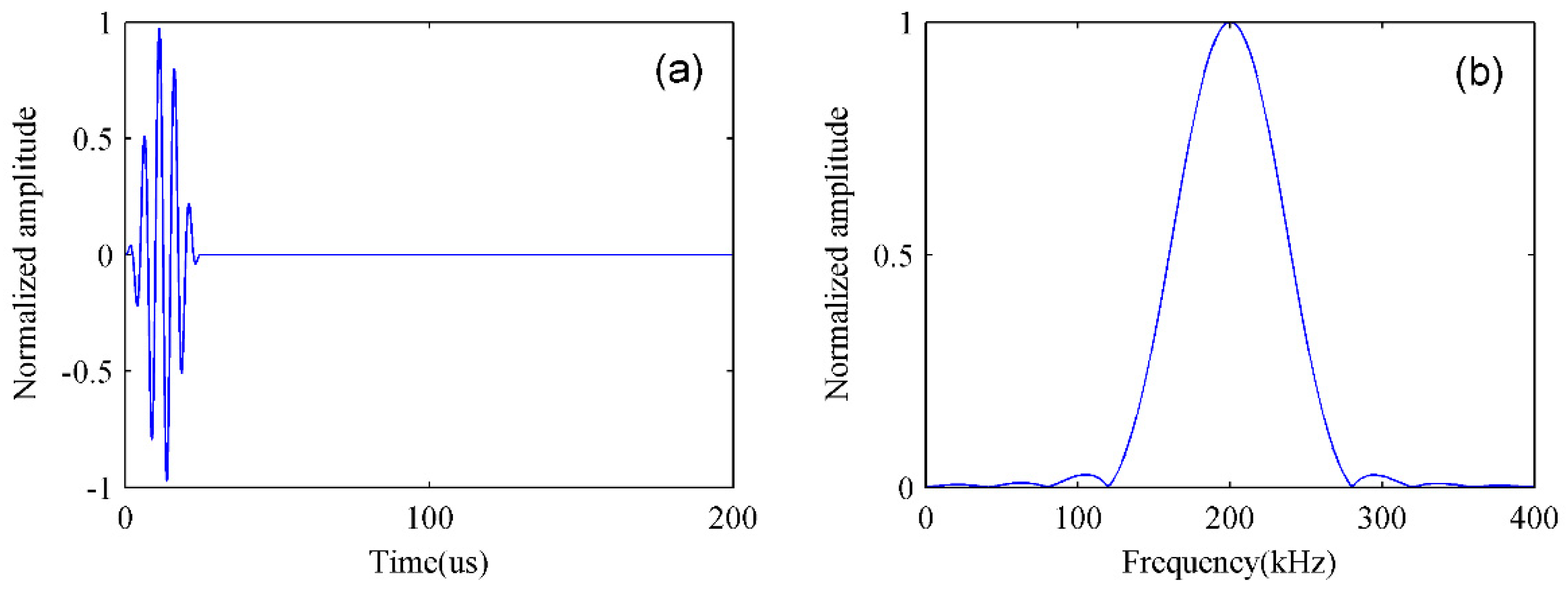
In this paper, a five-cycle sinusoidal tone burst modulated by a Hanning window with a central frequency of 200 kHz is applied as the excitation signal, which is shown in Figure 5. Eleven specimens listed in Table 2 are used to evaluate the performance of the local wavenumber approach from different aspects.
Case 1 and Case 2 are used to evaluate the performance of the proposed method when the circular flat bottom hole changes in depth.
Case 1 and Case 3 are used to evaluate the performance of the proposed method when the circular flat bottom hole changes in radius.
Case 4 to Case 7 are used to study the impacts caused by the excitation source position and the distance among adjacent defects. The excitation source in Case 4 and Case 5 is located at (100, 200), while it is located at (200, 100) in Case 6 and Case 7. The gap between the two flat bottom holes is 20 mm in Case 4 and Case 6, while it is 10 mm in Case 5 and Case 7.
Case 8 and Case 9 are used to investigate whether the impact which the big hole exerts on the small one is connected with their positions relative to the excitation source when they are in the same line.
Case 10 and Case 11 are used to identify the direction of the rectangular groove.
3.2. FEM Results
3.2.1. Mode Separation
The interactions between Lamb waves and the damage have been analyzed by many researchers. Bhuiyan et al. adopted the wave damage interaction coefficient (WDIC) to investigate the scattering of Lamb waves and demonstrated that the damage in the plate acted as a non-axisymmetric secondary source [33]. In another report, Bhuiyan et al. described the 3D interaction (frequency, incident direction, and azimuth direction) of Lamb waves with the damage [34]. Testoni et al. adopted a wavenumber filter to filter out the main wavefield generated by the acoustic source. Thus, the wave scattered by the delamination can be clearly observed in the filtered signal [35]. In this paper, Case 1 is taken as an example to describe the interaction between Lamb waves and the damage; moreover, the mode separation is introduced in detail.
The snapshots of the Lamb waves are shown in Figure 6. It can be observed that only the A0 mode can be actuated by an ACT with a special incidence angle. However, the S0 mode will be generated when the A0 mode encounters a flat bottom defect. Following this, the incident A0, reflected A0, transmitted A0, and S0 mode will coexist for a long time. It is worth noting that the amplitude of the S0 mode is very low.
The Lamb wave propagation was analyzed in detail. The next section will be focused on mode separation. The frequency-thickness product is 0.3 MHz·mm at the undamaged area. Under this situation, the theoretical wavenumbers of the A0 mode and S0 mode are 0.8102 rad/mm and 0.2312 rad/mm, respectively. The frequency-thickness product is only 0.1 MHz·mm at the damage. Hence, the theoretical wavenumbers of the A0 mode and S0 mode are 1.3082 rad/mm and 0.2311 rad/mm, respectively. Apparently, the wavenumber of the A0 mode changes more obviously than that of the S0 mode when the thickness changes. Figure 7 shows the mode separation by using 3D FFT and the wavenumber domain filtering technique. The wavenumber spectrum is obtained at a frequency of 200 kHz. The images are given in dB scale so that the wavenumber spectrum can be clearly visualized. The wavenumber spectrum for the pristine plate is shown in Figure 7a. The wavenumber spectrum for the damaged plate is shown in Figure 7b. The high-pass filter in wavenumber domain is shown in Figure 7c. The filtered wavenumber spectrum is shown in Figure 7d. By comparing the wavenumber spectrum in Figure 7a,b, we can confirm the fact that the A0 mode has interacted with the defect. In addition, the S0 mode generated by mode conversion is very weak, as the amplitude of the S0 mode is much lower than that of the A0 mode in the time domain.
Generally, a band-pass filter should be applied to reserve the A0 mode according to the theory of the local wavenumber approach. However, the wavenumber distribution of the A0 mode is wide in our test, while the wavenumber distribution of the S0 mode is very narrow. Moreover, the intensity of the S0 mode is weak. Therefore, it is easy to design a high-pass filter rather than a band-pass filter. The high-pass filter should ensure that the wavenumbers of the A0 mode are included in the pass band.
3.2.2. FEM Results of a Circular Flat Bottom Hole
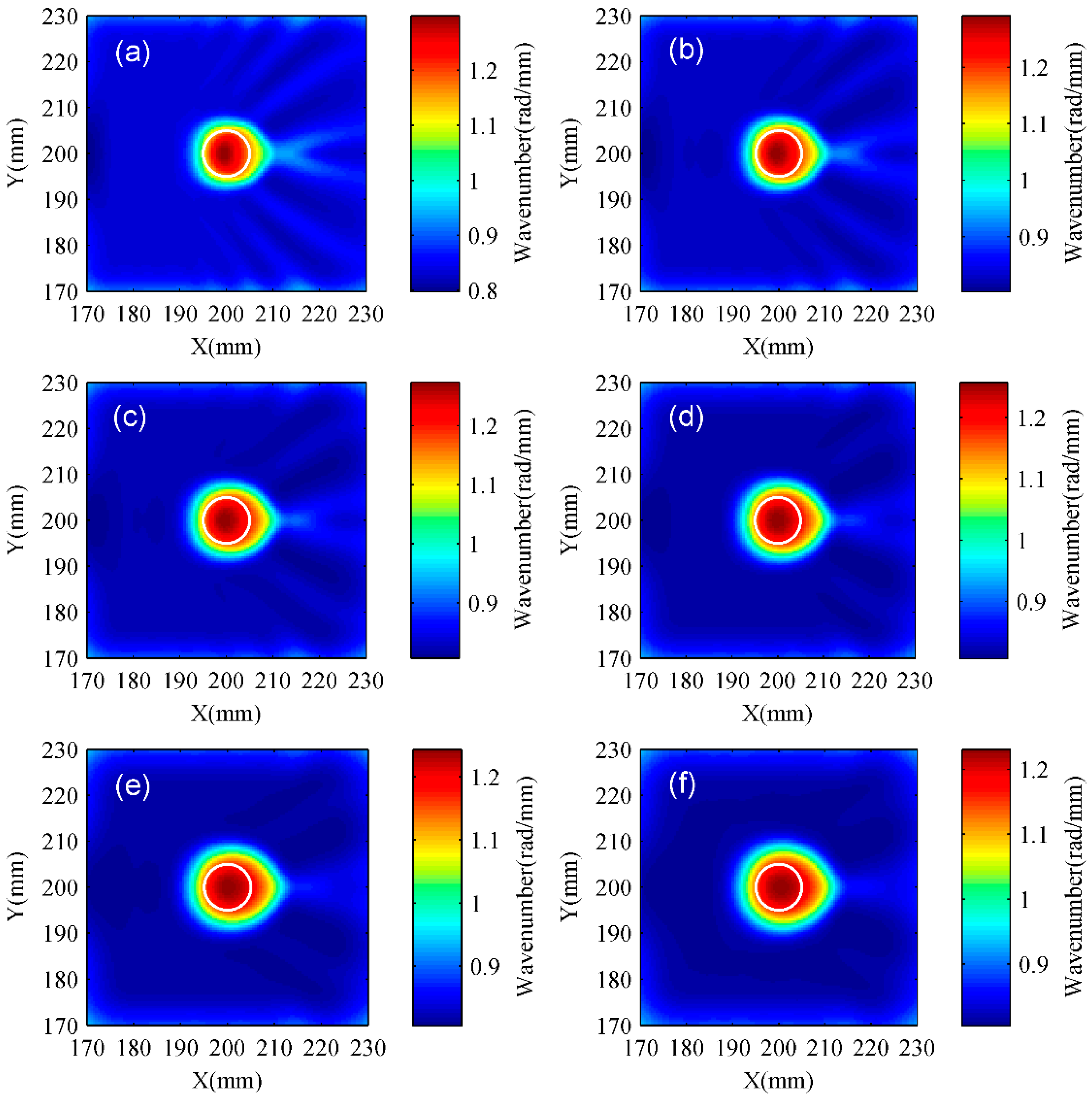
In this paper, the wavelength of the A0 mode is 7.775 mm. Therefore, the window radius () should be larger than 7.775 mm. It is assumed that the window radius is 8 mm. The average wavenumber can be obtained using Equation (12). Figure 8 shows the acquisition of the average wavenumber for Case 1. The frequency interval is 15 kHz. It can be seen that the average wavenumber contributes to improve the test quality at the scanning boundary by comparing Figure 8d,h. Moreover, lower image noise is seen in the image when the average wavenumber is adopted.
In fact, the best test result is not always obtained under the condition in which the window radius is equal to the wavelength. It is meaningful to analyze the test results under various window radii in order to find the optimum size. The test results shown in Figure 9 indicate that the damage region characterized by the proposed approach will expand as the window radius increases. Meanwhile, the maximum wavenumber attained under the various radii will decrease as the window radius increases, which is shown in Figure 10. It is only the window radius of 8 mm that can make the identified damage region match well with its actual size. Therefore, 8 mm is the optimum size. All of the test results were obtained under this condition.
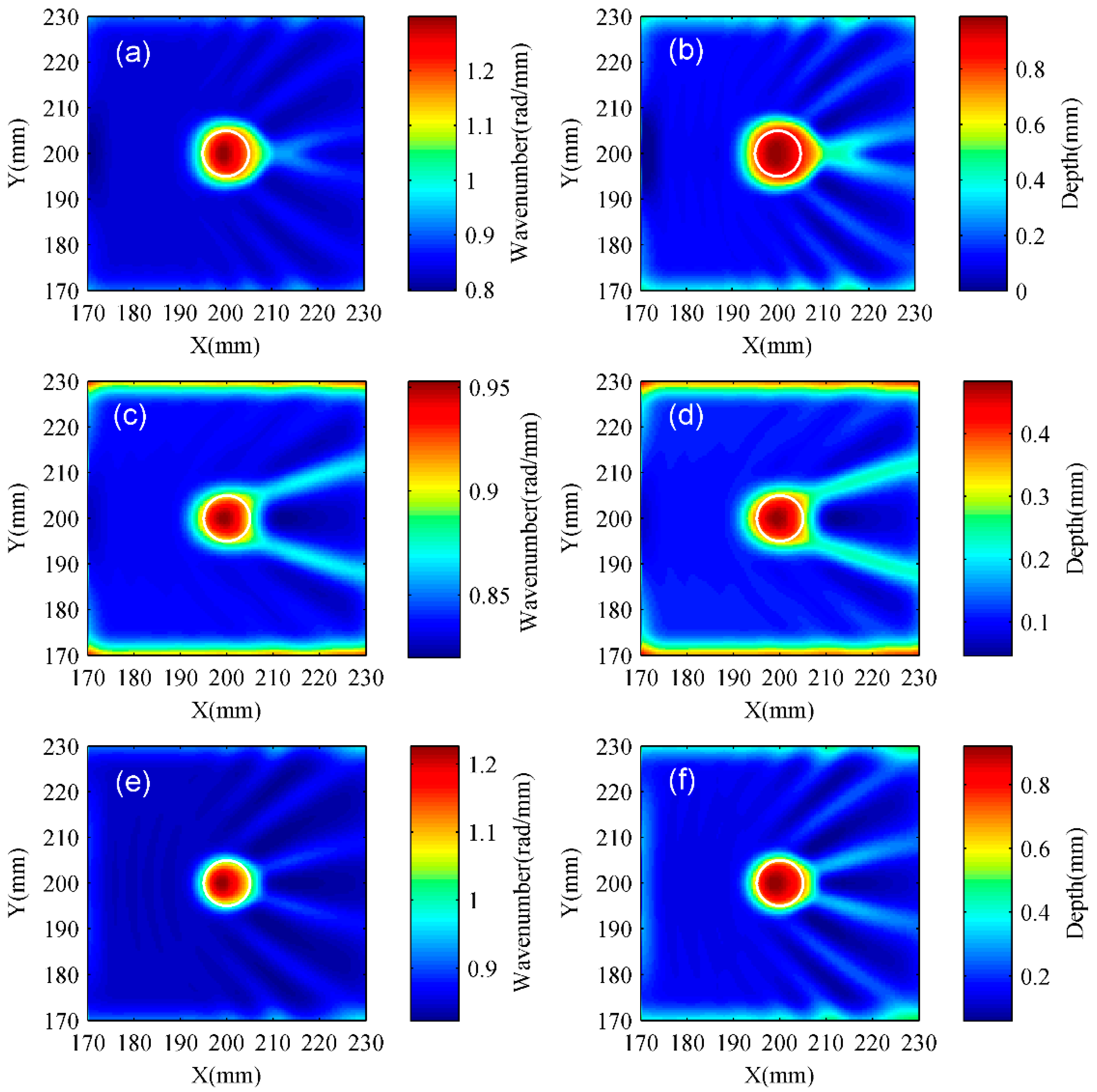
Case 1 and Case 2 only contain a circular flat bottom hole with the same radius and different depths. Case 1 and Case 3 only contain a circular flat bottom hole with different radii and the same depth. The specimen parameters are listed in Table 2. The simulation results of Case 1 to Case 3 are shown in Figure 11. The size and shape of the defect can be clearly visualized. The depth estimations are shown in Table 3. The depth error of the deep hole is 1.13%, while it reaches 3.26% for the shallow hole. Apparently, the depth estimation of the deep hole is more accurate than that of the shallow one. The depth error of the big hole is 1.13%, while it reaches 8.17% for the small one. Hence, the depth estimation of the big hole is more accurate than that of the small one.
3.2.3. FEM Results of Two Circular Flat Bottom Holes with the Same Radius and Depth
Case 4 to Case 7 contain two circular flat bottom holes with the same radius and depth, but the excitation source location and the gap between two defects are different. The specimen parameters are listed in Table 2. The simulation results of Case 4 to Case 7 are shown in Figure 12. It is observed that the shape and location of the defects are recognizable. The two holes exhibit a symmetrical distribution when the excitation source is located at (100, 200). In this condition, the better result appears under a big gap between the defects. The two holes and the excitation source are in the same line when the excitation source is located at (200, 100). In this condition, it can be noticed that the hole far away from the excitation source seems smaller than the near one. Moreover, the closer the defects are, the more obvious the effect is. Table 4 shows that the depth errors of Case 4 to Case 7 are all within 2%.
3.2.4. FEM Results of Two Circular Flat Bottom Holes with Different Radius and the Same Depth
Two circular flat bottom holes with different radii and the same depth are used in Case 8 and Case 9. It is important to note that these defects and the excitation source are in the same line, which means that the defects have the different positions relative to the excitation source. The specimen parameters are listed in Table 2. Simulation results are shown in Figure 13. It can be seen that the shape and location of two holes can be identified, which demonstrates that the local wavenumber approach has a high resolution even in distinguishing adjacent defects. Table 5 shows the depth evaluations of Case 8 and Case 9. The depth error of the big hole is within 1%, while the depth error of the small one is in the range of 4% to 9%. Thus, the depth estimation of the big hole is more accurate than that of the small one. Besides, the relative position is also taken into consideration. The depth error of the small hole is 8.17% when it is in front of the big one. Apparently, this level is equivalent to that of Case 3. However, the depth error of the small hole is reduced to 4.76% when it is behind the big one. This indicates that the impact which the big hole exerts on the small one is related to their positions when they and the excitation source are in the same line.
3.2.5. FEM Results of an Inclined Rectangular Groove
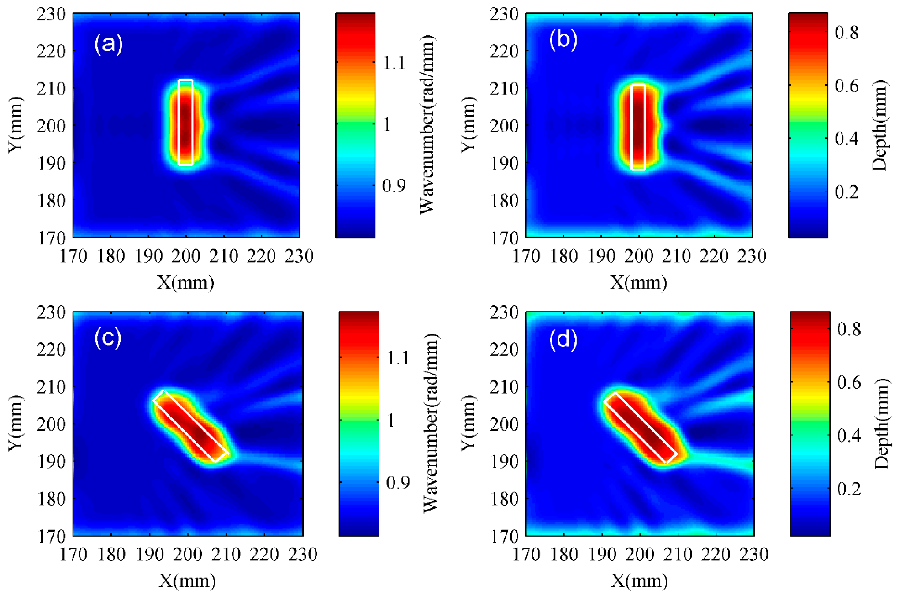
Case 10 is a rectangular groove with an inclined angle of 90°. Case 11 is a rectangular groove with an inclined angle of 135°. The specimen parameters are listed in Table 2. The simulation results of Case 10 and Case 11 are shown in Figure 14. The damage shape can be clearly visualized. It should be noted that the length of this defect is a little shorter than the actual value, while its width is obviously larger than the actual value. In addition, the orientation of the rectangular groove can be easily obtained and the computational process is introduced as below.
In image processing, computer vision, and related fields, an image moment is a certain particular weighted average (moment) of the image pixels’ intensities. Image moments and moment invariants are useful to describe global features in image processing [36]. Image moments are calculated under grayscale in order to distinguish the direction of the rectangular groove. denotes the pixel intensity of the gray value, where x, y are the row and column of the pixel matrix, respectively. The gray image must be processed by a threshold as we focus attention on the area where the rectangular groove is likely to exist rather than the whole area. is the pixel intensity obtained by setting a threshold at the level of −3 dB. The zero moment is shown in Equation (16). The first moment is shown in Equation (17). The second moment is shown in Equation (18). These image moments can be used to extract image features [37].
, , and are used to obtain the centroid coordinates of the feature image [38]. The calculation formulas are written as below.
The spindle orientation of the feature image can be obtained by calculating an angle, which is shown in the following equation.
where , , and can be given by the following equations:
Figure 15 shows the orientation of an inclined rectangular groove. The depth and angle evaluations are shown in Table 6. It is easy to find that the angle errors of Case 10 and Case 11 only reach 0.00% and 0.12%, respectively, while the depth errors of Case 10 and Case 11 rise to 12.95% and 13.60%, respectively. One reasonable explanation is clarified in the discussion section.
4. Experimental Verification
4.1. Experimental Setup
The experimental system is composed of an ACT, an LDV, an ultrasonic power device, a signal amplifier, a digital phosphor oscilloscope, and a data acquisition interface. The ACT is a piezoelectric ceramic-based transducer with a 200 kHz center frequency, and a bandwidth of ±25% of the center frequency. The incidence angle is set at 12.75°, which is suitable for the ACT to actuate the A0 mode. The LDV is employed to measure the out-of-plane velocity on the surface of the plate. The sampling frequency is set at 500 MHz. The signal should be executed at a suitable time when the waveform displayed on the oscilloscope tends to be stable. Each measurement is repeated 10 times in order to reduce the measurement error. The received signals need be amplified by a wideband amplifier for the purpose of improving the signal-to-noise ratio. The gain of the signal amplifier is 60 dB. Moreover, it can be adjusted according the central frequency of the excitation signal. The data acquisition subsystem provides detailed information of the recording signals, such as the sample interval, trigger point, vertical scale, horizontal scale, etc. The experimental system is shown in Figure 16. The experimental conditions are in agreement with the simulation conditions.
4.2. Experimental Results
For the purpose of removing the noise, the received signals are filtered by a Chebyshev band-pass filter [39] with a bandwidth of 140 kHz to 260 kHz. Figure 17 shows the experimental signal in the time domain and frequency domain. Figure 18, Figure 19, Figure 20, Figure 21 and Figure 22 are the experimental results.
The experimental results have good agreement with the simulation results. Figure 18 shows that the depth estimation of the deep hole is more accurate than that of the shallow one. In addition, the depth estimation of the big hole is more accurate than that of the small one. Figure 19 reveals that the circular flat bottom hole far away from the excitation source seems smaller than the near one when the excitation source and two identical defects are in the same line. Figure 20 shows that the proposed approach is capable of identifying the adjacent defects with different sizes. Meanwhile, it indicates that the impact that the big hole exerts on the small one is connected to their positions relative to the excitation source when they are in the same line. Figure 21 shows that the width of the rectangular groove is larger than its actual value. Figure 22 shows the direction identification for an inclined rectangular groove. Table 7 and Table 8 indicate that the evaluation results still need to be improved due to the existence of multi-reflection between the adjacent defects and the spatial window effect, which will be analyzed in the discussion section.
5. Discussion
In this paper, the size of a spatial window is 16 mm, while the diameter of a circular flat bottom hole is no more than 10 mm. Hence, this spatial window will not only contain the propagating waves located at the damage, but also contain those located at the undamaged area. According to the dispersion curves, it should be noted that the wavenumber of the A0 mode will decrease with the increase in the frequency thickness product. More specifically, the wavenumber located at the damage is larger than that located at the undamaged area. Moreover, the deeper the circular flat bottom hole is, the more prominent the difference is. Therefore, this window effect cannot be ignored.
(1) The depth estimation of the deep hole is more accurate than that of the shallow one, as revealed by comparing the results of Case 1 and Case 2.
The frequency-thickness product of the shallow hole is much larger than that of the deep hole, which means that the wavenumber of the former is smaller than that of the latter. Additionally, there is no significant difference between the shallow hole and the undamaged area in terms of the wavenumber. According to Equation (11), it is easy to understand that the shallow hole will be easily affected by the window effect relative to the deep hole.
(2) The depth estimation for the big hole is more accurate than that of the small one. This conclusion was drawn by comparing the results of Case 1 and Case 3.
One reasonable explanation for this is that the local wavenumber is affected by the difference in size between the defect and the spatial window. The small diameter of a circular flat bottom hole means that the spatial window will contain more propagating waves located at the undamaged area where the wavenumbers are small. According to Equation (11), it is easy to understand that the local wavenumber will decrease as the lower wavenumbers are present in the spatial window. The smaller the diameter of a circular flat bottom hole is, the smaller the local wavenumber and the reconstructed depth will be.
(3) The results of Case 4 and Case 5 indicate that the better test result appears under the big gap between defects when two circular flat bottom holes are symmetrical to the excitation source.
Apparently, multi-reflection between two defects is low when they are far apart from each other. Furthermore, they are affected at the same level as they are symmetrical to the excitation source.
(4) The circular flat bottom hole far away from the excitation source seems smaller than the near one when the excitation source and two identical defects are in the same line. Moreover, the closer the two defects are, the more obvious the effect is. This conclusion was obtained by comparing the results of Case 6 and Case 7.
In order to determine the explanation for the above phenomenon, several numerical simulations were conducted under different conditions, which are listed in Table 9. The wavenumber distributions of the spatial window are shown in Figure 23. There is only one defect existing in Figure 23a–c, while there are two defects coexisting in Figure 23d–f. The wavenumber distributions of Figure 23a,d are obtained under the spatial window whose center is at (200, 210). Great differences between Figure 23a,d can be found. The wavenumber distributions of Figure 23b,e are obtained under the spatial window whose center is at (200, 215). There are some differences between Figure 23b,e. The wavenumber distributions of Figure 23c,f are obtained under the spatial window whose center is at (200, 220). Only a few differences between Figure 23c,f can be found. The fundamental reason for this is that the defect near to the excitation source can change the incident wave in direction and amplitude, which dominates the distribution of the wavenumber. Furthermore, it can be clearly found that the impact which the near defect exerts on the far one is gradually reduced with the increase of the distance between them when the excitation source and two identical defects are in the same line.
(5) The results of Case 8 and Case 9 indicate that the impact which the big hole exerts on the small one is related to their positions when the excitation source and multiple defects are in the same line.
The direction and amplitude of the incident wave can be changed obviously when the big hole is in front of the small one. Hence, the wavenumber distributions located at the small hole also change. The impact that the big hole exerts on the small one comes mainly from the reflection wave when the big hole is behind the small one. However, it is the incident wave that plays a crucial role in changing the wavenumber distributions, because the incident wave has a larger amplitude than the reflection wave. Therefore, the test result for the small hole will only change a little when the big hole is behind it.
(6) The depth errors for Case 10 and Case 11 are more than 10%.
The length of the rectangular groove is larger than that of the spatial window. However, the width of the former is still far smaller than that of the latter. Hence, the local wavenumber is seriously affected by the window effect.
(7) Several measures are adopted to improve the test quality when the proposed approach is applied for an unknown damage.
In practice, both the damage size and its position are usually unknown. A large amount of data will be acquired if the entire structure is inspected. Thus, a preliminary step is desired. More specifically, it is easy to acquire the approximate location of a defect by using reliable methods, such as DAS or the compact phased array (CPA) method [40]. Then a small scanning region where the defect is likely to exist can be obtained. Under the circumstance, the local wavenumber approach can be conducted without consuming much time. The spatial window size is at least twice the wavelength of the excited mode. It should be noted that the best test result is not always obtained under the minimum size of the spatial window. In fact, the best test result is obtained under the optimum size due to the fact that the optimum size contributes to diminishing the spatial window effect. The optimum size is also fixed when the central frequency of the excitation signal and the excited mode are fixed. The optimum size can be attained by adjusting the size of the spatial window until the maximum wavenumber of the wavenumber map is acquired. Therefore, patience is important during the period of seeking the optimum size. The process of improving the test quality is shown as below.
The excitation signal with a higher central frequency is adopted as the wavelength of the excited mode is small. Under this condition, the minimum size of the spatial window may be smaller than the optimum size. The wavelength of the A0 mode is about 5 mm when the central frequency of the excitation signal is 400 kHz. Hence, the minimum radius of the spatial window is 5 mm. The radius will be increased at an interval of 1 mm. The test results obtained under various window radii are shown in Figure 24. The maximum wavenumber obtained under various window radii is shown in Figure 25.
Figure 24 shows that the identified damage region will expand with the increase of the window radius. It was found that the test results are poor when the radius is small. The identified damage region is almost equal to the actual size under a special window radius (8 mm). Figure 25 shows that the maximum wavenumber increases with the size of the spatial window and gradually approaches to the theoretical value at the early stage. The maximum wavenumber is very close to the theoretical value under a special window radius (8 mm). However, the maximum wavenumber will decrease when the size of the spatial window continues to be increased.
It is worth that the wavelength of the excited mode is large when the central frequency of the excitation signal is low. Hence, it may lead to the minimum size of the spatial window being larger than the optimum size. Under this circumstance, a good test result is obtained at the minimum size of a spatial window. The test results are shown in Figure 9 and Figure 10.
(8) The limitation of the proposed approach should be taken into consideration when it is applied for characterizing defects existing in anisotropic materials.
The delamination of composite laminated plates was taken as an example to illustrate the proposed approach. The interactions between Lamb waves and the delamination are complex. It is difficult to identify and isolate a specific mode for the reconstruction analysis. Therefore, the average wavenumber is less accurate. In addition, the position of the delamination cannot be quantified precisely.
In summary, the test quality can be affected by the spatial window effect and the reflection between multiple defects. It is necessary to avoid making the excitation source and multiple defects in the same line in order to reduce the interference between adjacent defects. The optimum size of a spatial window need be sought based on the test results. Increasing the central frequency of the excitation signal is a way to decrease the wavelength of the excited mode and helps to improve the test quality. However, the high frequency can easily produce complex modes. Therefore, it is important to maintain a balance between increasing the central frequency of the excitation signal and reducing the mode complexity.
6. Future Work
Given that the local wavenumber approach has many advantages in structural health monitoring (SHM), we will apply this approach for damage detection in adhesive-bonded concrete structures. The main work will be focused on identifying the local debonding and the weakened adhesion. A non-contact system will be composed of two low frequency air coupled transducers. One will be located at a fixed place for actuating a desired guided wave mode by setting an appropriate incidence angle. The other will be used for receiving the signals with the same inclined angle and for scanning over the target area with a spatial interval. The work will be full of challenges as separating the desired mode from multi-modes is not easy and the attenuation existing in the concrete structure may lead to a low signal-to-noise ratio. The detailed solutions will be introduced in the future work.
7. Conclusions
The Lamb wave local wavenumber approach for characterizing flat bottom defects (including two circular flat bottom holes and a rectangular groove) in an isotropic thin plate was presented in this paper. The hybrid and non-contact system is composed of an air-coupled transducer (ACT) and a laser Doppler vibrometer (LDV). On the one hand, the A0 mode is easily actuated by the ACT with a special incidence angle. On the other hand, the out-of-plane velocity over the scanning area can be recorded by an LDV.
Both the simulation results and the experimental results demonstrated that the damage can be characterized in shape, location, and size. Compared with other methods, the proposed approach can be used to reconstruct the thickness distribution over the scanning area when the wavenumber is combined with the phase velocity dispersion curve. Consequently, the depth of the flat bottom defect also can be quantified. In addition, adjacent defects are clearly characterized and the direction of the inclined rectangular groove can be obtained by calculating the image moments under grayscale. It must be noted that an appropriate window size contributes to improving the test quality.
Author Contributions
G.F. wrote this article and accomplished the FEM analysis; H.Z. (Haiyan Zhang) was the principle researcher on this project and provided many valuable suggestions. H.Z. (Hui Zhang) designed the three-dimensional finite element model and performed the simulation; W.Z. established the experimental system and X.C. analyzed the experimental data.
Acknowledgments
The work in this paper is supported by the National Natural Science Foundation of China (Grant Nos. 11674214, 11874255, 11474195, and 51478258), and the Key Technology R&D Project of Shanghai Committee of Science and Technology (Grant No. 16030501400).
Conflicts of Interest
The authors declare no conflict of interest.
References
- Park, I.; Jun, Y.; Lee, U. Lamb wave mode decomposition for structural health monitoring. Wave Motion 2014, 51, 335–347. [Google Scholar] [CrossRef]
- Wang, W.; Bao, Y.; Zhou, W.; Li, H. Sparse representation for Lamb-wave-based damage detection using a dictionary algorithm. Ultrasonics 2018, 87, 48–58. [Google Scholar] [CrossRef] [PubMed]
- Lu, G.; Li, Y.; Wang, T.; Xiao, H.; Huo, L.; Song, G. A multi-delay-and-sum imaging algorithm for damage detection using piezoceramic transducers. J. Intell. Mater. Syst. Struct. 2017, 28, 1150–1159. [Google Scholar] [CrossRef]
- Khodaei, Z.S.; Aliabadi, M.H. Assessment of delay-and-sum algorithms for damage detection in aluminum and composite plates. Smart Mater. Struct. 2014, 23, 628–634. [Google Scholar]
- Zhang, Y.; Li, D.; Zhou, Z. Time Reversal Method for Guided Waves with Multimode and Multipath on Corrosion Defect Detection in Wire. Appl. Sci. 2017, 7, 424. [Google Scholar] [CrossRef]
- Zhang, H.Y.; Cao, Y.P.; Sun, X.L.; Chen, X.H.; Yu, J.B. A time reversal damage imaging method for structure health monitoring using Lamb waves. Chin. Phys. B 2010, 19, 448–455. [Google Scholar] [CrossRef]
- Zhang, H.Y.; Ruan, M.; Zhu, W.F.; Chai, X.D. Quantitative damage imaging using Lamb wave diffraction tomography. Chin. Phys. B 2016, 25, 25–31. [Google Scholar] [CrossRef]
- Ohara, Y.; Takahashi, K.; Ino, Y.; Yamanaka, K.; Tsuji, T.; Mihara, T. High-selectivity imaging of closed cracks in a coarse-grained stainless steel by nonlinear ultrasonic phased array. NDT E Int. 2017, 91, 139–147. [Google Scholar] [CrossRef]
- Ambrozinski, L.; Piwakowski, B.; Stepinski, T.; Uhl, T. Evaluation of dispersion characteristics of multimodal guided waves using slant stack transform. NDT E Int. 2014, 68, 88–97. [Google Scholar] [CrossRef]
- Sohn, H.; Kim, S.B. Development of dual PZT transducers for reference-free crack detection in thin plate structures. IEEE Trans. Ultrason. Ferroelectr. Freq. Control 2010, 57, 229–240. [Google Scholar] [CrossRef] [PubMed]
- Marks, R.; Clarke, A.; Featherston, C.; Paget, C.; Pullin, R. Lamb Wave Interaction with Adhesively Bonded Stiffeners and Disbonds Using 3D Vibrometry. Appl. Sci. 2016, 6, 12. [Google Scholar] [CrossRef]
- Xu, K.; Ta, D.; Hu, B.; Laugier, P.; Wang, W. Wideband Dispersion Reversal of Lamb Waves. IEEE Trans. Ultrason. Ferroelectr. Freq. Control 2014, 61, 997–1005. [Google Scholar] [CrossRef] [PubMed]
- Ayers, J.; Apetre, N.; Ruzzene, M.; Sabra, K. Measurement of Lamb wave polarization using a one-dimensional scanning laser vibrometer (L). J. Acoust. Soc. Am. 2011, 129, 585–588. [Google Scholar] [CrossRef] [PubMed]
- Wu, T.Y.; Ume, I.C. Fundamental study of laser generation of narrowband Lamb waves using superimposed line sources technique. NDT E Int. 2011, 44, 315–323. [Google Scholar] [CrossRef]
- Xu, K.; Ta, D.; Moilanen, P.; Wang, W. Mode separation of Lamb waves based on dispersion compensation method. J. Acoust. Soc. Am. 2012, 131, 2714–2722. [Google Scholar] [CrossRef] [PubMed]
- Tian, Z.; Yu, L. Lamb wave frequency–wavenumber analysis and decomposition. J. Intell. Mater. Syst. Struct. 2014, 25, 1107–1123. [Google Scholar] [CrossRef]
- Yu, L.; Tian, Z. Lamb wave Structural Health Monitoring Using a Hybrid PZT-Laser Vibrometer Approach. Struct. Health Monit. 2013, 12, 469–483. [Google Scholar] [CrossRef]
- Yu, L.; Leckey, C.A.C.; Tian, Z. Study on crack scattering in aluminum plates with lamb wave frequency-wavenumber analysis. Smart Mater. Struct. 2013, 22, 1–12. [Google Scholar] [CrossRef]
- Yu, L.; Tian, Z.; Leckey, C.A.C. Crack imaging and quantification in aluminum plates with guided wave wavenumber analysis methods. Ultrasonics 2015, 62, 203–212. [Google Scholar] [CrossRef] [PubMed]
- Rogge, M.D.; Leckey, C.A.C. Characterization of impact damage in composite laminates using guided wavefield imaging and local wavenumber domain analysis. Ultrasonics 2013, 53, 1217–1226. [Google Scholar] [CrossRef] [PubMed]
- Rao, J.; Ratassepp, M.; Fan, Z. Quantification of thickness loss in a liquid-loaded plate using ultrasonic guided wave tomography. Smart Mater. Struct. 2017, 26. [Google Scholar] [CrossRef]
- Rao, J.; Ratassepp, M.; Fan, Z. Guided Wave Tomography Based on Full Waveform Inversion. IEEE Trans. Ultrason. Ferroelectr. Freq. Control 2016, 63, 737–745. [Google Scholar] [CrossRef] [PubMed]
- Chronopoulosa, D.; Droz, C.; Apalowo, R.; Ichchou, M.; Yan, W.J. Accurate structural identification for layered composite structures, through a wave and finite element scheme. Compos. Struct. 2017, 182, 566–578. [Google Scholar] [CrossRef]
- Li, H.; Zhou, Z. Air-Coupled Ultrasonic Signal Processing Method for Detection of Lamination Defects in Molded Composites. J. Nondestruct. Eval. 2017, 36, 1–13. [Google Scholar] [CrossRef]
- Sunarsa, T.Y.; Aryan, P.; Jeon, I.; Park, B.; Liu, P.; Sohn, H. A Reference-Free and Non-Contact Method for Detecting and Imaging Damage in Adhesive-Bonded Structures Using Air-Coupled Ultrasonic Transducers. Materials 2017, 10, 1402. [Google Scholar] [CrossRef] [PubMed]
- Jeon, J.Y.; Gang, S.; Park, G.; Flynn, E.; Kang, T.; Han, S.W. Damage detection on composite structures with standing wave excitation and wavenumber analysis. Adv. Compos. Mater. 2017, 26, 53–65. [Google Scholar] [CrossRef]
- Harb, M.S.; Yuan, F.G. A rapid, fully non-contact, hybrid system for generating Lamb wave dispersion curves. Ultrasonics 2015, 61, 62–70. [Google Scholar] [CrossRef] [PubMed]
- Urban, M.W.; Nenadic, I.Z.; Qiang, B.; Bernal, M.; Chen, S.; Greenleaf, J.F. Characterization of material properties of soft solid thin layers with acoustic radiation force and wave propagation. J. Acoust. Soc. Am. 2015, 138, 2499–2507. [Google Scholar] [CrossRef] [PubMed] [Green Version]
- Lee, C.; Park, S. Flaw Imaging Technique for Plate-Like Structures Using Scanning Laser Source Actuation. Shock Vib. 2014, 9, 1–14. [Google Scholar] [CrossRef]
- Tian, Z.; Yu, L.; Leckey, C.A.C. Delamination detection and quantification on laminated composite structures with Lamb waves and wavenumber analysis. J. Intell. Mater. Syst. Struct. 2015, 26, 1723–1738. [Google Scholar] [CrossRef]
- Juarez, P.D.; Leckey, C.A.C. Multi-frequency local wavenumber analysis and ply correlation of delamination damage. Ultrasonics 2015, 62, 56–65. [Google Scholar] [CrossRef] [PubMed]
- Nabili, M.; Geist, C.; Zderic, V. Thermal safety of ultrasound-enhanced ocular drug delivery: A modeling study. Med. Phys. 2015, 42, 5604–5615. [Google Scholar] [CrossRef] [PubMed] [Green Version]
- Bhuiyan, M.Y.; Shen, Y.; Giurgiutiu, V. Interaction of Lamb waves with rivet hole cracks from multiple directions. J. Mech. Eng. Sci. 2016, 231, 2974–2987. [Google Scholar] [CrossRef]
- Bhuiyan, M.Y.; Shen, Y.; Giurgiutiu, V. Guided Wave Based Crack Detection in the Rivet Hole Using Global Analytical with Local FEM Approach. Materials 2016, 9, 602. [Google Scholar] [CrossRef] [PubMed]
- Testoni, N.; Marchi, L.D.; Marzani, A. Detection and characterization of delaminations in composite plates via air-coupled probes and warped-domain filtering. Compos. Struct. 2016, 153, 773–781. [Google Scholar] [CrossRef]
- Xiao, B.; Li, L.; Li, Y.; Li, W.; Wang, G. Image analysis by fractional-order orthogonal moments. Inf. Sci. 2017, 382, 135–149. [Google Scholar] [CrossRef]
- Martín, J.A.H.; Santos, M.; Lope, J.D. Orthogonal variant moments features in image analysis. Inf. Sci. 2010, 180, 846–860. [Google Scholar] [CrossRef]
- Zhou, C.; Zhang, B.; Lin, K.; Xu, D.; Chen, C.; Yang, X.; Sun, C. Near-infrared imaging to quantify the feeding behavior of fish in aquaculture. Comput. Electron. Agric. 2017, 135, 233–241. [Google Scholar] [CrossRef]
- Losada, R.A.; Pellisier, V. Designing IIR Filters with a Given 3-dB Point. IEEE Signal Process. Mag. 2005, 22, 95–98. [Google Scholar] [CrossRef]
- Senyurek, V.Y.; Baghalian, A.; Tashakori, S.; McDaniel, D.; Tansel, I.N. Localization of multiple defects using the compact phased array (CPA) method. J. Sound Vib. 2018, 413, 383–394. [Google Scholar] [CrossRef]
Figure 1.
Dispersion curves of an aluminum plate. (a) Phase velocity; (b) incidence angle; (c) wavenumber.
Figure 1.
Dispersion curves of an aluminum plate. (a) Phase velocity; (b) incidence angle; (c) wavenumber.

Figure 2.
Schematic diagram of Lamb wave transmission and reception.

Figure 3.
Flow chart of the local wavenumber approach.

Figure 4.
Finite element model.

Figure 5.
The excitation signal in the (a) time-domain; (b) frequency-domain.

Figure 6.
Snapshots of Lamb waves. (a) 74.18 us; (b) 91.31 us; (c) 105.89 us; (d) 111.60 us; (e) 114.14 us; (f) 120.48 us. The white circle denotes the incident point of the air-coupled transducer (ACT). The black circle represents the actual location of a defect.
Figure 6.
Snapshots of Lamb waves. (a) 74.18 us; (b) 91.31 us; (c) 105.89 us; (d) 111.60 us; (e) 114.14 us; (f) 120.48 us. The white circle denotes the incident point of the air-coupled transducer (ACT). The black circle represents the actual location of a defect.

Figure 7.
Mode separation based on the spatial-wavenumber filtering technique. (a) Wavenumber spectrum for the pristine plate; (b) wavenumber spectrum for the damaged plate; (c) high-pass filter in the wavenumber domain; (d) filtered wavenumber spectrum. White circles are theoretical wavenumber curves for the S0 and A0 modes.

Figure 8.
The acquisition of average wavenumber for Case 1. (a) Wavenumber distribution obtained at f = 155 kHz; (b) wavenumber distribution obtained at f = 170 kHz; (c) wavenumber distribution obtained at f = 185 kHz; (d) wavenumber distribution obtained at f = 200 kHz; (e) wavenumber distribution obtained at f = 215 kHz; (f) wavenumber distribution obtained at f = 230 kHz; (g) wavenumber distribution obtained at f = 245 kHz; (h) average wavenumber distribution.

Figure 9.
The test results obtained under various window radii. (a) 8 mm; (b) 9 mm; (c) 10 mm; (d) 11 mm; (e) 12 mm; (f) 13 mm. The white circle represents the actual location of the damage. The central frequency of the excitation signal is 200 kHz.
Figure 9.
The test results obtained under various window radii. (a) 8 mm; (b) 9 mm; (c) 10 mm; (d) 11 mm; (e) 12 mm; (f) 13 mm. The white circle represents the actual location of the damage. The central frequency of the excitation signal is 200 kHz.

Figure 10.
The maximum wavenumber obtained under various window radii. The central frequency of the excitation signal is 200 kHz.
Figure 10.
The maximum wavenumber obtained under various window radii. The central frequency of the excitation signal is 200 kHz.

Figure 11.
Simulation results of Case 1 to Case 3. (a) Wavenumber distribution of Case 1; (b) depth distribution of Case 1; (c) wavenumber distribution of Case 2; (d) depth distribution of Case 2; (e) wavenumber distribution of Case 3; (f) depth distribution of Case 3. The white circle represents the actual location of the damage. The actual defect depth of Case 1 and Case 3 is 1 mm, while the actual defect depth of Case 2 is 0.5 mm.

Figure 12.
Simulation results of Case 4 to Case 7. (a) Wavenumber distribution of Case 4; (b) depth distribution of Case 4; (c) wavenumber distribution of Case 5; (d) depth distribution of Case 5; (e) wavenumber distribution of Case 6; (f) depth distribution of Case 6; (g) wavenumber distribution of Case 7; (h) depth distribution of Case 7. The white circle represents the actual location of the damage. The actual depth of the defect is 1 mm.

Figure 13.
Simulation results of Case 8 and Case 9. (a) Wavenumber distribution of Case 8; (b) depth distribution of Case 8; (c) wavenumber distribution of Case 9; (d) depth distribution of Case 9. The white circle represents the actual location of the damage. The actual depth of the defect is 1 mm.

Figure 14.
Simulation results of Case 10 and Case 11. (a) Wavenumber distribution of Case 10; (b) depth distribution of Case 10; (c) wavenumber distribution of Case 11; (d) depth distribution of Case 11. The white rectangle represents the actual location of the damage. The actual depth of the defect is 1 mm.

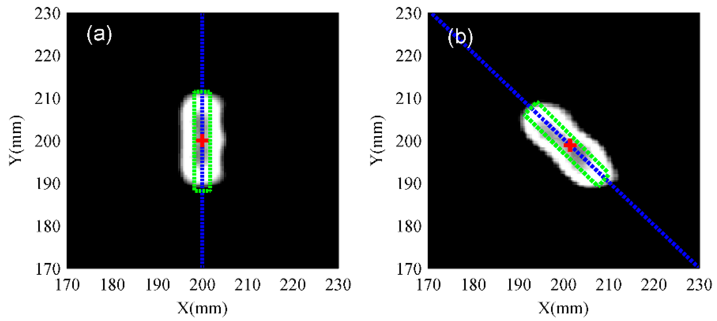
Figure 15.
The direction identification of an inclined rectangular groove based on the numerical result. (a) 90°; (b) 135°. The red plus (+) indicates the centroid location. The blue dashed line is the spindle. The green dash line is the boundary of the inclined rectangular groove. The background image is a grayscale image which is processed by a threshold at the level of −3 dB.

Figure 16.
Schematic of the experimental setup.

Figure 17.
Band-pass filtering of an experimental signal. (a) Original signal; (b) spectrum of the original signal; (c) filtered signal; (d) spectrum of the filtered signal.
Figure 17.
Band-pass filtering of an experimental signal. (a) Original signal; (b) spectrum of the original signal; (c) filtered signal; (d) spectrum of the filtered signal.

Figure 18.
Experimental results of Case 1 to Case 3. (a) Wavenumber distribution of Case 1; (b) depth distribution of Case 1; (c) wavenumber distribution of Case 2; (b) depth distribution of Case 2; (d) wavenumber distribution of Case 3; (e) depth distribution of Case 3. The white circle represents the actual location of the damage. The actual defect depth of Case 1 and Case 3 is 1 mm, while the actual defect depth of Case 2 is 0.5 mm.

Figure 19.
Experimental results of Case 5 and Case 7. (a) Wavenumber distribution of Case 5; (b) depth distribution of Case 5; (c) wavenumber distribution of Case 7; (d) depth distribution of Case 7. The white circle represents the actual location of the damage. The actual depth of the defect is 1 mm.

Figure 20.
Experimental results of Case 8 and Case 9. (a) Wavenumber distribution of Case 8; (b) depth distribution of Case 8; (c) wavenumber distribution of Case 9; (d) depth distribution of Case 9. The white circle represents the actual location of the damage. The actual depth of the defect is 1 mm.

Figure 21.
Experimental results of Case 10 and Case 11. (a) Wavenumber distribution of Case 10; (b) depth distribution of Case 10; (c) wavenumber distribution of Case 11; (d) depth distribution of Case 11. The white rectangle represents the actual location of the damage. The actual depth of the defect is 1 mm.

Figure 22.
The direction identification of an inclined rectangular groove based on the experimental result. (a) 90°; (b) 135°. The red plus (+) indicates the centroid location. The blue dashed line is the spindle. The green dash line is boundary of the inclined rectangular groove. The background image is a grayscale image which is processed by a threshold at the level of −3 dB.

Figure 23.
The wavenumber distributions of the spatial window when different conditions are taken into consideration. (a) Condition 1; (b) condition 2; (c) condition 3; (d) condition 4; (e) condition 5; (f) condition 6. The conditions are listed in Table 9.
Figure 23.
The wavenumber distributions of the spatial window when different conditions are taken into consideration. (a) Condition 1; (b) condition 2; (c) condition 3; (d) condition 4; (e) condition 5; (f) condition 6. The conditions are listed in Table 9.

Figure 24.
The test results obtained under various window radii. (a) 5 mm; (b) 6 mm; (c) 7 mm; (d) 8 mm; (e) 9 mm; (f) 10 mm; (g) 11 mm; (h) 12 mm. The white circle represents the actual location of the damage. The central frequency of the excitation signal is 400 kHz. A circular flat bottom hole is located in (185, 185).

Figure 25.
The maximum wavenumber obtained under various window radii. The central frequency of the excitation signal is 400 kHz.
Figure 25.
The maximum wavenumber obtained under various window radii. The central frequency of the excitation signal is 400 kHz.


Table 1.
Properties of the 6061-T6 aluminum plate.
| Property | Value |
|---|---|
| Density | 2700 (kg/m3) |
| Young’s modulus | 68.9 (GPa) |
| Poissons’ratio | 0.33 |
Table 2.
Specimen parameters.
| Specimen | Damage Type | Excitation Source Position (mm) | Central Position of Damage (mm) | Radius (mm) | Depth (mm) | Inclined Degree (°) | Width (mm) | Length (mm) |
|---|---|---|---|---|---|---|---|---|
| Case 1 | One flat bottom hole | (100, 200) | (200, 200) | 5 | 1 | / | / | / |
| Case 2 | One flat bottom hole | (100, 200) | (200, 200) | 5 | 0.5 | / | / | / |
| Case 3 | One flat bottom hole | (100, 200) | (200, 200) | 3.5 | 1 | / | / | / |
| Case 4 | Two flat bottom holes | (100, 200) | No. 1: (200, 215) | 5 | 1 | / | / | / |
| No. 2: (200, 185) | 5 | 1 | / | / | / | |||
| Case 5 | Two flat bottom holes | (100, 200) | No. 1: (200, 210) | 5 | 1 | / | / | / |
| No. 2: (200, 190) | 5 | 1 | / | / | / | |||
| Case 6 | Two flat bottom holes | (200, 100) | No. 1: (200, 215) | 5 | 1 | / | / | / |
| No. 2: (200, 185) | 5 | 1 | / | / | / | |||
| Case 7 | Two flat bottom holes | (200, 100) | No. 1: (200, 210) | 5 | 1 | / | / | / |
| No. 2: (200, 190) | 5 | 1 | / | / | / | |||
| Case 8 | Two flat bottom holes | (200, 100) | No. 1: (200, 210) | 5 | 1 | / | / | / |
| No. 2: (200, 190) | 3.5 | 1 | / | / | / | |||
| Case 9 | Two flat bottom holes | (200, 100) | No. 1: (200, 210) | 3.5 | 1 | / | / | / |
| No. 2: (200, 190) | 5 | 1 | / | / | / | |||
| Case 10 | One groove | (100, 200) | (200, 200) | / | 1 | 90 | 4 | 24 |
| Case 11 | One groove | (100, 200) | (200, 200) | / | 1 | 135 | 4 | 24 |
Table 3.
The depth evaluations of Case 1 to Case 3.
| Specimen | Actual Depth (mm) | Reconstructed Depth (mm) | Estimation Error of Depth |
|---|---|---|---|
| Case 1 | 1 | 0.9887 | 1.13% |
| Case 2 | 0.5 | 0.4837 | 3.26% |
| Case 3 | 1 | 0.9183 | 8.17% |
Table 4.
The depth evaluations of Case 4 to Case 7.
| Specimen | Actual Depth (mm) | Reconstructed Depth (mm) | Estimation Error of Depth | |
|---|---|---|---|---|
| Case 4 | No. 1 | 1 | 0.9917 | 0.83% |
| No. 2 | 1 | 0.9917 | 0.83% | |
| Case 5 | No. 1 | 1 | 0.9887 | 1.13% |
| No. 2 | 1 | 0.9887 | 1.13% | |
| Case 6 | No. 1 | 1 | 0.9946 | 0.54% |
| No. 2 | 1 | 0.9976 | 0.24% | |
| Case 7 | No. 1 | 1 | 0.9887 | 1.13% |
| No. 2 | 1 | 0.9976 | 0.24% | |
Table 5.
The depth evaluations of Case 8 and Case 9.
| Specimen | Actual Depth (mm) | Reconstructed Depth (mm) | Estimation Error of Depth | |
|---|---|---|---|---|
| Case 8 | No. 1 | 1 | 0.9976 | 0.24% |
| No. 2 | 1 | 0.9183 | 8.17% | |
| Case 9 | No. 1 | 1 | 0.9524 | 4.76% |
| No. 2 | 1 | 0.9917 | 0.83% | |
Table 6.
The depth and angle evaluations of Case 10 and Case 11.
| Specimen | Actual Depth (mm) | Reconstructed Depth (mm) | Estimation Error of Depth | Actual Incidence Angle (°) | Reconstructed Angle (°) | Estimation Error of Angle |
|---|---|---|---|---|---|---|
| Case 10 | 1 | 0.8705 | 12.95% | 90 | 90.00 | 0.00% |
| Case 11 | 1 | 0.8640 | 13.60% | 135 | 134.84 | 0.12% |
Table 7.
The depth evaluations of Case 1 to Case 3, Case 5, Case 7, Case 8, and Case 9.
| Specimen | Actual Depth (mm) | Reconstructed Depth (mm) | Estimation Error of Depth | |
|---|---|---|---|---|
| Case 1 | 1 | 0.9432 | 5.68% | |
| Case 2 | 0.5 | 0.4490 | 10.20% | |
| Case 3 | 1 | 0.8673 | 13.27% | |
| Case 5 | No. 1 | 1 | 0.9308 | 6.92% |
| No. 2 | 1 | 0.9401 | 5.99% | |
| Case 7 | No. 1 | 1 | 0.9152 | 8.48% |
| No. 2 | 1 | 0.9277 | 7.23% | |
| Case 8 | No. 1 | 1 | 0.9339 | 6.61% |
| No. 2 | 1 | 0.8636 | 13.64% | |
| Case 9 | No. 1 | 1 | 0.8866 | 11.34% |
| No. 2 | 1 | 0.9246 | 7.54% | |
Table 8.
The depth and angle evaluations of Case 10 and Case 11.
| Specimen | Actual Depth (mm) | Reconstructed Depth (mm) | Estimation Error of Depth | Actual Incidence Angle (°) | Reconstructed Angle (°) | Estimation Error of Angle |
|---|---|---|---|---|---|---|
| Case 10 | 1 | 0.8510 | 14.90% | 90 | 92.37 | 2.63% |
| Case 11 | 1 | 0.8345 | 16.55% | 135 | 143.46 | 6.27% |
Table 9.
The conditions of Figure 23.
Table 9.
The conditions of Figure 23.
| Condition | Damage Type | Excitation Source Position (mm) | Central Position of Damage (mm) | Damage Radius (mm) | Damage Depth (mm) | Central Position of Spatial Window (mm) | Spatial Window Radius (mm) |
|---|---|---|---|---|---|---|---|
| Condition 1 | One flat bottom hole | (200, 100) | (200, 210) | 5 | 1 | (200, 210) | 8 |
| Condition 2 | One flat bottom hole | (200, 100) | (200, 215) | 5 | 1 | (200, 215) | 8 |
| Condition 3 | One flat bottom hole | (200, 100) | (200, 220) | 5 | 1 | (200, 220) | 8 |
| Condition 4 | Two flat bottom holes | (200, 100) | No. 1: (200, 210) | 5 | 1 | (200, 210) | 8 |
| No. 2: (200, 190) | 5 | 1 | |||||
| Condition 5 | Two flat bottom holes | (200, 100) | No. 1: (200, 215) | 5 | 1 | (200, 215) | 8 |
| No. 2: (200, 185) | 5 | 1 | |||||
| Condition 6 | Two flat bottom holes | (200, 100) | No. 1: (200, 220) | 5 | 1 | (200, 220) | 8 |
| No. 2: (200, 180) | 5 | 1 |
© 2018 by the authors. Licensee MDPI, Basel, Switzerland. This article is an open access article distributed under the terms and conditions of the Creative Commons Attribution (CC BY) license (http://creativecommons.org/licenses/by/4.0/).
Share and Cite
MDPI and ACS Style
Fan, G.; Zhang, H.; Zhang, H.; Zhu, W.; Chai, X. Lamb Wave Local Wavenumber Approach for Characterizing Flat Bottom Defects in an Isotropic Thin Plate. Appl. Sci. 2018, 8, 1600. https://doi.org/10.3390/app8091600
AMA Style
Fan G, Zhang H, Zhang H, Zhu W, Chai X. Lamb Wave Local Wavenumber Approach for Characterizing Flat Bottom Defects in an Isotropic Thin Plate. Applied Sciences. 2018; 8(9):1600. https://doi.org/10.3390/app8091600
Chicago/Turabian StyleFan, Guopeng, Haiyan Zhang, Hui Zhang, Wenfa Zhu, and Xiaodong Chai. 2018. "Lamb Wave Local Wavenumber Approach for Characterizing Flat Bottom Defects in an Isotropic Thin Plate" Applied Sciences 8, no. 9: 1600. https://doi.org/10.3390/app8091600
Note that from the first issue of 2016, this journal uses article numbers instead of page numbers. See further details here.