Ultrasonic Guided Wave-Based Circumferential Scanning of Plates Using a Synthetic Aperture Focusing Technique


1
State Key Laboratory of Fluid Power and Mechatronic Systems, School of Mechanical Engineering, Zhejiang University, 38 Zheda Road, Hangzhou 310027, China
2
Institute of Advanced Digital Technologies and Instrumentation, School of Biomedical Engineering and Instrument Science, Zhejiang University, 38 Zheda Road, Hangzhou 310027, China
*
Author to whom correspondence should be addressed.
Appl. Sci. 2018, 8(8), 1315; https://doi.org/10.3390/app8081315
Submission received: 11 July 2018
/
Revised: 28 July 2018
/
Accepted: 6 August 2018
/
Published: 7 August 2018
(This article belongs to the Special Issue Ultrasonic Guided Waves)
Abstract
:Featured Application
Ultrasonic guided wave scanning of plates with the transducer moving along a circumferential path outside the tested area.
Abstract
Tanks are essential facilities for oil and chemical storage and transportation. As indispensable parts, the tank floors have stringent nondestructive testing requirements owing to their severe operating conditions. In this article, a synthetic aperture focusing technology method is proposed for the circumferential scanning of the tank floor from the edge outside the tank using ultrasonic guided waves. The zeroth shear horizontal (SH0) mode is selected as an ideal candidate for plate inspection, and the magnetostrictive sandwich transducer (MST) is designed and manufactured for the generation and receiving of the SH0 mode. Based on the exploding reflector model (ERM), the relationships between guided wave fields at different radii of polar coordinates are derived in the frequency domain. The defect spot is focused when the sound field is calculated at the radius of the defect. Numerical and experimental validations are performed for the defect inspection in an iron plate. The angular bandwidth of the defect spot is used as an index for the angular resolution. The results of the proposed method show significant improvement compared to those obtained by the B-scan method, and it is found to be superior to the conventional method—named delay and sum (DAS)—in both angular resolution and calculation efficiency.
1. Introduction
Tanks are essential facilities for the storage and transportation of petroleum products. Thousands of tanks may be in service at the same time in one oil depot. Because of the harsh working conditions and corrosive storage materials, various kinds of defects, which are hidden hazards, may occur in the tanks. The structural integrity failure of the tanks may cause catastrophic accidents such as environmental pollution and explosions [1]. Thus, tanks require stringent inspection for their long-term and high-level safety. Tank floors are indispensable parts of the tanks. It is found that 80% of corrosion, which makes up the majority of the defects in the tanks, occur in the tank floors, making them key areas in the overhauls [2]. The most common non-destructive testing technologies for tank floors based on flux leakage [3,4,5] and ultrasonics [6] are limited for the low working efficiency of testing “step by step.” The tanks must stop their service and be emptied before the inspection. The cost and time for the overhaul of the tank floors can amount to hundreds of thousands of dollars and dozens of days. Recently, a technology based on sound emission has been introduced for the structural health monitoring of tanks in service [7,8,9]. Elastic waves caused by the crack growth and liquid leakage are collected and analyzed for the damage detection. However, useful information is difficult to extract from the signals because of the low signal-to-noise ratios, and the localization of the damage is dissatisfactory with a limited number of transducers. Therefore, it is urgent and highly desirable to develop new methods for testing tank floors in service.
Ultrasonic guided wave methods have been proven to have tremendous potential in the rapid inspections of structures with long and slender dimensions such as pipes [10,11], plates [12,13,14], and rails [15]. For the inspection of plate structures such as tank floors, large areas can be inspected at the same time with one transducer using guided waves. Structural health monitoring based on guided waves has been proposed for years. The transducers are permanently installed on the plate around the monitored region. The transducers work as actuators, in turn, and all the others are sensors. The received signals are compared with those acquired when the integrity of the tank floors was confirmed. The coefficients to evaluate the signal changes can be amplitude differences of the direct waves [16] and the variations of the whole signals, named the signal difference coefficient (SDC) [17,18,19,20,21]. Different imaging methods are introduced for guided wave monitoring, such as the filtered back-projection method (FBP) [22], the interpolated FBP (IFBP) [23], the algebraic reconstruction technique (ART) [24], and the probabilistic reconstruction algorithm (PRA) [25], which are all basically drawn from computational tomography (CT). Recently, a method called full waveform inversion (FWI) has been introduced for guided wave monitoring [26,27]. Guided waves with high frequency dispersions are used, and the model of the monitored area is constructed and revised in the frequency domain to match the signals acquired by the model and those collected in the tests. This method performs well in corrosion imaging. However, it should be mentioned that numerous transducers are needed for high sensitivities and localization accuracies in guided wave monitoring, and multiple iterations are required in these methods for high resolutions, which may be time-consuming for large amounts of data.
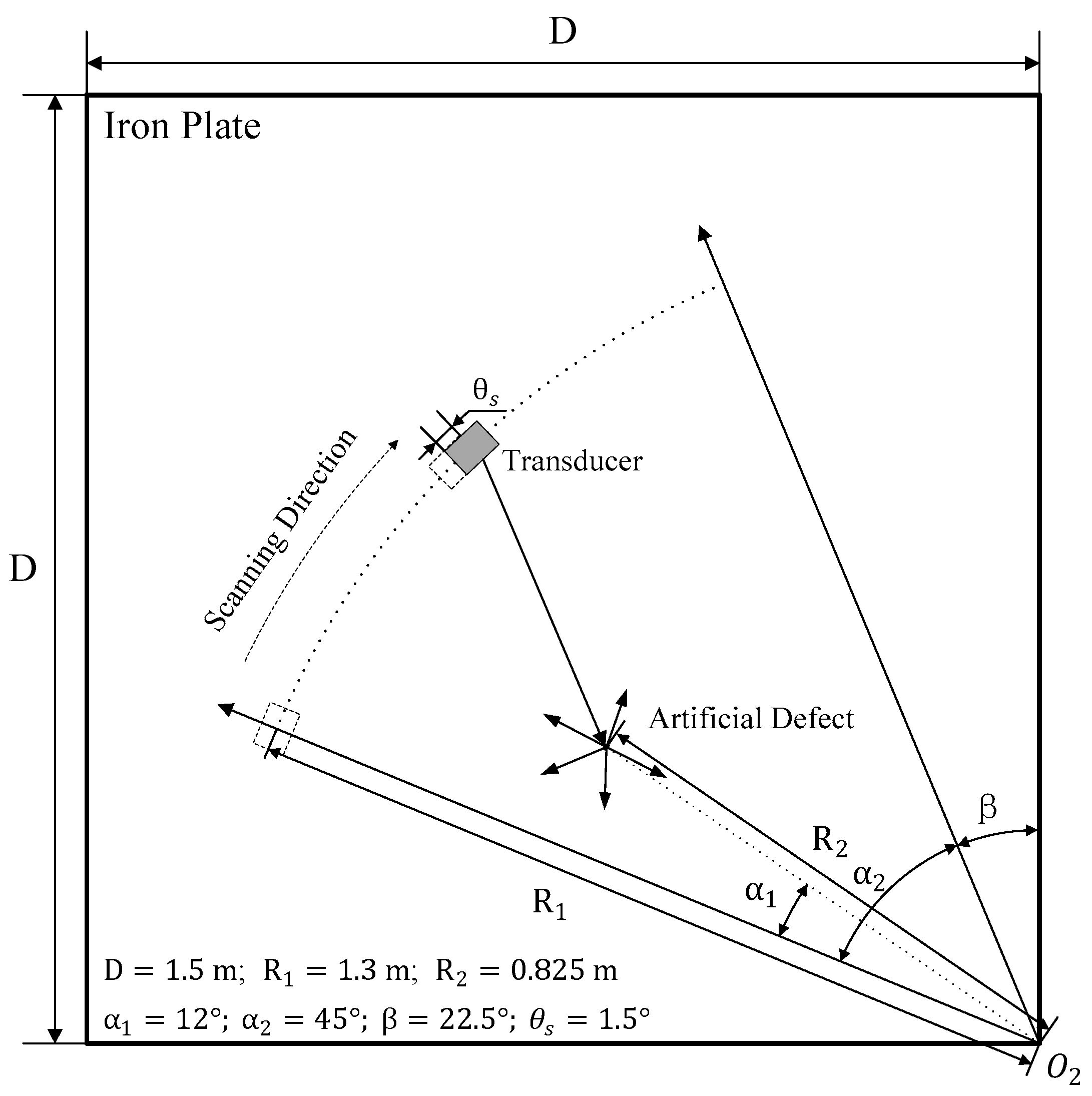
Guided wave scanning is an alternative method for plate inspection. As shown in Figure 1, the tank floor in service can be evaluated with one transducer moving along the edge outside the tank [28]. The spots of the defects in the image of the original signals (i.e., the B-scan image in this study) have long lateral trailing because of the expansion of the sound fields in the plates. To improve the lateral resolution, the synthetic aperture focusing technique (SAFT) is developed. The traditional method of SAFT is called delay and sum (DAS) [29,30]. The wave packets of the defect in different signals can be superposed in the image with the distances between the defect and the transducer locations in the scanning. This method is theoretically applicable for arbitrary scanning paths of the transducer. However, the method is carried out in the time domain with poor computational efficiency, and residual trailing exists in the image. Another method of SAFT is proposed based on sound field migration in the frequency domain, providing better computational efficiency as well as imaging quality compared with the DAS method [31,32,33]. However, the sound field migration of this method is deduced in the Cartesian coordinate system, which can only manage signals acquired by the transducer moving along a straight path. The paths of the transducer for the scanning of the tank floors are circular, making this method inapplicable. Efficient methods of SAFT for guided wave-based circumferential scanning have not been seen yet.
In this paper, a method of SAFT for circumferential scanning (CSAFT) is proposed. In Section 2, the shear horizontal mode in the plates, named SH0, is selected for inspection, and the sound field of the magnetostrictive sandwich transducer (MST) used in this study is calculated; the imaging method is developed based on sound field migration in the polar coordinate systems. In Section 3, the proposed method is verified by numerical simulations and compared with other two methods, the B-scan and DAS methods, for different affecting factors. Experimental verifications are carried out in an iron plate in Section 4 and conclusions follow in Section 5.
2. Method
2.1. Shear Horizontal Waves
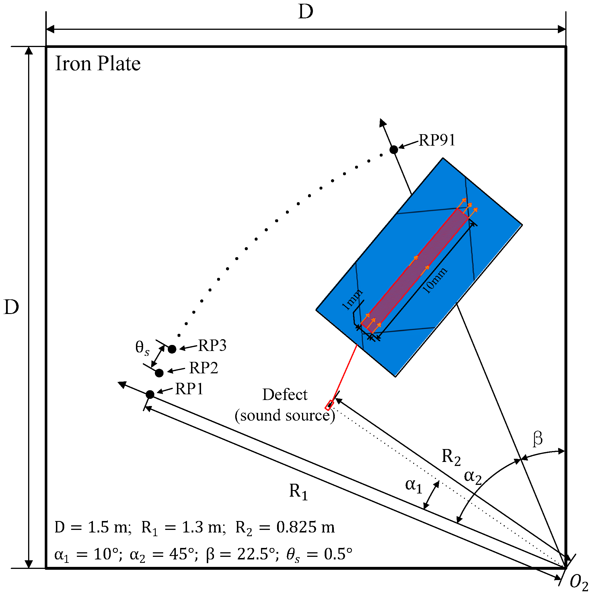
As shown in Figure 1, in circumferential scanning using guided waves, the transducer to generate and receive guided waves moves around the origin point at the radius . The wave front of the incident guided waves expands during the propagation. The reflection waves are generated if the defects are covered by the wave front of the incident waves. The flight time and peak values of the reflection waves are used to evaluate the location and size of the defects, respectively.
Shear horizontal waves (SH waves) and Lamb waves are two kinds of mechanical waves propagating in a solid plate. For waves propagating along the direction as in Figure 1, displacements along the direction occur in Lamb waves, which are perpendicular to the plane of the plate, but the displacements of SH waves are along the direction within the plane of the plate. Considering that the tank floors in service are in contact with liquids (storage materials, such as different kinds of oil) and that the attenuation of shear waves in liquids is much higher than that of longitudinal waves, SH waves may be better candidates for an inspection with less energy leakage. Researches of torsional waves in pipes filled with liquids and bars immersed in liquids can be found in [34,35], respectively, as references. Quantitative comparisons of the SH and Lamb waves will be carried out further under the conditions of different kinds of petroleum products with various volumes. And affecting factors such as the curvatures of the tank floors caused by the gravities of the stored materials and sludge deposition under the tank floors will be investigated as well. The SH waves are hardly affected by liquids [36]. Therefore, in this study, with the purpose of verification of the proposed imaging method, the model is simplified as an isotropic plate with the thickness without contact of liquids, the dispersion equation of SH waves can be expressed as [37]
where ,, , and are frequency, phase velocity, and order, respectively, and is the fundamental shear wave velocity, which is determined by mechanical properties of the plate such as density , Young’s modulus , and Poisson’s ratio . Combining the definition of the wave number , the group velocity , and Equations (1) and (2), dispersion curves of phase velocity and group velocity can be calculated:
where is the frequency-thickness product. Dispersion curves of phase velocity and group velocity for the iron plates with mechanical properties , , and are shown in Figure 2. All the modes are named by their orders, and for the wave mode , a frequency lower limit exists when is no less than 1, which is called the cutoff frequency.
The thickness of the tank floor commonly used is between 6 and 19 mm [38]. In this study, the thickness of the iron plate used for the verification in numerical simulations and experiments is selected as 4 mm for the easy operations in the laboratory. The wave structures of SH0, SH1, SH2, and SH3 modes in the direction are shown in Figure 3. It can be observed that the pure SH0 mode without dispersion can be generated when the excitation frequency is lower than the cutoff frequency of the SH1 mode. Compared with high order modes (SH1, SH2 and SH3), the wave structure of the SH0 mode is uniform along the thickness, giving the same detectability for the defects within the plates and on the surfaces. With these advantages, the SH0 mode is selected for inspection in this study.
2.2. The Sound Field of the Transducer
Piezoelectric and magnetostrictive transducers are commonly used in guided wave generation. Because of the differences in the principles of energy conversion and transducer structures, piezoelectric transducers are good at out-of-plane displacement generation, while magnetostrictive transducers have advantages in in-plane displacement generation. The magnetostrictive effect of the ferromagnetic materials is made use of in the wave generation, and the inverse magnetostrictive effect works in receiving waves. Details of the working principles of this kind of transducer can be found in [39].
The transducer used in this study is named the magnetostrictive sandwich transducer (MST), with a structure shown in Figure 4. The magnetostrictive strip is the main component for energy conversion in both wave generation and receiving, with the residual magnetism along the direction by pre-magnetization. The soft magnet is used to reduce the magnetic resistance of the dynamic magnetic fields, improving energy conversion efficiency. There are two coils in the MST to generate and sense the dynamic magnetic fields. Coil 1 is ahead of Coil 2 in the direction . is the wavelength of the guided wave. The burst signals in Coil 1 and Coil 2 have a phase difference of . Wires in the working region of the MST are distributed with equal intervals and numbered with from 1 to 40. The current direction and initial phase of all the wires are listed in Table 1.
Each wire in the working region can be regarded as a line sound source, and the sound field for the wnth wire can be derived as [40]
where the wave number , is a constant coefficient, and and denote the relative position between the wnth wire and the receiving point as in Figure 4. is half the length of the working region. Equation (6) is valid when . The sound field of the MST can be calculated as the sound field combinations of all wires:
As mentioned in Section 2.1, the thickness of the iron plate used in this study is . The group velocity and phase velocity of the SH0 mode are both , as in Figure 2. The wave length of the SH0 mode is 25.1 mm as the width of the magnetostrictive strip available is 50.2 mm. Thus, the main frequency of the designed MST is 128 kHz, which is below the cutoff frequency of the SH1 mode (401 kHz). It should be noted that, as mentioned above, the main frequency of the transducer should be determined with the consideration of both detection sensitivities and testing ranges in field tests. The normalized sound fields of the MSTs with different lengths are shown in Figure 5. The waves are controlled to propagate in one direction, and the amplitudes of the main lobes in the sound fields are much larger than those of the side lobes. It can also be seen that the widths of the main lobes decrease with the increase in the lengths of the MSTs. The divergence angle , defined as the largest angle at which the amplitudes are no less than half of the largest amplitude, is used to denote the width of the main lobes. The relationship between the divergence angles and the lengths of the MSTs from 2 mm to 150 mm are shown in Figure 6.
2.3. Synthetic Focusing Imaging for Circumferential Scanning
The whole procedure of the inspection with the transducer at one location can be described as follows:
- Step 1:
- The transducer generates guided waves towards the defect;
- Step 2:
- The defect is motivated and generates scattering waves;
- Step 3:
- Parts of the scattering waves are received by the transducer.
When the defect is motivated by the incident pure SH0 waves, other modes may exist in the scatter waves because of the mode conversions. These modes are not dominant and they can hardly be detected by the MST in the experiments. Therefore, the mode conversion is not considered in this study. Because of the reciprocity of the sound field and the constant group velocity of the SH0 mode, Steps 1 and 3 can be described in the same way. The defect can be regarded as a sound source that generates guided waves at time ; then, the guided waves propagate to the transducer. Since the sonic path in this assumption is half of the actual path, the group velocity is taken as half of the actual value to maintain the flight time of the defect, i.e., . The above equivalent model is also called the exploding reflector model (ERM) [41]. As in Figure 1, the guided waves generated by the defect at the radius expand before being received by the transducer moving at the radius . If is equal to , there will be no expansion of the guided waves, which are simply generated from the defect at the time . An optimal lateral resolution can be obtained from the guided wave fields at the radius with the time term . The relationships of the guided wave fields at different radii can be deduced as follows.
In Figure 1, the polar coordinate is constructed without considering the direction along the thickness, in which the displacement of the SH0 mode is uniform. The wave equation in a polar coordinate can be written as [42]:
where is the wave field of the point at time , which can be written in the form of an inverse Fourier transform:
where and are the angular wave number and angular frequency, respectively. is the two-dimensional spectrum of which can be solved by substituting Equations (9) into (8):
where and denote the guided wave propagating away from the original point and towards the original point, respectively. () is the th kind of Hank function of the order is the wave number along the radius.
The guided waves generated by the defect propagate away from the original point to the transducer; thus, the transfer function for the guided wave fields at different radii can be derived as
Equation (12) can be simplified using the Rayleigh–Sommerfeld diffraction formula [43]:
This function is valid if is approximately equal to With a given step , the two-dimensional spectrums of the guided wave fields at the radii can be derived with those collected by the transducer at the radius with Equation (13). The focused image can be obtained with the inverse Fourier transforms of the guided wave fields at different radii.
The main steps of the proposed algorithm are described below:
- Step 1:
- A data matrix is constructed with scanning signals collected by the transducer at the radius as column vectors.
- Step 2:
- The two-dimensional Fourier transform of the data matrix is performed to obtain two-dimensional spectrum .
- Step 3:
- The length and number of the radius step are determined; The imaging range of the radius is between and . The counter is 1.
- Step 4:
- Two-dimensional spectrum at the radius is calculated with Equation (13). Row vector is constructed with the summation of each column of the two-dimensional spectrum.
- Step 5:
- The inverse Fourier transform of Row vector is performed. The result is the row of the image matrix. The counter is increased by one.
- Step 6:
- Steps 4 and 5 are executed repeatedly until is larger than . The image matrix is outputted at last.
The attainable angular resolution can be calculated with the similar derivation as in [41]. If the divergence angle is used to determine the angular coverage of the transducer, the thresholds of the angular wave number are and , thus, the bandwidth of the angular wave number is . Attainable angular resolution can be calculated as follows:
For the SH0 mode at a certain frequency, the wave length is constant, and the attainable angular resolutions are affected by the divergence angles, which are determined by the structures of the transducers.
The proposed method is applicable for the circumferential scanning of isotropic plates with non-dispersive modes. For dispersive modes like the Lamb waves and higher-order SH waves, dispersion compensation can be achieved with the relationships between the group velocities and the angular frequencies from the group velocity curves in the calculations of two-dimensional spectrums using Equation (13). For anisotropic plates, the wave equation in Equation (8) is not suitable, since the wave propagations along different directions are not the same. The proposed method may be not applicable.
The detection ability of the circumferential scanning is determined by multiple reasons such as the excitation frequency and the characteristics of the defects (shapes and sizes). With the increments of the excitation frequencies, the detection sensitivities of the waves increase while the propagation distances decrease. The shapes of the defects affect the mode conversions and propagations of the scattering waves. Details can be found in [44].
3. Numerical Simulation and Verification
3.1. Simulation Setup
For simplification, only Steps 2 and 3 in Section 2.3 are carried out in the simulation. As in Figure 7, the side length of the iron plate is 1.5 m; the thickness and material properties are the same as in Section 2.1. The original point is set in the vertex of the lower right corner; the defect is 0.825 m from with a size of , and the angular position is 10°. The defect is motivated with a tone-burst signal, which is acquired by filtering a sinusoidal signal of multiple cycles with a Hanning window, as in Figure 8. The main frequency is 128 kHz. With the angular step of 0.5°, 91 receiving points are set at the radius 1.3 m, which are marked from RP1 to RP91. The MST is always towards the original point during the signal being received from RP1 to RP91.The sound field of the MST for receiving is the same as that for generation, and so the signals collected at these receiving points are modulated by the sound field of the MST to construct the B-scan image.
3.2. Method Comparison and Factor Analysis
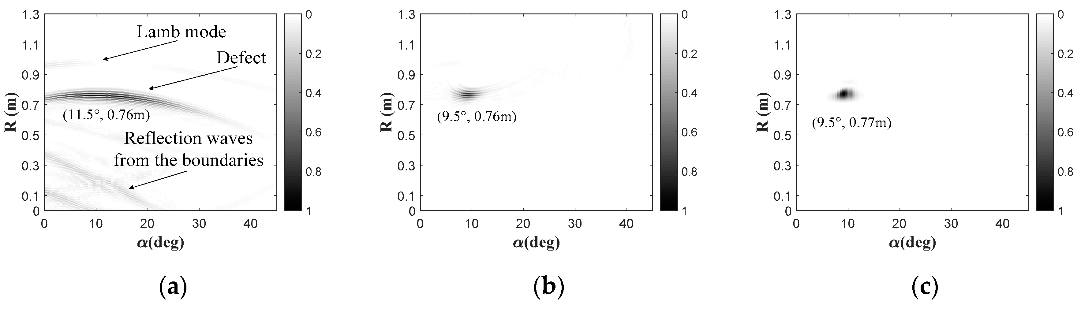
The results of the proposed synthetic aperture focusing technology method for circumferential scanning (CSAFT) are compared with the B-scan image and the results by the DAS method [29]. The sound field of the MST with the length 2L = 70 mm is used to modulate the signals from the simulation. The time signals are turned into distance signals with the group velocity by ; all the distance signals are stacked to become the B-scan image in the order of the angle positions of the receiving points. By the DAS method, the image region is first divided into pixels; then, the flight time of each pixel is calculated with the group velocity and the distance between the pixel and the transducer in the scanning. The amplitude of each pixel is the superposition of the amplitudes extracted from the time signals of the transducer at different positions according to the flight times. It should be noticed that, since only the procedure of receiving is simulated, the group velocity will be the same as the group velocity . The results in Figure 9, Figure 10 and Figure 11 are all calculated with the excitation signal of three cycles.
The results for the angular step are shown in Figure 9. In the B-scan image of Figure 9a, extra waves existing in front of the defect waves are Lamb modes generated by the defect, which travel faster than the SH0 mode. The reflection waves from the boundaries appear after the defect waves. As in Figure 6, the divergence angle of the transducer cannot be zero, and so the defect can also be detected even if it is not directly in front of the transducer. That is the reason for the tailings of the defect waves in the B-scan image, which significantly lower the angular resolution. The image is improved by the DAS method, as in Figure 9b. However, over adjustments exist as a result, leading to some residual trailing. The result of the CSAFT method is shown in Figure 9c. The best angular resolution of the defect spot with the least trailing can be obtained compared with those by other methods. The defect locations (0.76~0.77 m) in Figure 9 are calculated with the peaks of the defect spots, which results in the localization error of the distances (6.7%) for the width of the defect waves in the time signals. The denoted angular positions (9.5~11.5°) have little error compared with the actual value.
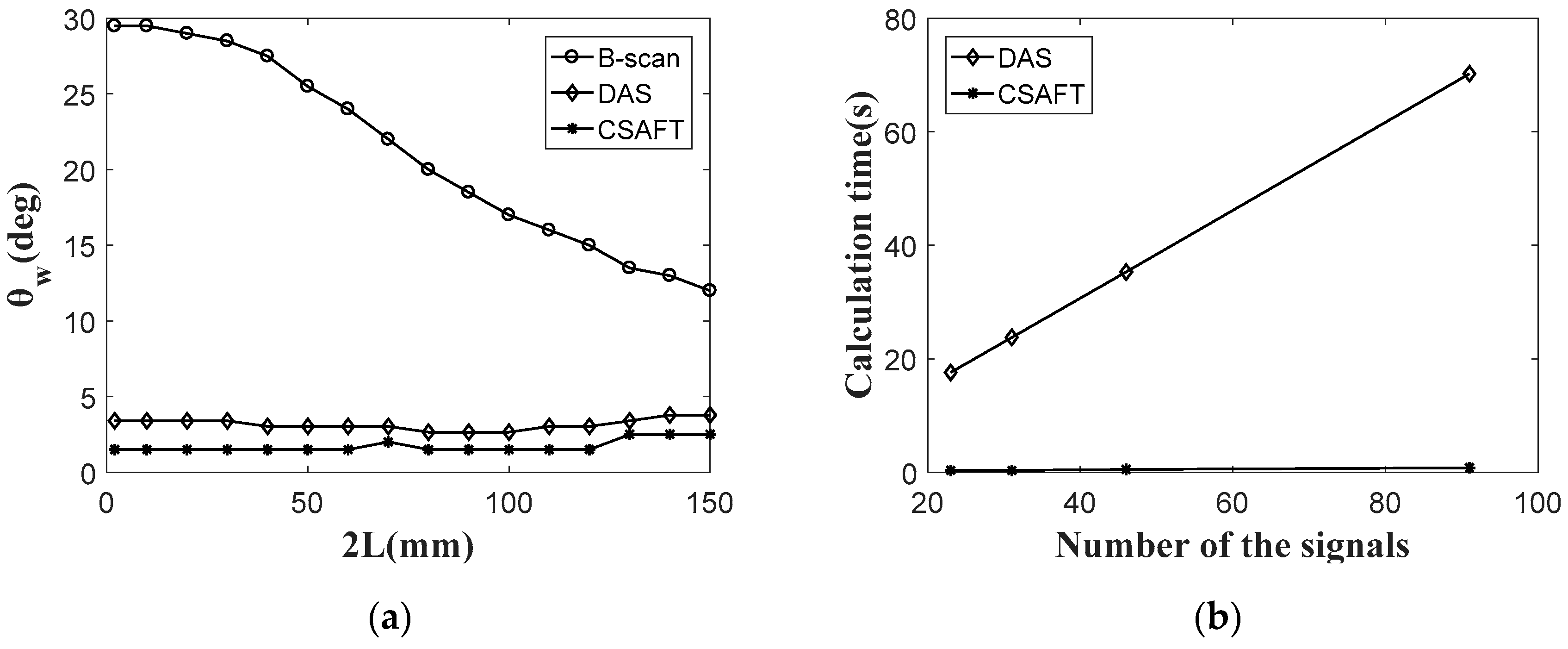
The effect of the length of the transducer is investigated in the simulation. The angular bandwidth of the defect spot , defined as the largest angle range of the region in which the amplitudes are no less than half of the peak, is used to denote the size of the defect spot in the angular direction. The divergence angle of the transducer decreases with the increment of the length of the transducer length 2L as in Figure 6. The angular bandwidth of the defect spot in the B-scan image has the same tendency of decrement as the divergence angle of the transducer, as in Figure 10a, which is 12~29.5° for a length of the transducer between 2 and 150 mm. The DAS method provides a significant improvement of the angular bandwidth (3.4~3.8°), which is basically not affected by the variations of the transducer lengths. The angular bandwidths by the CSAFT method (1.5~2.5°) are slightly superior to those by the DAS method. The CSAFT and DAS method are also compared for different angular steps, which are integral multiples of the minimum angular step . The numbers of the receiving signals for different angular steps are listed in Table 2.
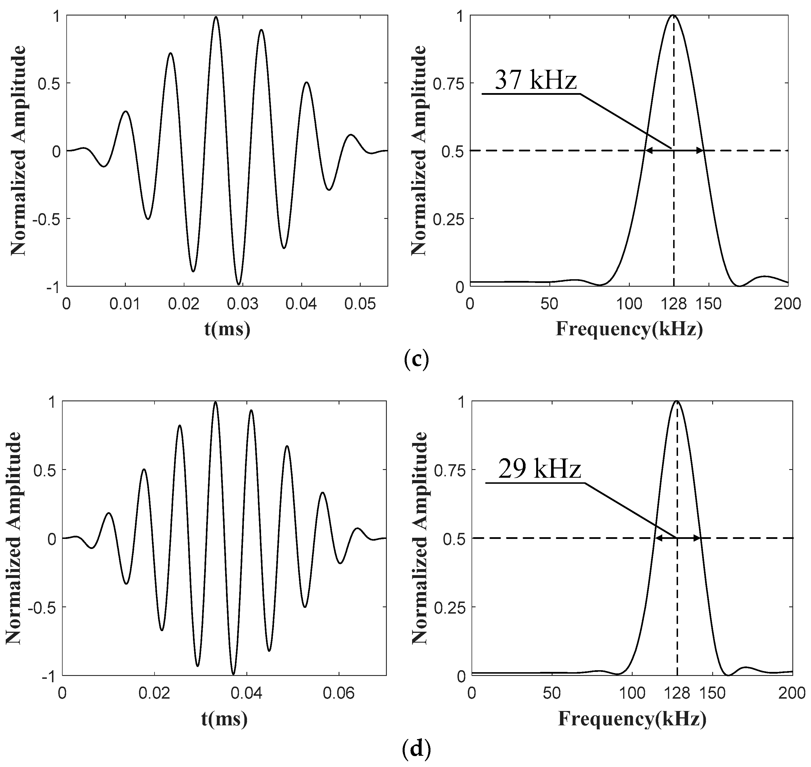
The effect of the excitation signals with different cycles is also studied and the results by the CSAFT method marked with the defect positions and angular bandwidths are shown in Figure 12. It can be observed that the widths of the defects along the radius and the angular bandwidths increase with the increment of the cycles. The defect localization accuracy decreases as well. The increment of the signal cycle is conducive to raising the energy of the incident waves for long testing ranges and narrow down the frequency bandwidth to reduce the influence of other frequencies. However, it extends the lengths of the excitation signals in the time domain, which determine the sizes of the focused defect spots. Both resolutions along the angle and radius are decreased. The cycles of the excitation signals should be selected in the consideration of both resolutions and testing ranges in field tests.
The calculation time of the CSAFT and DAS methods are tested with the same number of the signals in the same computer. As in Figure 10b, the calculation time of the CSAFT method is much less than that of the DAS method, which increases linearly with the numbers of the signals. The advantage of the proposed method in calculation efficiency can be more significant when dealing with a larger amount of data. The images by three methods for different angular steps are presented in Figure 9 and Figure 11. Since the angular sampling rate decreases with the increment of the angular step, the defect spots are coarser in the results of the Bscan and CSAFT method. In the results by the DAS method, over-adjustments get more severe with larger trailing in the image, which may become distractions in defect recognition. The proposed CSAFT method provides the best performance for each angular step.
4. Experimental Investigation
4.1. Experimental Setup
Experiments were carried out to verify the proposed method. As shown in Figure 13, the equipment named the magnetostrictive guided wave detector (MSGW30, Zheda Jingyi Tech, Ltd., Hangzhou, China) was used in the experiments. The equipment has the ability to generate and receive guided waves with the modules including signal generation, power amplification, pre-amplification and A/D conversion under the control of the computer. The coils in the magnetostrictive sandwich transducer (MST) were processed as a flexible printed circuit (FPC), and the material of the magnetostrictive strip is Fe-Co alloy. The circumferential scanning is shown in Figure 14. The iron plate is the same size as that in the simulation. An iron mass scatterer with the additional cross-sectional area of 100 mm2 was coupled on the iron plate at the radius 0.825 m from the original point and 12° from the start position of the scanning as the artificial defect using the epoxy coupling agent. The MST moved around the original point at a radius of 1.3 m with the angular step 1.5° to scan the fan area with an angle of 45°. The MST was used both as an actuator and sensor. The excitation signal used in the experiment is the same as that in the simulation, which is shown in Figure 8a. The sampling ratio is 2 MHz. Thirty-one signals were collected in the scanning. It should be mentioned that the coupling agent used for the coupling between the transducer and the plate is the shear wave coupler (UGW30, Zheda Jingyi Tech, Ltd., Hangzhou, China).
4.2. Results and Discussion
The temperature variations should always be considered in guided wave inspections. The wave velocities are affected by the mechanical properties of the plates, which are changed by the temperature. Wave velocities of collected signals may be different if the scanning is carried out under large temperature variations, affecting the quality of the scanning image. Therefore, wave velocity compensation should be considered. In field tests, the scanning is usually finished within minutes and the temperature does not change rapidly in a short time. However, the situation can be different when the scanning is carried out at a different time (in the day or at night). Thus, wave velocity estimation is necessary before scanning. In this study, the guided waves were generated directly towards one boundary of the plate. The flight time of the reflection waves from the boundary and the distance between the MST and the boundary were used to calculate the group velocity, which is 2714 m/s. The reason for the error (15.4%) of the velocity may be the same as described in Section 3.2, since the peak of the reflection wave was used to determine the flight time.
The results of the three methods are shown in Figure 15. The amplitudes of the images are all normalized between 0 and 1. The estimated peak value of the environmental noise is less than 0.12. The defect spot of the B-scan method in Figure 15a has large trailing, as expected, which may lower the angular resolution. By the DAS method, the trailing around the defect spot is eliminated, as in Figure 15b; however, some trailing occurs in other regions of the image, which have similar amplitudes to the defect spot, becoming a severe distraction in defect recognition. In Figure 15c, the defect spot is improved in the angular direction despite some residual trailing. It can be observed that the defect spot by the DAS method is less obvious than that by the B-scan method, whereas the defect spot by the CSAFT method is much more recognizable. Quantitative comparisons of the defect spot by three methods are listed in Table 3. The position of the defect is denoted by the peak of the spot, and the angular bandwidth is defined as in Section 3.2. The reflection waves from the boundaries are taken as references to show the significance of the defect spots by the three methods. The peak value ratio between the defect and the boundaries by the proposed method is 580% larger than that by the B-scan method, whereas the result with the DAS method does not give any improvement. Apart from the largest significance of the defect, the results by the CSAFT method have the least error in the angular localization and smallest angular bandwidth of the defect compared with the other two methods.
5. Conclusions
A synthetic aperture focusing technique method is proposed for circumferential scanning of plates using guided waves. The SH0 mode is selected for the inspection, which can be effectively generated by the magnetostrictive sandwich transducer (MST). The proposed imaging method is based on the exploding reflector model (ERM) by solving the wave equation in a polar coordinate system and deriving the relationships between guided wave fields at different radii in the frequency domain. Numerical and experimental validation was successfully performed for the circumferential scanning of the defects in an iron plate. The main findings are summarized as follows:
- The SH0 mode has the same detection sensitivity for the cross section of the plate with a uniform wave structure along its thickness; it is nondispersive in frequency and has little energy leakage for the inspection of plates contacted with liquids, which can be generated purely at the frequency below the cutoff frequency of the SH1 mode. The SH0 mode is ideal for the inspection of tank floors in service.
- The MST used for SH0 wave generation can control the wave propagation direction. The main structure of the MST is designed for the SH0 mode at a certain frequency, and the divergence angle can be adjusted with the length of the transducer.
- The angular bandwidth of the defect spot by the proposed method (1.5~2.5°) in the numerical simulations are found to be better than those by the traditional delay and sum (DAS) method (3.4~3.8°) for transducers with different lengths (2~150 mm), both of which have a significant improvement compared with those by the B-scan image (12~29.5°). The proposed method has better calculation efficiency than the DAS method, particularly for a large amount of data. No additional trailing occurs in the image of the proposed method with the increment of the angular step. In circumferential scanning, there should not be too many cycles of the excitation signal when the testing range is sufficient.
- By the proposed method, the peak amplitude of the defect spot can be increased, providing a significant improvement for the defect spot compared with those by the B-scan and DAS methods.
The CSAFT method is expected to be effective for the non-destructive scanning of tank floors in service to minimize the risks and costs of the maintenance operations. For future study, actual oil tank floors installed with accessories will be examined. Defects of different kinds, sizes, and numbers will be inflicted on the tank floor, which will be tested when the oil tank is empty and filled with different kinds of liquids in the field.
Author Contributions
J.W. and S.W. conceived and designed the models and methods presented; Z.T., F.L., and K.Y. helped with the conception and experiments; J.W. performed the simulations, experiments, and data analysis; J.W. and Z.T. wrote this paper.
Funding
The work was supported by the National Natural Science Foundation of China (Grant Nos. 61271084, 51275454, and U1709216) and the Technique Plans of Zhejiang Province (2017C01042).
Conflicts of Interest
The authors declare no conflict of interest.
References
- Tetteh-Wayoe, D. Shell Corrosion Allowance for Aboveground Storage Tanks. In Proceedings of the 2008 7th ASME International Pipeline Conference, Calgary, AB, Canada, 29 September–3 October 2008; American Society of Mechanical Engineers: New York, NY, USA, 2009. [Google Scholar]
- Yang, T.; Zhang, X.; Huang, Z.S.; Yang, F.; Zhang, T.; Wu, J.W. Vertical Tank Bottom Line Integrated Acoustic Defect Detection Technology Research and Application. Pipeline Tech. Equip. 2016, 4, 21–23. (In Chinese) [Google Scholar] [CrossRef]
- Liu, Z.; Kang, Y.; Wu, X.; Yang, S. Study on local magnetization of magnetic flux leakage testing for storage tank floors. Insight 2003, 45, 328–331. [Google Scholar] [CrossRef]
- Ramírez, A.R.; Mason, J.S.; Pearson, N. Experimental study to differentiate between top and bottom defects for MFL tank floor inspections. NDT E Int. 2009, 42, 16–21. [Google Scholar] [CrossRef]
- Usarek, Z.; Warnke, K. Inspection of Gas Pipelines Using Magnetic Flux Leakage Technology. Adv. Mater. Sci. 2017, 17, 37–45. [Google Scholar] [CrossRef] [Green Version]
- Murayama, R.; Makiyama, S.; Kodama, M.; Taniguchi, Y. Development of an ultrasonic inspection robot using an electromagnetic acoustic transducer for a Lamb wave and an SH-plate wave. Ultrasonics 2004, 42, 825–829. [Google Scholar] [CrossRef] [PubMed]
- Kwon, J.R.; Lyu, G.J.; Lee, T.H.; Kim, J.Y. Acoustic emission testing of repaired storage tank. Int. J. Press. Vessel. Pip. 2001, 78, 373–378. [Google Scholar] [CrossRef]
- Riahi, M.; Shamekh, H.; Khosrowzadeh, B. Differentiation of leakage and corrosion signals in acoustic emission testing of aboveground storage tank floors with artificial neural networks. Russ. J. Nondestruct. Test. 2008, 44, 436–441. [Google Scholar] [CrossRef]
- Paulauskiene, T.; Zabukas, V.; Vaitiekūnas, P. Investigation of volatile organic compound (VOC) emission in oil terminal storage tank parks. J. Environ. Eng. Landsc. Manag. 2009, 17, 81–88. [Google Scholar] [CrossRef]
- Zhang, X.W.; Tang, Z.F.; Lv, F.Z.; Pan, X.H. Helical comb magnetostrictive patch transducers for inspecting spiral welded pipes using flexural guided waves. Ultrasonics 2017, 74, 1–10. [Google Scholar] [CrossRef] [PubMed]
- Zhang, X.W.; Tang, Z.F.; Lv, F.Z.; Yang, K.J. Scattering of torsional flexural guided waves from circular holes and crack-like defects in hollow cylinders. NDT E Int. 2017, 89, 56–66. [Google Scholar] [CrossRef]
- Sharma, S.; Mukherjee, A. Ultrasonic guided waves for monitoring corrosion in submerged plates. Struct. Control Health Monit. 2015, 22, 19–35. [Google Scholar] [CrossRef]
- Ostachowicz, W.; Kudela, P.; Malinowski, P.; Wandowski, T. Damage localisation in plate-like structures based on PZT sensors. Mech. Syst. Signal. Proc. 2009, 23, 1805–1829. [Google Scholar] [CrossRef]
- Wilcox, P.D. Omni-directional guided wave transducer arrays for the rapid inspection of large areas of plate structures. IEEE Trans. Ultrason. Ferroelectr. Freq. Control 2003, 50, 699–709. [Google Scholar] [CrossRef] [PubMed]
- Evans, M.; Lucas, A.; Ingram, I. The inspection of level crossing rails using guided waves. Constr. Build. Mater. 2018, 179, 614–618. [Google Scholar] [CrossRef]
- Mazeika, L.; Kazys, R.; Raisutis, R.; Demcenko, A.; Sliteris, R.; Cantore, C. Non-Destructive Testing of Fuel Tanks Using Long-Range Ultrasonic. In Proceedings of the 4th International Conference on Emerging Technologies in Non-Destructive Testing, Stuttgart, Germany, 2–4 April 2007; Busse, G., VanHemelrijck, D., Solodov, I., Anastasopoulos, A., Eds.; Taylor & Francis Ltd.: London, UK, 2011. [Google Scholar]
- Hay, T.R.; Royer, R.L.; Gao, H.D.; Zhao, X.; Rose, J.L. A comparison of embedded sensor Lamb wave ultrasonic tomography approaches for material loss detection. Smart Mater. Struct. 2006, 15, 946. [Google Scholar] [CrossRef]
- Giridhara, G.; Rathod, V.T.; Naik, S.; Mahapatra, D.R.; Gopalakrishnan, S. Rapid localization of damage using a circular sensor array and Lamb wave based triangulation. Mech. Syst. Signal. Proc. 2010, 24, 2929–2946. [Google Scholar] [CrossRef]
- Rathod, V.T.; Mahapatra, D.R. Ultrasonic Lamb wave based monitoring of corrosion type of damage in plate using a circular array of piezoelectric transducers. NDT E Int. 2011, 44, 628–636. [Google Scholar] [CrossRef]
- Chakraborty, N.; Rathod, V.T.; Mahapatra, D.R.; Gopalakrishnan, S. Guided wave based detection of damage in honeycomb core sandwich structures. NDT E Int. 2012, 49, 27–33. [Google Scholar] [CrossRef]
- Ravi, N.B.; Rathod, V.T.; Chakraborty, N.; Mahapatra, D.R.; Sridaran, R.; Boller, C. Modeling Ultrasonic NDE and Guided Wave based Structural Health Monitoring. In Proceedings of the Conference on Structural Health Monitoring and Inspection of Advanced Materials, Aerospace, and Civil Infrastructure, San Diego, CA, USA, 9–12 March 2015; Shull, P.J., Ed.; SPIE—The Internaitional Society for Optical Engineering: Bellingham, WA, USA, 2015. [Google Scholar]
- Zhao, X.; Royer, R.L.; Owens, S.E.; Rose, J.L. Ultrasonic lamb wave tomography in structural health monitoring. Smart Mater. Struct. 2011, 20, 105002. [Google Scholar] [CrossRef]
- Zhao, X.; Rose, J.L. Ultrasonic tomography for density gradient determination and defect analysis. J. Acoust. Soc. Am. 2005, 117, 2546. [Google Scholar] [CrossRef]
- Zhao, X.; Rose, J.L.; Gao, F.D. Determination of density distribution in ferrous powder compacts using ultrasonic tomography. IEEE Trans. Ultrason. Ferroelectr. Freq. Control 2006, 53, 360–369. [Google Scholar] [CrossRef] [PubMed]
- Zhao, X.L.; Gao, H.D.; Zhang, G.F.; Ayhan, B.; Yan, F.; Kwan, C.; Rose, J.L. Active health monitoring of an aircraft wing with embedded piezoelectric sensor/actuator network: I. Defect detection, localization and growth monitoring. Smart Mater. Struct. 2007, 16, 1208–1217. [Google Scholar] [CrossRef]
- Rao, J.; Ratassepp, M.; Fan, Z. Guided wave tomography based on full waveform inversion. IEEE Trans. Ultrason. Ferroelectr. Freq. Control 2016, 63, 737–745. [Google Scholar] [CrossRef] [PubMed]
- Rao, J.; Ratassepp, M.; Fan, Z. Limited-view ultrasonic guided wave tomography using an adaptive regularization method. J. Appl. Phys. 2016, 120, 113–127. [Google Scholar] [CrossRef]
- Puchot, A.R.; Cobb, A.C.; Duffer, C.E.; Light, G.M. Inspection Technique for above Ground Storage Tank Floors using MsS Technology. In Proceedings of the 10th International Conference on Barkhausen and Micro-Magnetics, Baltimore, ML, USA, 21–26 July 2013; Chimenti, D.E., Bond, L.J., Thompson, D.O., Eds.; American Institute Physics: New York, NY, USA, 2014. [Google Scholar]
- Wang, C.H.; Rose, J.T.; Chang, F.K. A synthetic time-reversal imaging method for structural health monitoring. Smart Mater. Struct. 2004, 13, 415–423. [Google Scholar] [CrossRef]
- Pulthasthan, S.; Pota, H.R. Detection, localization and characterization of damage in plates with an, in situ array of spatially distributed ultrasonic sensors. Smart Mater. Struct. 2008, 17, 035035. [Google Scholar] [CrossRef]
- Sicard, R.; Goyette, J.; Zellouf, D. A saft algorithm for lamb wave imaging of isotropic plate-like structures. Ultrasonics 2002, 39, 487–494. [Google Scholar] [CrossRef]
- Sicard, R.; Chahbaz, A.; Goyette, J. Guided lamb waves and l-saft processing technique for enhanced detection and imaging of corrosion defects in plates with small depth-to-wavelength ratio. IEEE Trans. Ultrason. Ferroelectr. Freq. Control 2004, 51, 1287–1297. [Google Scholar] [CrossRef] [PubMed]
- Davies, J.; Cawley, P. The application of synthetic focusing for imaging crack-like defects in pipelines using guided waves. IEEE Trans. Ultrason. Ferroelectr. Freq. Control 2009, 56, 759–771. [Google Scholar] [CrossRef] [PubMed]
- Aristegui, C.; Lowe, M.J.S.; Cawley, P. Guided waves in fluid-filled pipes surrounded by different fluids. Ultrasonics 2001, 39, 367–375. [Google Scholar] [CrossRef]
- Fan, Z.; Lowe, M.J.S.; Castaings, M.; Bacon, C. Torsional waves propagation along a waveguide of arbitrary cross section immersed in a perfect fluid. J. Acoust. Soc. Am. 2008, 124, 2002–2010. [Google Scholar] [CrossRef] [PubMed]
- Kwun, H.; Kim, S.Y.; Light, G.M. Long-range guided wave inspection of structures using the magnetostrictive sensor. J. Korean Soc. NDT 2001, 21, 383–390. [Google Scholar]
- Rose, J.L. Ultrasonic Guided Waves in Solid Media, 1st ed.; Cambridge University Press: Cambridge, UK, 2014; pp. 272–275. ISBN 978-1-107-04895-9. [Google Scholar]
- GB 50341-2014. Code for Design of Vertical Cylindrical Welded Steel Oil Tanks. China National Petroleum Corporation, 2012. Available online: www.csres.com/detail/243638.html (accessed on 29 May 2014).
- Kim, I.K.; Kim, Y.Y. Shear horizontal wave transduction in plates by magnetostrictive gratings. J. Mech. Sci. Technol. 2007, 21, 693–698. [Google Scholar] [CrossRef]
- Lee, J.S.; Kim, Y.Y.; Cho, S.H. Beam-focused shear-horizontal wave generation in a plate by a circular magnetostrictive patch transducer employing a planar solenoid array. Smart Mater. Struct. 2008, 18, 015009. [Google Scholar] [CrossRef]
- Guerra, C.; Biondi, B. Fast 3D migration-velocity analysis by wavefield extrapolation using the prestack exploding-reflector model. Geophysics 2011, 76, WB151–WB167. [Google Scholar] [CrossRef]
- Wu, S.W.; Skjelvareid, M.H.; Yang, K.J.; Chen, J. Synthetic aperture imaging for multilayer cylindrical object using an exterior rotating transducer. Rev. Sci. Instrum. 2015, 86, 083703. [Google Scholar] [CrossRef] [PubMed]
- Haun, M.A.; Jones, D.L.; O’Brien, W.D. Efficient three-dimensional imaging from a small cylindrical aperture. IEEE Trans. Ultrason. Ferroelectr. Freq. Control 2002, 49, 1589–1592. [Google Scholar] [CrossRef]
- Demma, A.; Cawley, P.; Lowe, M. Scattering of the fundamental shear horizontal mode from steps and notches in plates. J. Acoust. Soc. Am. 2003, 113, 1880–1891. [Google Scholar] [CrossRef] [PubMed]
Figure 1.
The diagram of the circumferential scanning using guided waves.

Figure 2.
Dispersion curves of iron plates: (a) phase velocity curves; (b) group velocity curves.

Figure 3.
Wave structures of shear horizontal (SH) modes in the main vibration direction : (a) SH0; (b) SH1; (c) SH2; (d) SH3.
Figure 3.
Wave structures of shear horizontal (SH) modes in the main vibration direction : (a) SH0; (b) SH1; (c) SH2; (d) SH3.


Figure 4.
The structure of the magnetostrictive sandwich transducer (MST).

Figure 5.
The sound fields and divergence angles of the MSTs with different lengths: (a) 2L = 30 mm; (b) 2L = 50 mm; (c) 2L = 70 mm; (d) 2L = 90 mm.
Figure 5.
The sound fields and divergence angles of the MSTs with different lengths: (a) 2L = 30 mm; (b) 2L = 50 mm; (c) 2L = 70 mm; (d) 2L = 90 mm.


Figure 6.
The relationship between the divergence angles of the main lobes and the lengths of the MSTs.
Figure 6.
The relationship between the divergence angles of the main lobes and the lengths of the MSTs.

Figure 7.
The diagram of the numerical model.

Figure 8.
The excitation signals with different cycles and their amplitude spectrums: (a) three cycles; (b) five cycles; (c) seven cycles; (d) nine cycles. The half-decline frequency bandwidth of the signals is marked.
Figure 8.
The excitation signals with different cycles and their amplitude spectrums: (a) three cycles; (b) five cycles; (c) seven cycles; (d) nine cycles. The half-decline frequency bandwidth of the signals is marked.


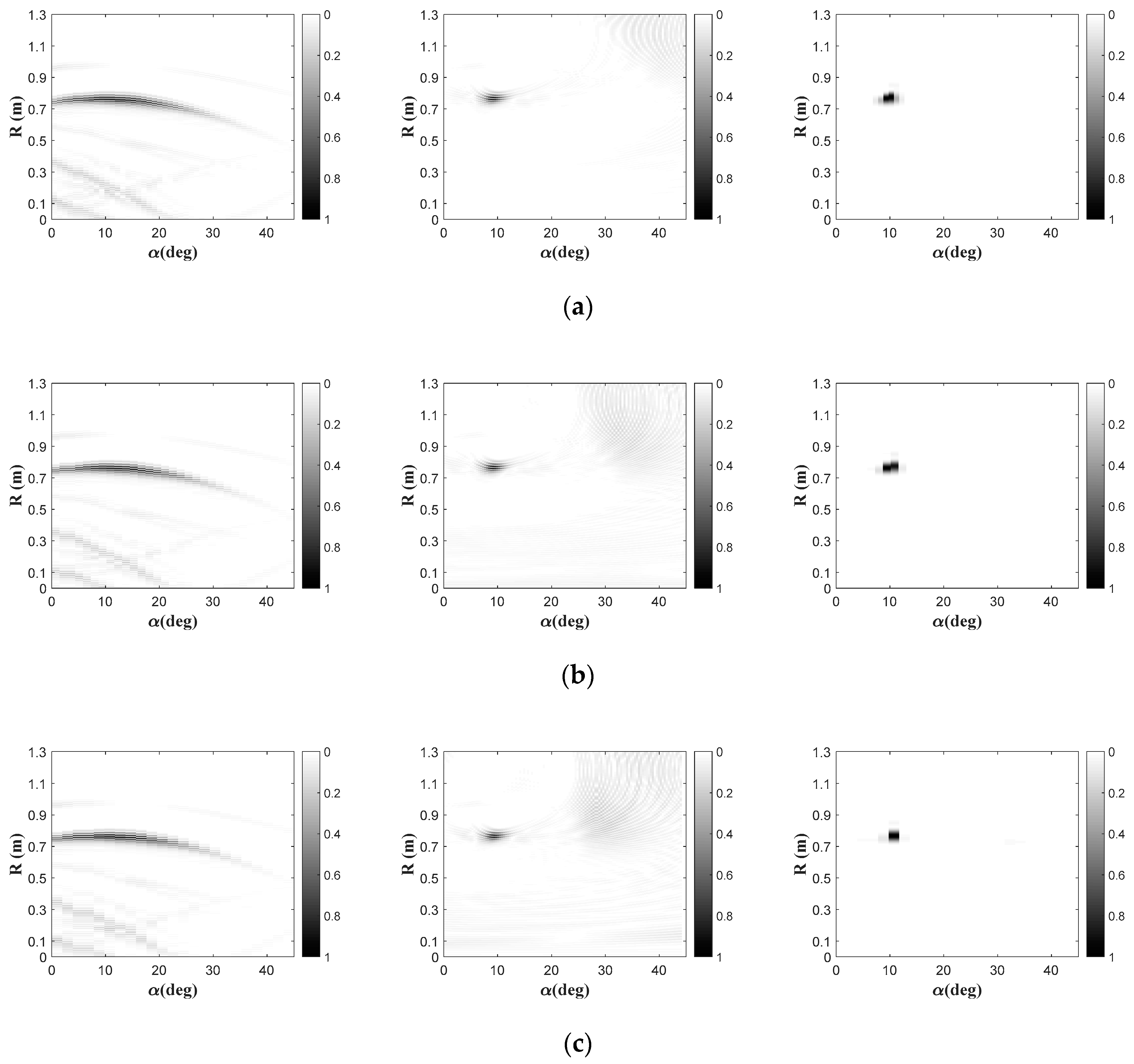
Figure 9.
The results for the angular step by different methods: (a) B-scan, (b) delay and sum (DAS), (c) circumferential synthetic aperture focusing technique (CSAFT). The excitation signal is a tone-burst signal with three cycles.
Figure 9.
The results for the angular step by different methods: (a) B-scan, (b) delay and sum (DAS), (c) circumferential synthetic aperture focusing technique (CSAFT). The excitation signal is a tone-burst signal with three cycles.

Figure 10.
Comparisons of three methods with different factors: (a) the angular bandwidth by the transducer with different lengths; (b) Calculation times with different numbers of signals. The excitation signal is a tone-burst signal with three cycles.
Figure 10.
Comparisons of three methods with different factors: (a) the angular bandwidth by the transducer with different lengths; (b) Calculation times with different numbers of signals. The excitation signal is a tone-burst signal with three cycles.

Figure 11.
Comparisons of the results by the B-scan (Left), DAS (Middle), and CSAFT (Right) methods for different angular steps: (a) ; (b); (c) . The excitation signal is a tone-burst signal with three cycles.
Figure 11.
Comparisons of the results by the B-scan (Left), DAS (Middle), and CSAFT (Right) methods for different angular steps: (a) ; (b); (c) . The excitation signal is a tone-burst signal with three cycles.

Figure 12.
Comparisons of the results by the CSAFT method for excitation signals with different cycles: (a) five cycles; (b) seven cycles; (c) nine cycles. is the angular bandwidth of the defect spot.
Figure 12.
Comparisons of the results by the CSAFT method for excitation signals with different cycles: (a) five cycles; (b) seven cycles; (c) nine cycles. is the angular bandwidth of the defect spot.

Figure 13.
The magnetostrictive guided wave inspection system for circumferential scanning in the plate.
Figure 13.
The magnetostrictive guided wave inspection system for circumferential scanning in the plate.

Figure 14.
Circumferential scanning in the iron plate using guided waves.

Figure 15.
Experimental images by the three methods: (a) B-scan; (b) DAS; (c) CSAFT.


Table 1.
The current direction and initial phase for each wire.
| Name | ||||||||
|---|---|---|---|---|---|---|---|---|
| 1~5 | 6~10 | 11~15 | 16~20 | 21~25 | 26~30 | 31~35 | 36~40 | |
| () | −1 | −1 | 1 | 1 | 22121 | −1 | 1 | 1 |
| () | 0 | 0 | 0 | 0 | ||||
Table 2.
The numbers of the receiving signals for different angular steps.
| Name | Value | |||
|---|---|---|---|---|
| Angular step () | 0.5 | 1 | 1.5 | 2 |
| Number of the signals | 91 | 46 | 31 | 23 |
Table 3.
Defect estimation by the three methods.
| Name | Actual Values | B-Scan | DAS | CSAFT | |
|---|---|---|---|---|---|
| Position | Angle (°) | 12 | 13.5 | 12.5 | 12 |
| Distance (m) | 0.825 | 0.823 | 0.815 | 0.821 | |
| Angular bandwidth (°) | NAN 1 | 4.5 | 3.8 | 2.0 | |
| Peak value ratio (defect/boundaries) | NAN 1 | 0.25 | 0.14 | 1.71 | |
1 NAN means no value for this option.
© 2018 by the authors. Licensee MDPI, Basel, Switzerland. This article is an open access article distributed under the terms and conditions of the Creative Commons Attribution (CC BY) license (http://creativecommons.org/licenses/by/4.0/).
Share and Cite
MDPI and ACS Style
Wu, J.; Tang, Z.; Yang, K.; Wu, S.; Lv, F. Ultrasonic Guided Wave-Based Circumferential Scanning of Plates Using a Synthetic Aperture Focusing Technique. Appl. Sci. 2018, 8, 1315. https://doi.org/10.3390/app8081315
AMA Style
Wu J, Tang Z, Yang K, Wu S, Lv F. Ultrasonic Guided Wave-Based Circumferential Scanning of Plates Using a Synthetic Aperture Focusing Technique. Applied Sciences. 2018; 8(8):1315. https://doi.org/10.3390/app8081315
Chicago/Turabian StyleWu, Jianjun, Zhifeng Tang, Keji Yang, Shiwei Wu, and Fuzai Lv. 2018. "Ultrasonic Guided Wave-Based Circumferential Scanning of Plates Using a Synthetic Aperture Focusing Technique" Applied Sciences 8, no. 8: 1315. https://doi.org/10.3390/app8081315
Note that from the first issue of 2016, this journal uses article numbers instead of page numbers. See further details here.