An Efficient Time Reversal Method for Lamb Wave-Based Baseline-Free Damage Detection in Composite Laminates


1
School of Mechanical Engineering, Xi’an Jiaotong University, Xi’an 710049, China
2
Henan Key Laboratory of Underwater Intelligent Equipment, 713th Research Institute of China Shipbuilding Industry Corporation, Zhengzhou 450015, China
*
Author to whom correspondence should be addressed.
Appl. Sci. 2019, 9(1), 11; https://doi.org/10.3390/app9010011
Submission received: 26 November 2018
/
Revised: 13 December 2018
/
Accepted: 18 December 2018
/
Published: 20 December 2018
(This article belongs to the Special Issue Damage Inspection of Composite Structures)
Abstract
:Featured Application
This paper may develop an efficient and effective damage detection technique to ensure the safety of composite structures.
Abstract
Time reversal (TR) concept is widely used for Lamb wave-based damage detection. However, the time reversal process (TRP) faces the challenge that it requires two actuating-sensing steps and requires the extraction of re-emitted and reconstructed waveforms. In this study, the effects of the two extracted components on the performance of TRP are studied experimentally. The results show that the two time intervals, in which the waveforms are extracted, have great influence on the accuracy of damage detection of the time reversal method (TRM). What is more, it requires a large number of experiments to determine these two time intervals. Therefore, this paper proposed an efficient time reversal method (ETRM). Firstly, a broadband excitation is applied to obtain response at a wide range of frequencies, and ridge reconstruction based on inverse short-time Fourier transform is applied to extract desired mode components from the broadband response. Subsequently, deconvolution is used to extract narrow-band reconstructed signal. In this method, the reconstructed signal can be easily obtained without determining the two time intervals. Besides, the reconstructed signals related to a series of different excitations could be obtained through only one actuating-sensing step. Finally, the effectiveness of the ETRM for damage detection in composite laminates is verified through experiments.
1. Introduction
Composite materials have been widely used in a variety of fields, because of their specific properties, such as its light weight, high stiffness, high strength and corrosion resistance [1,2]. However, due to low velocity impact, manufacturing process and aging, delamination often occurs in the subsurface of material without any obvious indication on the surface. This invisible damage may cause catastrophic failure. Hence, it is required to develop an efficient and effective damage detection technique to ensure the safety of composite structures.
With the advantages of long propagation distance, high sensitivity to different kinds of defects, and low cost, Lamb wave-based damage detection methods have attracted a lot of attention [3,4,5,6,7,8]. However, due to the dispersion characteristic which results in amplitude decrease and wave deformation, Lamb wave signal is always difficult to interpret. Thus most of Lamb wave-based damage detection techniques rely on comparing the test signal with the baseline signal. Since the test signal varies with the environment and boundary conditions, subtle signal changes due to damage may be masked.
To address this issue, researchers have done numerous work regarding baseline-free damage detection in the past decade [9,10]. Specifically, the TRP has been widely used for Lamb wave-based damage detection, as it can not only achieve dispersion self-compensation but also realize baseline-free damage detection in composite laminates [11,12,13,14,15]. In the TRP, an excitation signal is injected in one actuator, the response signal that captured by sensor is then time reversed and re-emitted at the sensor position. Therefore, the frequency components that arrive later will be re-emitted earlier, followed by the components with higher velocities. After the TRP, all the frequency components with different velocities will arrive at the original excitation position concurrently, and thus the dispersion could be compensated. For a healthy structure, the final signal will be the same as the original input signal. In contrast, the two signals will be different from each other if there is any damage present along the propagation path. Therefore, baseline-free damage detection could be realized by comparing the waveform of the reconstructed signal with that of the original input signal.
Researchers have done a lot of work to improve the performance of TRP. Park et al. [13] combined a wavelet-based signal processing technique with TRM to enhance the time-reversibility of Lamb wave in composite laminates. Watkins et al. [16] proposed a modified TRM, which uses a single actuator and multiple sensors. That is, the initial input signal and the secondary excitation signal are actuated by the same actuator. Liu et al. [17] presented a virtual time reversal algorithm which only needs one actuating–receiving step to obtain the reconstructed signal. Agrahari et al. [18] investigated the influences of adhesive layer between the transducer and the host plate, the excitation parameters, the transducer size and the plate thickness on the performance of the TRP to develop an effective damage detection strategy. Xu et al. [19] investigated the effects of single-mode and two-mode Lamb waves on the effectiveness of time reversal damage detection process through theoretical and experimental analysis. And they concluded that, under narrow-band excitation, the time reversibility of single-mode Lamb waves could be greatly improved. Liang et al. [20] and Huang et al. [15] improved the performance of TRM in damage detection through alleviating the influence of the time reversal operator. Agrahari et al. [21] and Mustapha et al. [22] proposed some different damage indices to improve the sensitivity of the TRM to damage. These studies are all aimed at improving the performance of TRP. However, it is still unavoidable that a large number of experiments are required to optimize excitation parameters, and to determine the time intervals in which the waveform of the reconstructed signal is compared with that of the original input signal.
This study comprehensively discussed the effects of the two time intervals on the performance of Lamb wave TRP in composite laminates. Then, an efficient time reversal method (ETRM) is established, which could obtain multiple reconstructed signals related to different excitations through only one actuating-sensing step without determining time intervals. Firstly, a broadband excitation signal is used to acquire Lamb wave responses for a wide range of frequencies. Secondly, the short-time Fourier transform (STFT) combined with a time-varying filter is employed to extract the desired mode components in the time-frequency domain. Then the time-domain waveform of the extracted components is obtained through inverse STFT transform. After that, frequency domain deconvolution is applied to calculate multiple narrow-band reconstructed signals.
The rest of this paper is organized as follows. In Section 2, the theory of the TRM for damage detection is introduced. Then the detailed steps of the proposed efficient time reversal method are given in Section 3. In Section 4, the effectiveness of the ETRM is demonstrated by experiments. The application of the ETRM for damage location in composite laminates is illustrated in Section 5. Finally, conclusions are drawn in Section 6.
2. Baseline-Free Damage Detection Using the Time Reversal Method of Lamb Wave
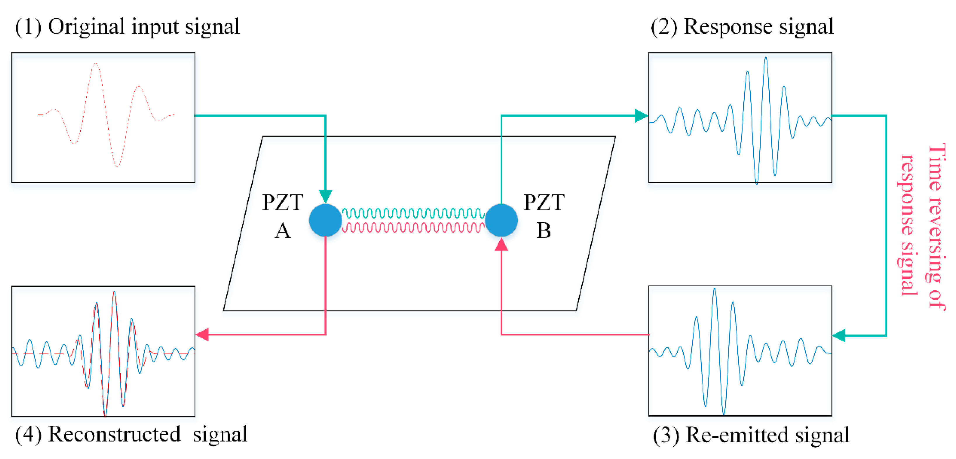
The time reversal method originated from time reversal acoustics [23,24]. Then the time reversal concept extended to Lamb wave propagation to reduce the effects of dispersion and to realize baseline-free damage detection [12,13]. In accordance with the time reversal concept, an original input signal, s(t), can be reconstructed at the initial excitation position A, if the response signal received at position B is reversed in the time domain, and re-emitted from position B to position A. This process is referred to as the time reversibility of Lamb waves. Therefore, damages (e.g., fiber breakage and delamination, crack opening-and-closing) could be detected by comparing the waveform of the reconstructed signal with that of the original input signal [13]. The schematic diagram of the TRP is shown in Figure 1.
The theoretical analysis of the TRP in the frequency domain is described as follows.
Use piezoelectric (PZT) as transducer. When a voltage signal VA(ω) is excited at actuator PZT A, it then converts to mechanical strain εA(ω) and activates a Lamb wave signal that propagates within the plate [25].
where, ω is the angular frequency, and ka(ω) is the electro-mechanical coupling coefficient at PZT A. The response signal, VB(ω,r), that captured by sensor PZT B satisfies,
where, kb(ω) is the electro-mechanical coupling coefficient of PZT B, r is the propagation distance of Lamb waves from actuator to sensor, G(ω,r) is the transfer function of the sensing path. If the actuator and sensor are the same, ka(ω) = kb(ω) [16]. Thus, Equation (2) can be rewritten as,
The response signal inversed in the time domain is equivalent to take complex conjugate in the frequency domain. Thus, the time reverse operation of the response signal VB(ω,r) represented in the frequency domain is,
where, the superscript ‘*’ represents the complex conjugate operation.
The reversed signal is then re-emitted at PZT B which now acts as an actuator. The corresponding response signal captured by PZT A is the reconstructed signal VR(ω,r). It is defined as,
Substituting Equation (4) into Equation (5), the reconstructed signal is rewritten as
Here, |G(ω,r)|2 is referred to as time reversal operator. It varies with frequency because the transfer function G(ω,r) of Lamb waves propagating in composite laminates (including the effects of material damping) is frequency dependent. Therefore, the wave components at different frequencies will be non-uniformly attenuated and the initial input signal cannot be properly reconstructed. To alleviate this problem, narrowband signals are usually used as excitations [13,19].
The TRM-based damage detection is accomplished by comparing the waveform of the reconstructed signal with that of the original input signal. A damage index (DI) is used to measure the discrepancy between the waveform of the original input signal and that of the reconstructed signal. It is defined as follows [14],
where, t0 and t1 define the time interval in which the two waveforms are compared, VA(t) is the original input signal, Vr(t) is the reconstructed signal. The DI value falls within the range of (0, 1). If the two waveforms are fully coincident with each other, DI = 0. If these two waveforms gradually deviate from each other, the DI value increases and approaches 1.
It is noted that when Lamb waves propagate in composite laminates, a response signal consists of many wave components. Such as, wave components propagate through the direct path (from actuator to sensor) and those reflected off from the edges of laminates. Because Lamb wave is easily affected by the boundary conditions, the extracted re-emitted and reconstructed components corresponding only to the direct path. Therefore, the determination of the two time intervals, in which the re-emitted and reconstructed components are extracted respectively, are very difficult. If the time intervals are too narrow, the direct wave components are incomplete. If they are too long, the extracted signal will contain other mode components and noises. Both will result in a large DI value, creating a false alarm of damage.
Moreover, the selection of the excitation parameters is also very important. In order to alleviate the influence of the time reversal operator and improve the SNR, narrowband signal is usually used as the original input signal. However, the time duration of narrowband signal is large. This will lead to the superposition of components in the response signal and reconstructed signal, and then produce a large DI value.
In a word, the traditional TRP requires a large number of experiments to optimize the two time intervals and the excitation parameters, and further each experiment includes two actuating–receiving steps, which can make the experiments time-consuming.
3. An Efficient Time Reversal Method
In this section, an ETRM is proposed to improve the practical applicability and efficiency of the time reversal concept. In the ETRM, multiple reconstructed signals related to different excitations can be acquired through only one actuating-sensing step, and further, the determining of the two time intervals could be avoided. That significantly reduces the hardware manipulation. Figure 2 gives its schematic diagram. The steps of the ETRM are as follows:
(1) A broadband excitation signal is actuated from PZT A, and the response is captured by PZT B;
(2) Time-frequency analysis is performed on the broadband response signal. Then the ridge and the neighbor of the desired components are determined;
(3) Reconstructing the desired components in the time-frequency domain into waveforms in the time domain;
(4) The reconstructed signals related to narrowband excitations are obtained through deconvolution in frequency domain.
The analysis of the ETRM is also given in the frequency domain. As shown in Figure 2, a broadband excitation signal VA(ω) is injected in actuator PZT A. The broadband response signal, VB(ω,r), is captured by sensor PZT B.
Because of dispersion, attenuation and multi-modal propagation, broadband Lamb waves in composite laminates are difficult to interpret. Time-frequency representation (TFR) is an efficient method for the analysis of Lamb wave signal, because it provides a clear illustration for the temporal variation modal energy stream in the time-frequency domain. There are a variety of TFR algorithms that could map the Lamb wave signal from the time domain into time-frequency domain, e.g., short time Fourier transform [26], wavelet transform [27,28], warped frequency transform [29,30], and fractional Fourier transform [31]. Even though some of them cannot to extract and reconstruct the wave components, the time-varying filtering could be employed for breaking this limitation [32,33]. In this paper, for simplicity, the short-time Fourier transform (STFT) is used for illustration.
Mathematically, the STFT of a signal s(t) is formulated as
where, t and ω are the time and angular frequency, respectively, h(τ − t) is a window function (commonly a Hanning or Gaussian window centered at t).
STFT is actually frequency transform of signal pieces in the window. Therefore, the energy of an instantaneous component will spread on the time-frequency plane due to the influence of window. To extract the desired components, not only the points on the ridge but also the adjacent area of the ridge need to be reconstructed. The adjacent area influences the accuracy of mode extraction obviously. A small neighbor area will result in loss of energy, while a large neighbor area may arise noises in the extracted signal.
In this paper, the left and right boundaries are determined by the decibels of the instantaneous frequency energy drop on the ridge. The percentage of energy drop is represented by weight. Figure 2 shows the schematic diagram of mode extraction, where the red solid line is the ridge of a Lamb wave mode. AR is the amplitude of the ridge element corresponding to time t and instantaneous frequency f in the time-frequency matrix. tl and tr are the time range where the magnitude of elements at instantaneous frequency f are larger than weight times AR, i.e.,
Once the left and right boundaries of the neighbor area (the blue area in Figure 3) are determined, the desired components, vd(t,r), could be extracted from the response signal by inverse STFT transform.
Subsequently, the transfer function of the desired Lamb wave mode propagating in the structure, Gd(ω,r), is calculated as follows [34]:
where Vd(ω,r) is the Fourier transform of vd(t,r).
For a narrowband excitation signal Vn(ω), whose bandwidth falls in that of Gd(ω,r), the corresponding response signal Rn(ω,r) can be expressed as follows [34],
Substituting Equation (10) into Equation (11), the narrowband response Rn(ω,r) is obtained as,
It means that the narrowband response could be directly calculated, without requiring hardware operation.
The response signal is then reversed in the time domain. Similar to Equation (4), that could be achieved by taking complex conjugate of the signal in the frequency domain. Next, the time-reversed signal, R*n(ω,r), which acts as a secondary excitation signal, is virtually reemitted back to the structure through PZT B. By taking advantage of the properties of the Green’s functions, it can be easily shown that the elastic response of medium when launching the same excitation function from position A and recording in position B is the same as the one captured at A when launching at B, with no dependence on the geometry of the sample [35]. Hence, the reconstructed signal Rnr(ω,r) received by PZT A could be estimated as,
Substituting Equation (10) into Equation (13), the reconstructed signal could be rewritten as,
The ETRM has following advantages. Firstly, multiple narrow-band reconstructed signals can be obtained through only one broadband actuating-sensing step. Secondly, the response signal and the reconstructed signal only contain a direct wave of a Lamb wave mode. Therefore, there is no need to determine the two time intervals for extracting the re-emitted components and the reconstructed components. Thirdly, the narrow-band extraction process is also a filtering process, which will improve the SNR of the reconstructed signal. In a word, the proposed technique improves the efficiency and accuracy of the TRM.
4. Experiment Investigation
In this section, experiments are designed to investigate the performance of the traditional TRM and the ETRM. The overall test setup consists of an Agilent 33220A function/arbitrary waveform generator (Agilent Technologies, Santa Clara, CA, USA), a NF HSA4012 voltage amplifier (NF corporation, Yokohama, Japan) and a NI PXIe-1082 data acquisition (National Instruments Corporation, NI, North Mopac Expressway Austin, Texas, USA). Two circular PZTs (P-51) with a diameter of 8 mm and a thickness of 0.5 mm are mounted on the surface of the specimen, as shown in Figure 4. The specimen is a T300/7901 16-layer quasi-isotropic carbon fiber-reinforced polymer laminates with the stacked sequence [+45/−45/0/90]2s lay-up. Each laminate is 0.125 mm in thick and the dimensions of the specimen are 690 mm × 690 mm × 2 mm. The material properties of the composite specimen are listed in Table 1.
4.1. The Traditional TRM
In the traditional TRM, transducers change their roles from actuator to sensor and vice versa to reverse the path direction. All the signals in this experiment are measured 128 times at each receiver position to improve the signal-to-noise ratio (SNR).
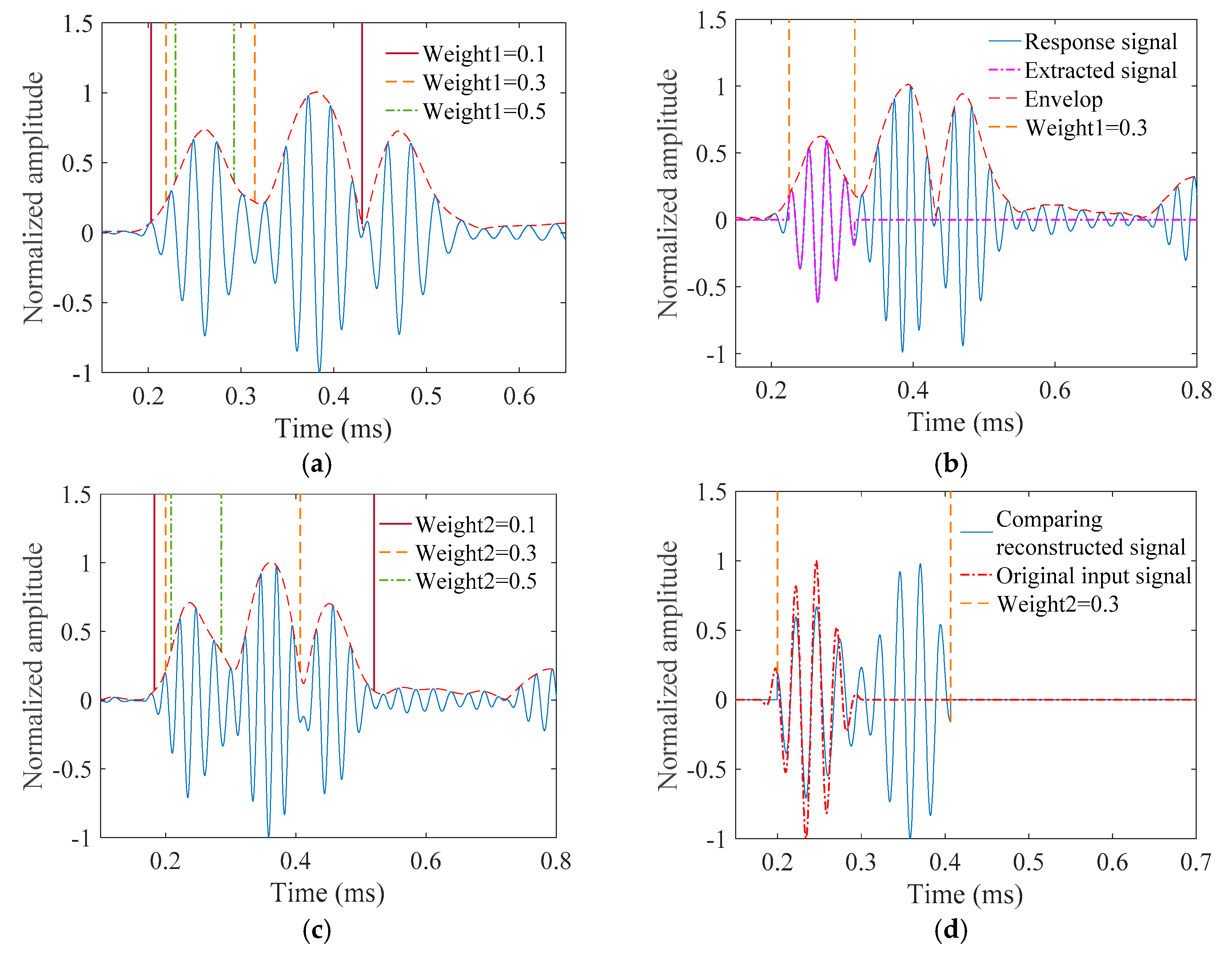
A five-cycle 40-kHz tone burst signal is launched from PZT A. The response signal captured by PZT B is shown in Figure 5a. As mentioned in Section 2, the re-emitted components are extracted from that response signal. To minimize false warning of damage, only the A0 mode components travelling along the direct path between PZT A and PZT B are extracted. In this case, the time interval [t01, t02], in which the components are extracted and time inversed, is a key parameter. Let weight1 to represent the amplitude drop of envelope of the A0 direct wave. The time interval is the time range where the magnitude of direct wave are larger than weight1 times the peak value. As Figure 5a shows, when weight1 = 0.1, components in the time interval (the red solid line) contains both the direct wave and reflected wave. In contrast, when weight1 = 0.3 and 0.5 (the yellow dashed line and the green dash-dotted line), the extracted components only contain the direct wave, however, the direct wave components are incomplete.
Take weight1 = 0.3 as an example; the extracted component is displayed in Figure 5b as the purple dashed-dot line. Then the extracted components are time reversed and re-emitted by PZT B. Following this, the reconstructed signal captured by PZT A is shown in Figure 5c. Take weight2 to represent amplitude drop of envelope of the reconstructed signal. The vertical lines in Figure 5c indicate the ranges at different weight2 values, in which the reconstructed components are compared with the original input signal. For illustration, Figure 5d displays the extracted reconstructed signal when weight2 = 0.3 by the blue solid line. It can be seen that the extracted signal consists of two wave packets, which is quite different from the original input signal (the red dashed-dot line).
Subsequently, the effects of the two time intervals on the accuracy of damage detection are studied. An added mass (20 mm × 20mm × 4mm), is bonded to the specimen as a simulated delamination damage [3,36]. With a fixed weight2 value (i.e., weight2 = 0.4), the evolution of DI values with the variation of weight1 values under healthy and damaged conditions are shown in Figure 6a. It can be seen that, when weigth1 = 0.1 and 0.2, the DI values of healthy condition are even larger than that of the damaged condition. Consequently, it indicates a false warning of damage. What is more, at other weigth1 values, the DI values in healthy and damaged conditions are not significantly different. This will restrict its ability to determine the presence of damage. Figure 5b shows the results, where weight1 is fixed while weight2 changes. It can be seen that weight2 also has a great influence on the DI value.
In practical applications, the determination of weigth1 and weigth2 is related to the physical information and boundary conditions. Thus, it may be time consuming. For example, in this study, six actuating and sensing processes are performed on only one path. Actually, there are dozens of sensing paths for damage detection, which may require hundreds of experiments.
4.2. The ETRM
In this experiment, a typical broadband chirp signal is emitted at PZT A. The equation for the excitation signal is,
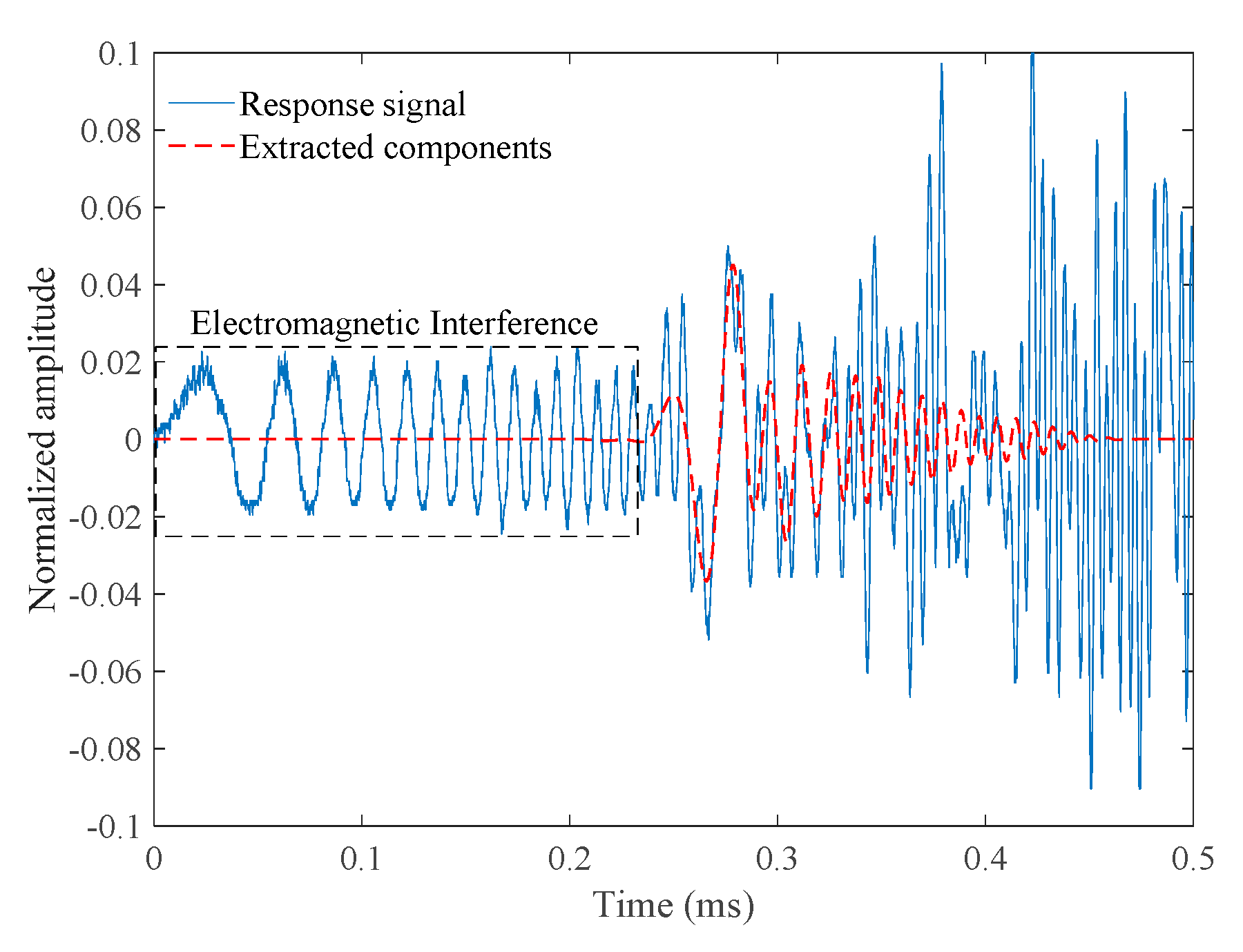
where, f0 is the starting frequency, B is the chirp bandwidth and T is the duration of the chirp signal. Here, f0 takes 10 kHz, B = 600 kHz–10 kHz = 590 kHz, and T takes 1ms. Figure 7 gives the response signal received at PZT B as the blue solid line.
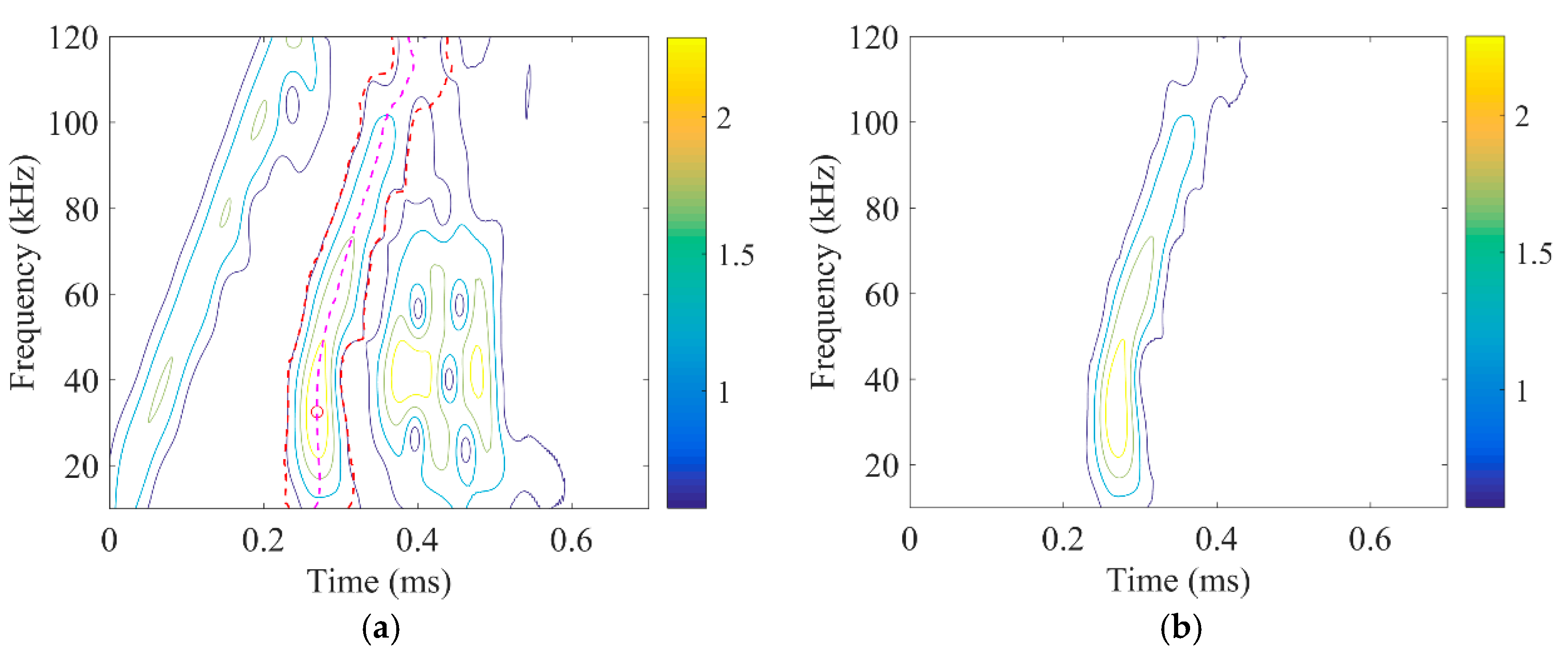
STFT, where the window function takes a Gaussian function with time duration of 0.07 ms, is applied to map the response signal into the time-frequency domain. The STFT spectrogram is shown in Figure 8a. To extract the direct wave components of A0 mode from the response signal, the spectrogram outside the two red dashed lines (as weight takes 0.2) is set to zero (Figure 8b), and then the inverse STFT is applied to reconstruct the residual signal. The time domain waveform of the reconstruct direct wave of A0 mode is shown in Figure 7 as the dotted red line.
Subsequently, the reconstructed signals related to different narrowband excitations could be calculated using Equation (14). For instance, Figure 9a shows the calculated reconstructed signals with different excitation parameters, i.e., five-cycle toneburst, with central frequencies of 40 kHz, 50 kHz, 60 kHz and 70 kHz, respectively. Figure 9b displays the calculated reconstructed signals with a 40 kHz toneburst excitation with cycle numbers 3, 5, 7 and 9, respectively. These demonstrate that the ETRM has the merit of high efficiency.
Furthermore, to investigate the influence of weight value on the performance of damage detection, different weight values (0.1, 0.2, 0.3, 0.4 and 0.5) are used for time-frequency filtering. To ensure consistency, narrow-band excitation with the same parameters as in Section 5 is used in this experiment. Figure 10 gives the DI values with the increase of weight. It can be seen that though the DI values vary with the weight, their values at damaged case keep above the ones at healthy condition. Besides, the relative deviation of DI values in the health and damage conditions at different weight values (i.e., 0.1, 0.2, 0.3, 0.4 and 0.5) are 68.87%, 73.68%, 75.72%, 65% and 76.12%, respectively. It means that the weight value has less influence on the result of damage detection.
5. The Application of ETRM for Damage Imaging of Composite Laminates
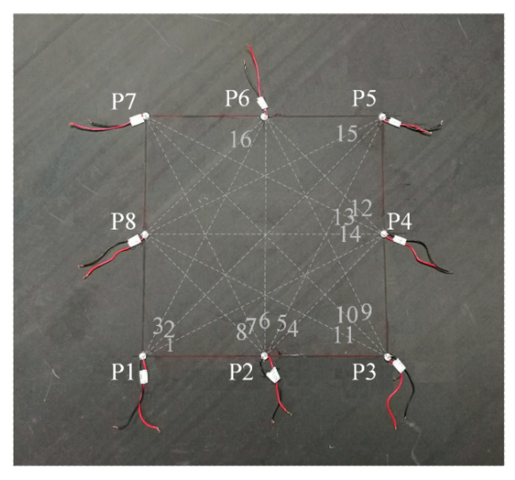
The specimen, PZT and the experiment setup are the same as in Section 4. Eight circular PZTs, with a distance of 140 mm between elements, are bounded on the specimen, and the layout is shown in Figure 11. The dimension of the inspected area is 280 mm × 280 mm. An added mass, with dimension of 30 mm × 20 mm × 5 mm and centering at (46,−46) mm, is placed on the specimen to simulate delamination damage. A coordinate system is established with the origin set at the center of the sensor array. The coordinates of the eight PZTs are shown in Table 2.
In the active sensor array, the eight PZTs take turns as actuator while the rest of them are listening. As shown in Figure 11, there are 16 paths available for damage imaging. A typical chirp signal with frequency sweep from 10 kHz to 600 kHz over a 1-ms window is excited in turn.
The mode extraction method proposed in Section 4 is used to extract the direct wave components of A0 mode. Then the ETRM is used to calculate the narrow-band reconstructed signal corresponding to a five-cycle 40-kHz tone burst excitation. For instance, the comparison between the reconstructed signals and the original input signal of Path 1 and Path 2 is shown in Figure 12a. With damage on the Path 1, the associated reconstructed signal significantly deviate from the original input signal. While, they are almost the same for the healthy Path 2. The DI values of all the 16 paths are shown in Figure 12b. It can be seen that the DI values of Path 1, Path 5 and Path 10 are significantly higher than those of other paths, indicating the presence of damage on these paths.
Subsequently, a probabilistic imaging algorithm is introduced to estimate the location of damage [37,38]. In this algorithm, DI value is used to represent the severity of damage along a sensing path. The inspection area that enclosed in the sensor array is meshed into uniform grids. The probability of damage present at a certain node Ni (i=1, …, n × n) in the inspection area, is defined as,
where, DIj is the DI value of the j-th sensing path, and f(zij) is the Gaussian distribution function defined as follows [39,40],
where, σ is the standard variance, zij indicates the distance from node Ni to the j-th sensing path, it is defined as,
where, (xjA, yjA) and (xjS, yjS) are the coordinates of actuator and sensor of the j-th sensing path, respectively, (xNi, yNi) is the coordinate of node Ni.
Figure 13a–c show the imaging results (i.e., σ = 0.01) as the weight takes 0.1, 0.2 and 0.3, respectively. Each individual image is normalized by its maximum values. The actual center of the simulated damage is indicated by a red ‘o’, and the estimated center is denoted by a blue ‘+’. As Figure 13 shows, the damage location can be accurately located under different weight values. These results demonstrate the effectiveness of the ETRM for damage detection in composite laminates.
For comparison, Figure 14 a, b and c give the imaging results of the traditional TRM as weight1 takes 0.1, 0.2, and 0.3, respectively. It can be seen that the grid with the highest probability value for the presence of damage sits at the sensor sites, rather than the actual damage site. Besides, there are a number of fake peaks at the intersections of different sensing paths, which contaminate the imaging results. It may be possible to obtain accurate results by continuously adjusting the excitation parameters, the weight1 value and weight2 value. But that requires a large number of experiments, i.e., 2 × n × m × p × k experiments, where n indicates the number of propagation paths in the sensor array, m, p, and k represent the number of changes of excitation parameters, weight1 and weight2, respectively. For example, we have conducted 2 × 16 × 1 × 3 × 1 = 96 experiments to obtain these results (Figure 14), which is very time consuming.
6. Conclusions
In this study, the performance of the traditional TRM is discussed theoretically and experimentally. An efficient time reversal technique is further proposed and its effectiveness is verified by experiments.
The traditional TRM requires two actuating–receiving steps for each signal path. Furthermore, it requires determination of the two time intervals, in which the re-emitted components and reconstructed components are extracted. Experimental results showed that these two time intervals have great influence on the performance of TRM. However, the determination of these two time intervals requires a large number of experiments. Thus, it is quite time-consuming.
In contrast, the ETRM requires only one actuating–receiving step for any signal path, and multiple reconstructed signals related to different narrowband excitations could be obtained by one experiment. Thus, the hardware manipulation could be greatly reduced. In addition, the ETRM does not require determination of the two time intervals, which makes it effective and efficient.
Author Contributions
The key algorithm was proposed by L.H., J.D. and L.Z. F.C. designed and performed the experiment. L.H. and L.Z. analyzed the data and wrote the paper.
Funding
The work was funded by the Open Foundation of Henan Key Laboratory of Underwater Intelligent Equipment (Grant No. KL03A1804), and the Fundamental Research Funds for the Central Universities (Grant No. xjj2018185), which are highly appreciated by the authors.
Conflicts of Interest
The authors declare no conflicts of interest.
References
- Hayat, K.; Ha, S.K. Low-velocity impact-induced delamination detection by use of the S0 guided wave mode in cross-ply composite plates: A numerical study. J. Mech. Sci. Technol. 2014, 28, 445–455. [Google Scholar] [CrossRef]
- Wang, K.; Young, B.; Smith, S.T. Mechanical properties of pultruded carbon fibrereinforced polymer (CFRP) plates at elevated temperatures. Eng. Struct. 2011, 33, 2154–2161. [Google Scholar] [CrossRef]
- Guo, N.; Cawley, P. The interaction of Lamb waves with delaminations in composite laminates. J. Acoust. Soc. Am. 1993, 94, 2240–2246. [Google Scholar] [CrossRef]
- Rose, J.L. A baseline and vision of ultrasonic guided wave inspection potential. J. Press. Vessel Tech. 2002, 124, 273–282. [Google Scholar] [CrossRef]
- Mitra, M.; Gopalakrishnan, S. Guided wave based structural health monitoring: A review. Smart Mater. Struct. 2016, 25, 053001. [Google Scholar] [CrossRef]
- Kessler, S.S.; Spearing, S.M.; Soutis, C. Damage detection in composite materials using Lamb wave methods. Smart Mater. Struct. 2002, 11, 269. [Google Scholar] [CrossRef]
- Chronopoulos, D. Wave steering effects in anisotropic composite structures: Direct calculation of the energy skew angle through a finite element scheme. Ultrasonics 2017, 73, 43–48. [Google Scholar] [CrossRef] [PubMed] [Green Version]
- Yang, B.; Xuan, F.Z.; Chen, S.; Zhou, S.; Gao, Y.; Xiao, B. Damage localization and identification in WGF/epoxy composite laminates by using Lamb waves: Experiment and simulation. Compos. Struct. 2017, 165, 138–147. [Google Scholar] [CrossRef]
- Aryan, P.; Kotousov, A.; Ng, C.T.; Cazzolato, B.S. A baseline-free and non-contact method for detection and imaging of structural damage using 3D laser vibrometry. Struct. Control Health Monit. 2017, 24, e1894. [Google Scholar] [CrossRef]
- Yeum, C.M.; Sohn, H.; Lim, H.J.; Ihn, J.B. Reference-free delamination detection using Lamb waves. Struct. Control Health Monit. 2014, 21, 675–684. [Google Scholar] [CrossRef]
- Jeong, H.; Cho, S.; Wei, W. A baseline-free defect imaging technique in plates using time reversal of Lamb waves. Chin. Phys. Lett. 2011, 28, 064301. [Google Scholar] [CrossRef]
- Ing, R.K.; Fink, M. Time-reversed Lamb waves. IEEE Trans. Ultrason. Ferroelectr. Freq. Control 1998, 45, 1032–1043. [Google Scholar] [CrossRef] [PubMed]
- Park, H.W.; Sohn, H.; Law, K.H.; Farrar, C.R. Time reversal active sensing for health monitoring of a composite plate. J. Sound Vib. 2007, 302, 50–66. [Google Scholar] [CrossRef]
- Sohn, H.; Park, H.W.; Law, K.H.; Farrar, C.R. Damage detection in composite plates by using an enhanced time reversal method. J. Aerosp. Eng. 2007, 20, 141–151. [Google Scholar] [CrossRef]
- Huang, L.P.; Zeng, L.; Lin, J.; Luo, Z. An improved time reversal method for diagnostics of composite plates using Lamb waves. Compos. Struct. 2018, 190, 10–19. [Google Scholar] [CrossRef]
- Watkins, R.; Jha, R. A modified time reversal method for Lamb wave based diagnostics of composite structures. Mech. Syst. Signal Process. 2012, 31, 345–354. [Google Scholar] [CrossRef]
- Liu, Z.; Yu, H.T.; Fan, J.W.; Hu, Y.A.; He, C.F.; Wu, B. Baseline-free delamination inspection in composite plates by synthesizing noncontact air-coupled Lamb wave scan method and virtual time reversal algorithm. Smart Mater. Struct. 2015, 24, 045014. [Google Scholar] [CrossRef]
- Agrahari, J.K.; Kapuria, S. Effects of adhesive, host plate, transducer and excitation parameters on time reversibility of ultrasonic Lamb waves. Ultrasonics 2016, 70, 147–157. [Google Scholar] [CrossRef]
- Xu, B.L.; Giurgiutiu, V. Single mode tuning effects on Lamb wave time reversal with piezoelectric wafer active sensors for structural health monitoring. J. Nondestruct. Eval. 2007, 26, 123–134. [Google Scholar] [CrossRef]
- Zeng, L.; Lin, J.; Huang, L.P. A modified lamb wave time-reversal method for health monitoring of composite structures. Sensors 2017, 17, 955. [Google Scholar] [CrossRef]
- Agrahari, J.K.; Kapuria, S. A refined Lamb wave time-reversal method with enhanced sensitivity for damage detection in isotropic plates. J. Intell. Mater. Syst. Struct. 2015, 163, 1429–1436. [Google Scholar] [CrossRef]
- Mustapha, S.; Ye, L.; Dong, X.J.; Alamdari, M.M. Evaluation of barely visible indentation damage (BVID) in CF/EP sandwich composites using guided wave signals. Mech. Syst. Signal Process 2016, 76–77, 497–517. [Google Scholar] [CrossRef]
- Fink, M. Time-reversed acoustics. Phys. Today 1997, 50, 34–40. [Google Scholar] [CrossRef]
- Fink, M.; Prada, C. Acoustic time-reversal mirrors. Inverse Probl. 2001, 84, 17–42. [Google Scholar] [CrossRef]
- Park, H.W.; Kim, S.B.; Sohn, H. Understanding a time reversal process in Lamb wave propagation. Wave Motion 2009, 46, 451–467. [Google Scholar] [CrossRef]
- Xu, K.; Ta, D.; Wang, W. Multiridge-based analysis for separating individual modes from multimodal guided wave signals in long bones. IEEE Trans. Ultrason. Ferroelectr. Freq. Control 2010, 57, 2480–2490. [Google Scholar] [PubMed]
- Su, Z.; Ye, L. An intelligent signal processing and pattern recognition technique for defect identification using an active sensor network. Smart Mater. Struct. 2004, 13, 957–969. [Google Scholar] [CrossRef]
- Su, Z.; Yang, C.; Pan, N.; Ye, L.; Zhou, L. Assessment of delamination in composite beams using shear horizontal (SH) wave mode. Compos. Sci. Technol. 2007, 67, 244–251. [Google Scholar] [CrossRef]
- Marchi, L.D.; Baravelli, E.; Ruzzene, M.; Speciale, N.; Masetti, G. Guided wave expansion in warped curvelet frames. IEEE Trans. Ultrason. Ferroelectr. Freq. Control 2012, 59, 949–957. [Google Scholar] [CrossRef]
- Bonnel, J.; Gervaise, C.; Nicolas, B.; Mars, J.I. Single-receiver geoacoustic inversion using modal reversal. J. Acoust. Soc. Am. 2012, 131, 119–128. [Google Scholar] [CrossRef]
- Cowell, D.M.J.; Freear, S. Separation of overlapping linear frequency modulated (LFM) signals using the fractional Fourier transform. IEEE Trans. Ultrason. Ferroelectr. Freq. Control 2010, 57, 2324–2333. [Google Scholar] [CrossRef] [PubMed]
- Zhao, M.; Zeng, L.; Lin, J.; Wu, W. Mode identification and extraction of broadband ultrasonic guided waves. Meas. Sci. Tech. 2014, 25, 115005. [Google Scholar] [CrossRef]
- Zeng, L.; Zhao, M.; Lin, J.; Wu, W. Waveform separation and image fusion for Lamb waves inspection resolution improvement. NDT E Int. 2016, 79, 17–29. [Google Scholar] [CrossRef]
- Jennifer, E.M.; Lee, S.J.; Anthony, J.C.; Wilcox, P.D. Chirp excitation of ultrasonic guided waves. Ultrasonics 2013, 53, 265–270. [Google Scholar]
- Achenbach, J.D. Reciprocity and related topics in elastodynamics. Appl. Mech. Rev. 2006, 59, 13–32. [Google Scholar] [CrossRef]
- Rose, J.L.; Pilarski, A.; Ditri, J.J. An approach to guided wave mode selection for inspection of laminated plate. J. Reinf. Plast. Compos. 1993, 12, 536–544. [Google Scholar] [CrossRef]
- Zhao, X.; Gao, H.; Zhang, G.; Ayhan, B.; Yan, F.; Kwan, C. Active health monitoring of an aircraft wing with embedded piezoelectric sensor/actuator network: I. Defect detection, localization and growth monitoring. Smart Mater. Struct. 2007, 16, 1208–1217. [Google Scholar] [CrossRef]
- Zeng, L.; Lin, J.; Hua, J.; Shi, W. Interference resisting design for guided wave tomography. Smart Mater. Struct. 2013, 22, 955–962. [Google Scholar] [CrossRef]
- Su, Z.; Cheng, L.; Wang, X.; Yu, L.; Zhou, C. Predicting delamination of composite laminates using an imaging approach. Smart Mater. Struct. 2009, 18, 074002. [Google Scholar] [CrossRef]
- Zhou, C.; Su, Z.; Cheng, L. Probability-based diagnostic imaging using hybrid features extracted from ultrasonic Lamb wave signals. Smart Mater. Struct. 2011, 20, 125005. [Google Scholar] [CrossRef]
Figure 1.
Schematic diagram of the time reversal process (TRP). PZT: Piezoelectric.

Figure 2.
Schematic diagram of the proposed efficient time reversal method (ETRM).

Figure 3.
Illustration of ridge and its neighbor area in time-frequency domain.

Figure 4.
Schematic diagram of the composite plate with damage and transducers.

Figure 5.
(a) The time interval for extracting re-emitted components varies with weight1; (b) the extract re-emitted components when weight1 = 0.3; (c) the time interval for extracting reconstructed components varies with weight2; and (d) the comparison between the reconstructed components and the original input signal when weight2 = 0.3.

Figure 6.
Damage index (DI) values change with (a) weight1 and (b) weight2 in the health and damage condition.
Figure 6.
Damage index (DI) values change with (a) weight1 and (b) weight2 in the health and damage condition.

Figure 7.
The broadband response signal and the extracted direct wave of A0-mode Lamb wave.

Figure 8.
The short-time Fourier transform (STFT) spectrogram of (a) the response signal and (b) the filtered direct wave of A0 mode.
Figure 8.
The short-time Fourier transform (STFT) spectrogram of (a) the response signal and (b) the filtered direct wave of A0 mode.

Figure 9.
Reconstructed signals to (a) five-cycle, Hanning windowed tone bursts at various central frequencies 40 kHz, 50 kHz, 60 kHz and 70 kHz and (b) 40 kHz Hanning windowed tone bursts with various pulse numbers 3, 5, 7, 9 as generated by the ETRM.
Figure 9.
Reconstructed signals to (a) five-cycle, Hanning windowed tone bursts at various central frequencies 40 kHz, 50 kHz, 60 kHz and 70 kHz and (b) 40 kHz Hanning windowed tone bursts with various pulse numbers 3, 5, 7, 9 as generated by the ETRM.

Figure 10.
The DI value changes with weight.

Figure 11.
Photo of the composite laminates and sensing path of the sensor array.

Figure 12.
(a) The comparison between the reconstructed signals and the original input signal of Path 1 and Path 2 and (b) the DI values of the 16 paths.
Figure 12.
(a) The comparison between the reconstructed signals and the original input signal of Path 1 and Path 2 and (b) the DI values of the 16 paths.

Figure 13.
ETRM-based damage imaging results at different weight values (a) weight = 0.1, (b) weight = 0.2 and (c) weight = 0.3.
Figure 13.
ETRM-based damage imaging results at different weight values (a) weight = 0.1, (b) weight = 0.2 and (c) weight = 0.3.

Figure 14.
The traditional TRM based damage imaging results at different weight1 values (a) weight1 = 0.1, (b) weight1 = 0.2 and (c) weight1 = 0.3.
Figure 14.
The traditional TRM based damage imaging results at different weight1 values (a) weight1 = 0.1, (b) weight1 = 0.2 and (c) weight1 = 0.3.


Table 1.
Material properties of a single ply of the composite plate.
| Material Properties | ρ (kg/m3) | E1 (GPa) | E2 (GPa) | G12 (GPa) | v12 | v23 |
|---|---|---|---|---|---|---|
| Value | 1560 | 135 | 10.9 | 4.7 | 0.285 | 0.4 |
Table 2.
Coordinates of the damage center and piezoelectrics (PZTs).
| Name | Coordinates |
|---|---|
| Damage center | (46,−46) |
| P1 | (−140,140) |
| P2 | (0,−140) |
| P3 | (140,−140) |
| P4 | (140,0) |
| P5 | (140,140) |
| P6 | (0,140) |
| P7 | (−140,140) |
| P8 | (−140,0) |
© 2018 by the authors. Licensee MDPI, Basel, Switzerland. This article is an open access article distributed under the terms and conditions of the Creative Commons Attribution (CC BY) license (http://creativecommons.org/licenses/by/4.0/).
Share and Cite
MDPI and ACS Style
Huang, L.; Du, J.; Chen, F.; Zeng, L. An Efficient Time Reversal Method for Lamb Wave-Based Baseline-Free Damage Detection in Composite Laminates. Appl. Sci. 2019, 9, 11. https://doi.org/10.3390/app9010011
AMA Style
Huang L, Du J, Chen F, Zeng L. An Efficient Time Reversal Method for Lamb Wave-Based Baseline-Free Damage Detection in Composite Laminates. Applied Sciences. 2019; 9(1):11. https://doi.org/10.3390/app9010011
Chicago/Turabian StyleHuang, Liping, Junmin Du, Feiyu Chen, and Liang Zeng. 2019. "An Efficient Time Reversal Method for Lamb Wave-Based Baseline-Free Damage Detection in Composite Laminates" Applied Sciences 9, no. 1: 11. https://doi.org/10.3390/app9010011
Note that from the first issue of 2016, this journal uses article numbers instead of page numbers. See further details here.