Direct Multistep Wind Speed Forecasting Using LSTM Neural Network Combining EEMD and Fuzzy Entropy


Abstract
:1. Introduction
2. Methodology
2.1. EMD and EEMD
- Step 1: Add the white Gaussian noise series εj(t) to the original wind speed series v(t) and obtain a new series Vj(t).
- Step 2: Decompose the new series Vj(t) into several IMFs and a residue by using the EMD algorithm.
- Step 3: For j = 1, 2, …, NE, repeat Step 1 and Step 2, and add different white Gaussian noise series each time. NE is the number of repeated procedures.
- Step 4: Take the mean of all IMF components and the mean of residual components as the final results.
2.2. Fuzzy Entropy
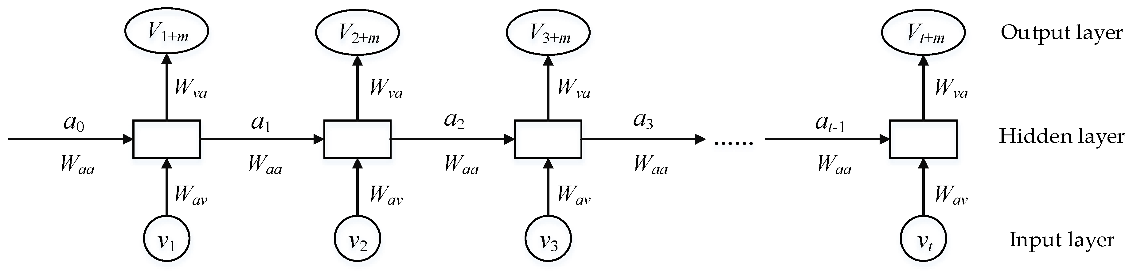
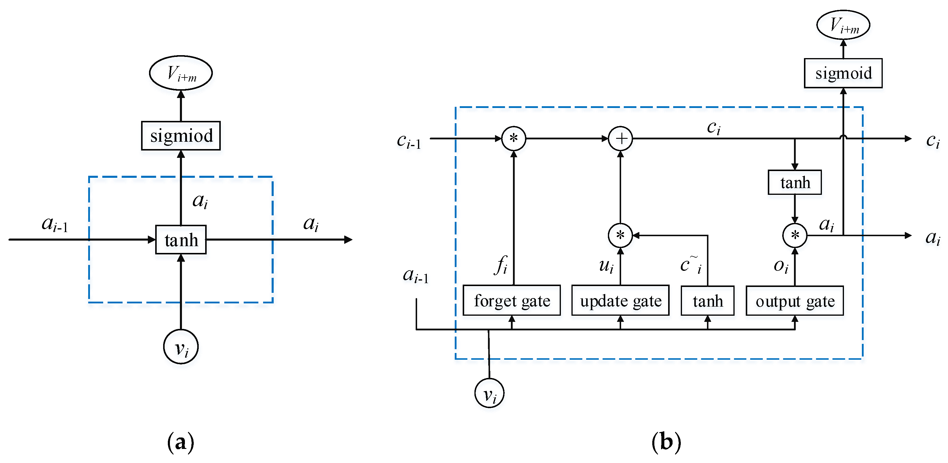
2.3. RNN and LSTMNN
3. The EEMD-FuzzyEn-LSTMNN Model
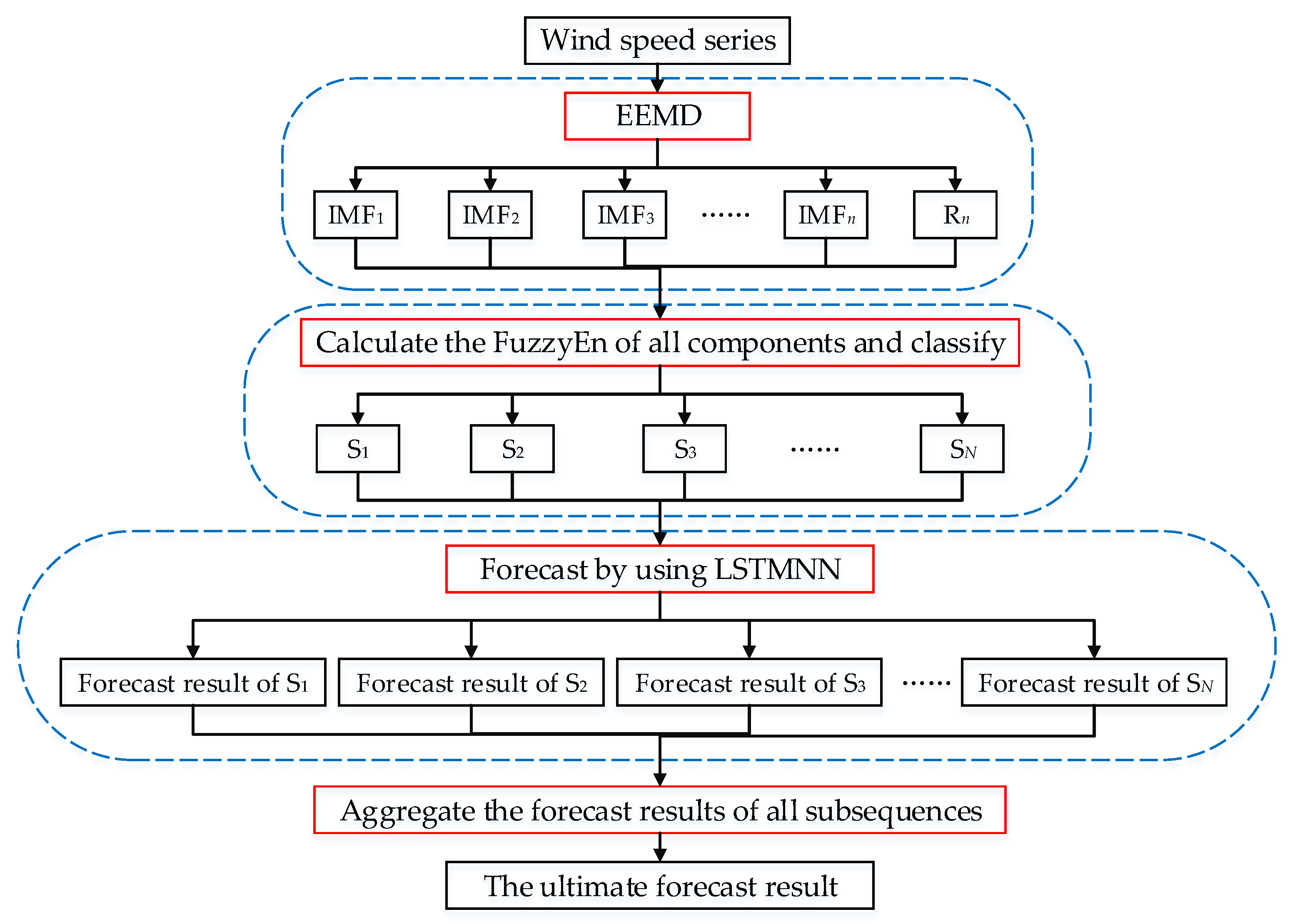
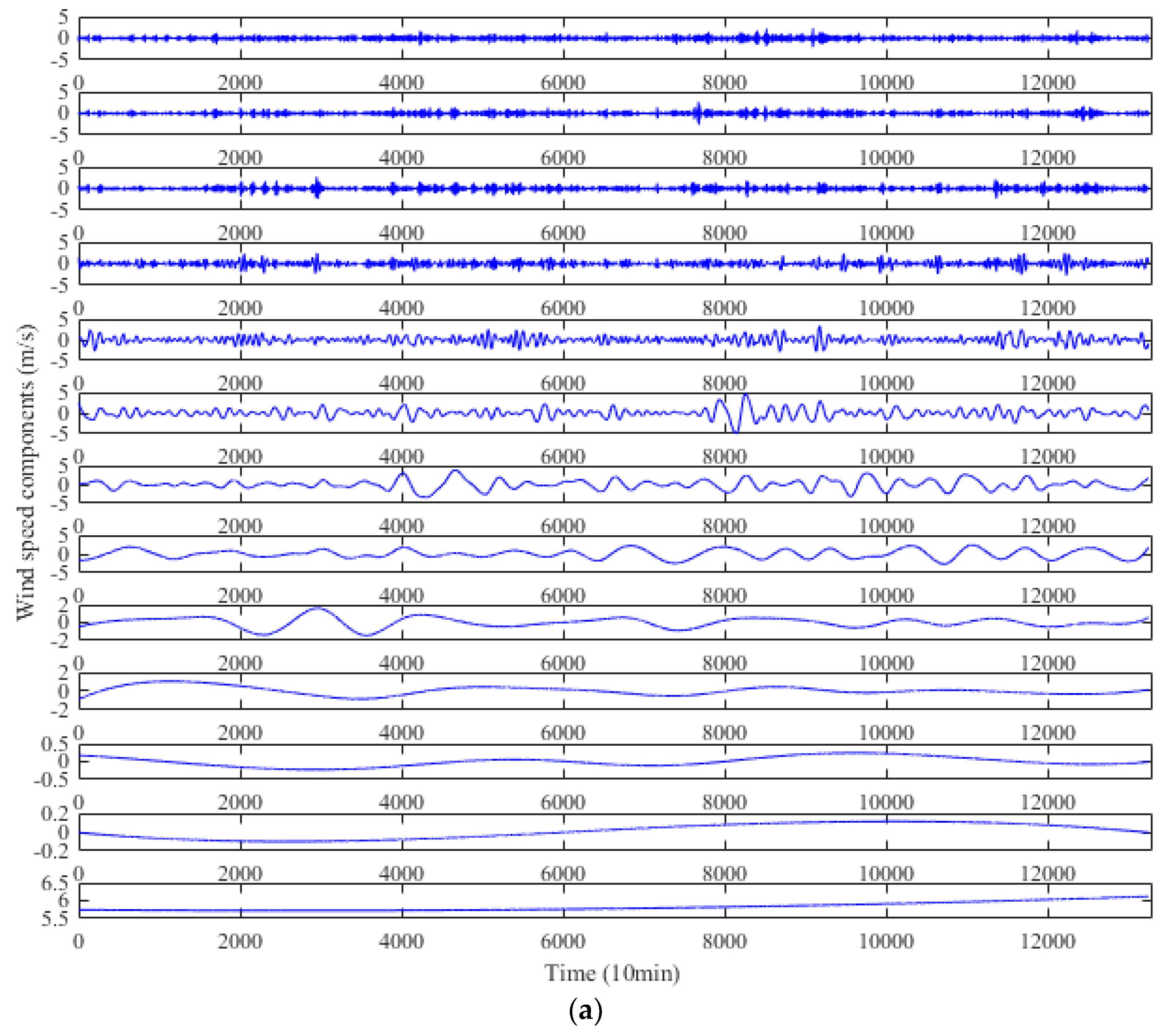
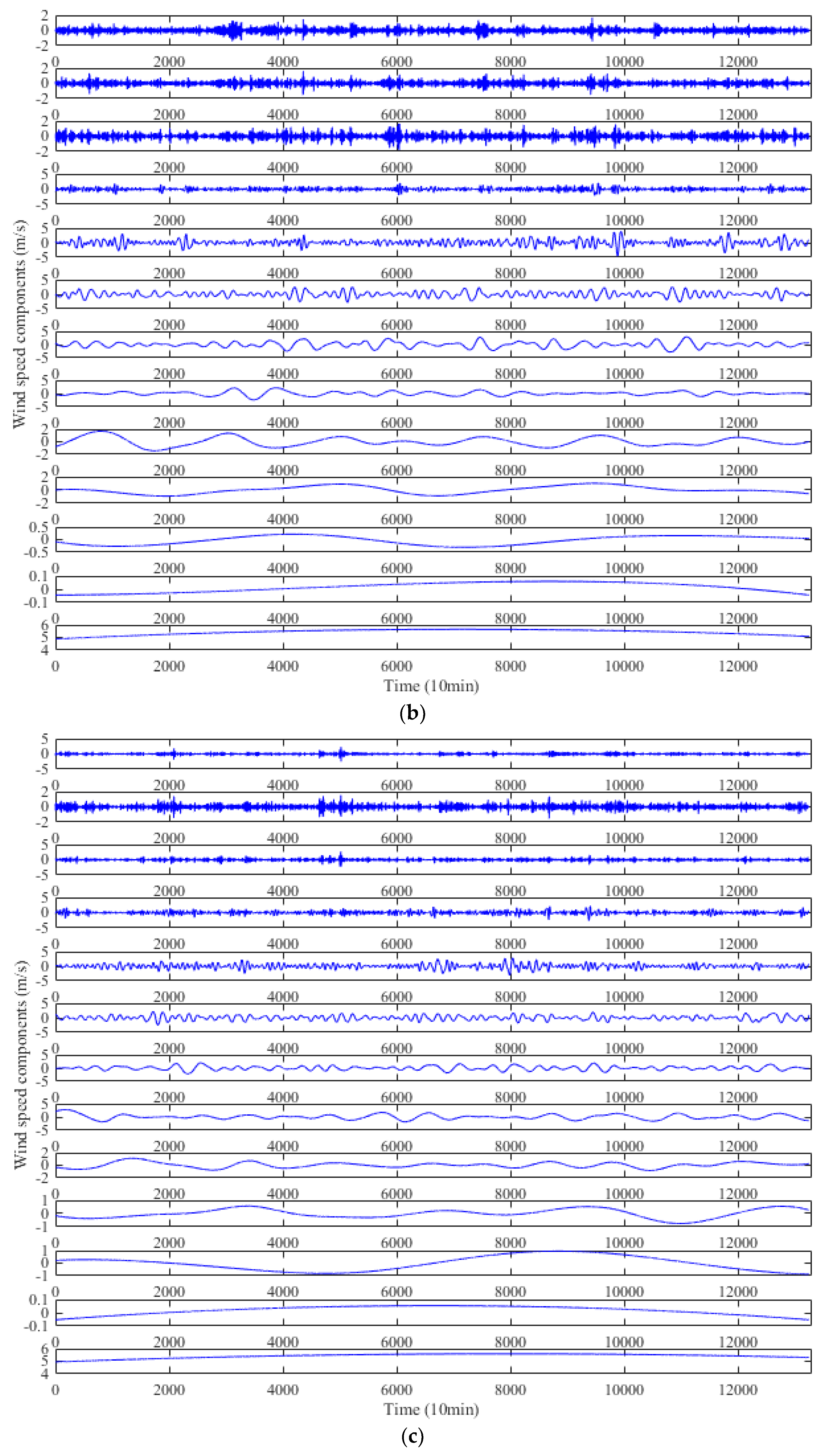
- Step 1: Use EEMD to decompose the original wind speed series into a number of IFM components and a residual component. These components are respectively denoted by IMF1, IMF2, …, IMFn and Rn.
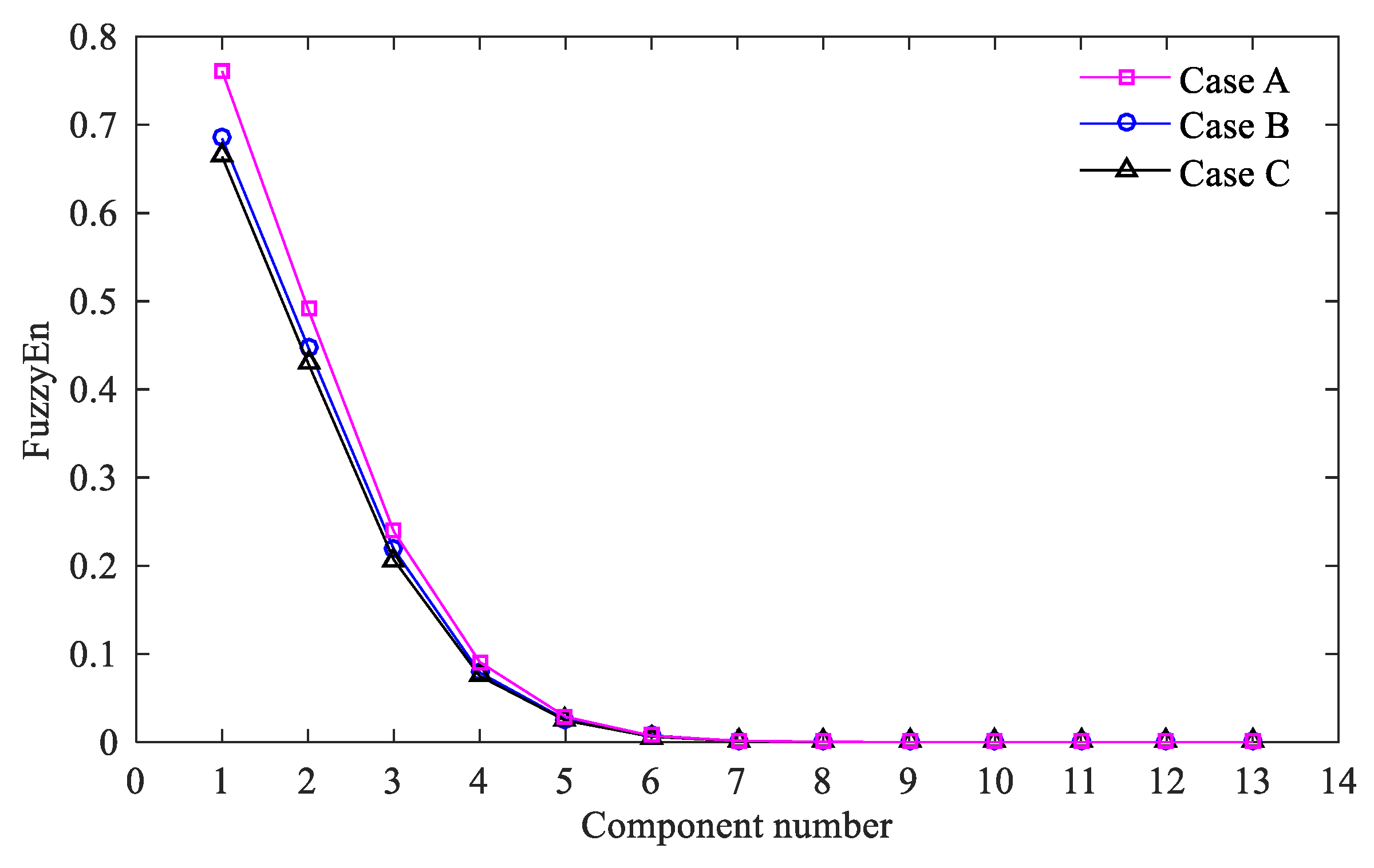
- Step 2: Calculate the FuzzyEn of each component and classify all components according to the calculated FuzzyEn values. The components with similar FuzzyEn values are classified into one group, and the components in one group are superimposed to obtain a new subsequence. All subsequences are respectively denoted by S1, S2, …, SN.
- Step 3: Use the LSTMNN model to forecast each subsequence separately.
- Step 4: Aggregate the forecasting result of each subsequence to obtain the ultimate forecasting series of wind speed.
4. The Predictable Time of Wind Speed Series
4.1. Selection of Wind Speed Series
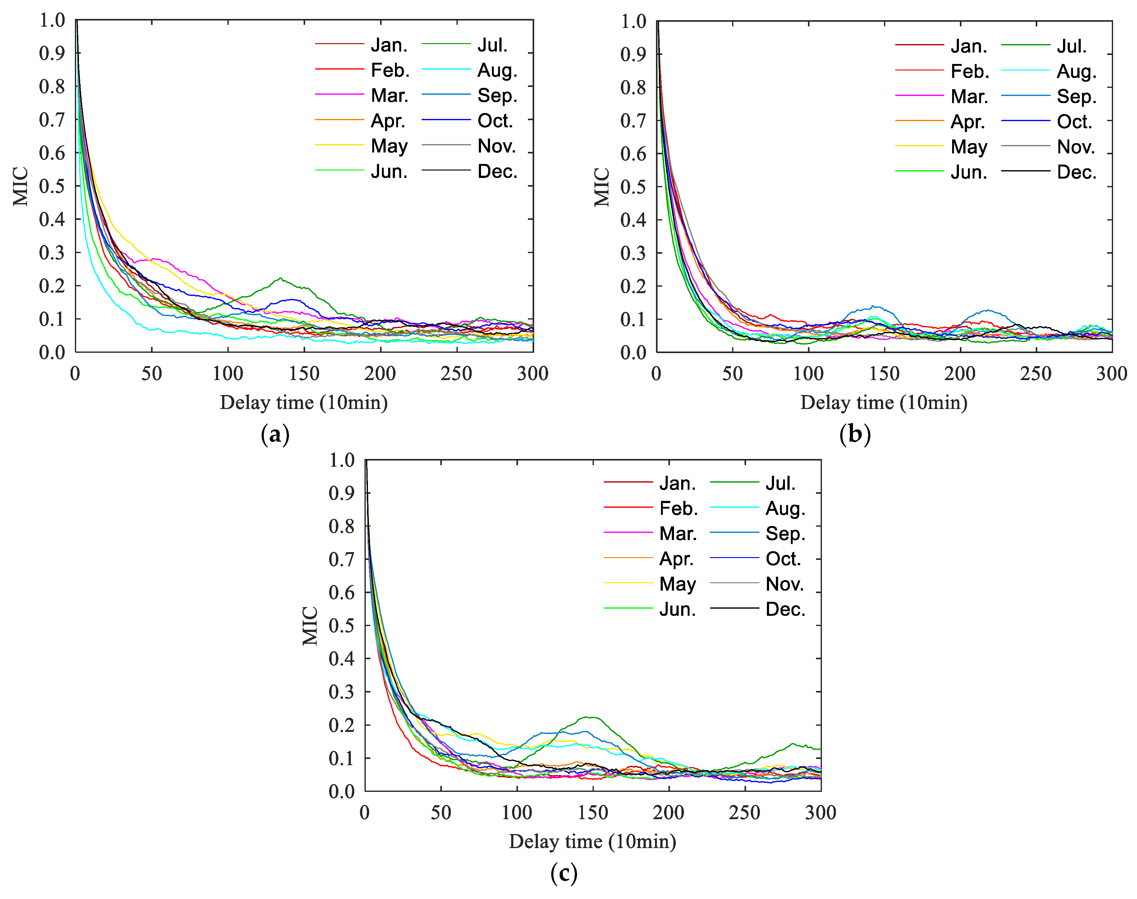
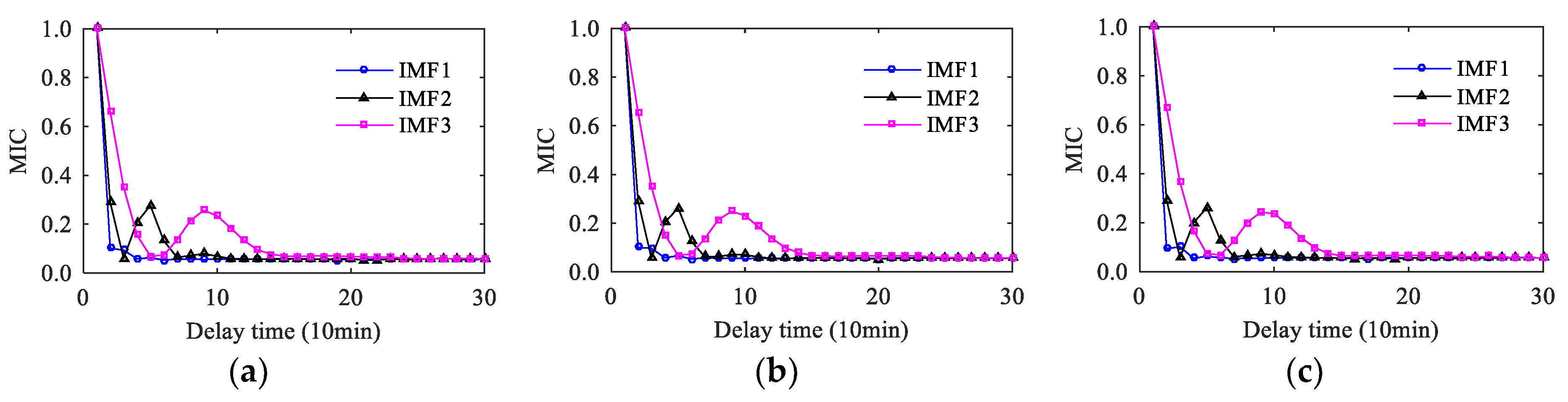
4.2. Autocorrelation Analysis of Wind Speed Series Based on MIC
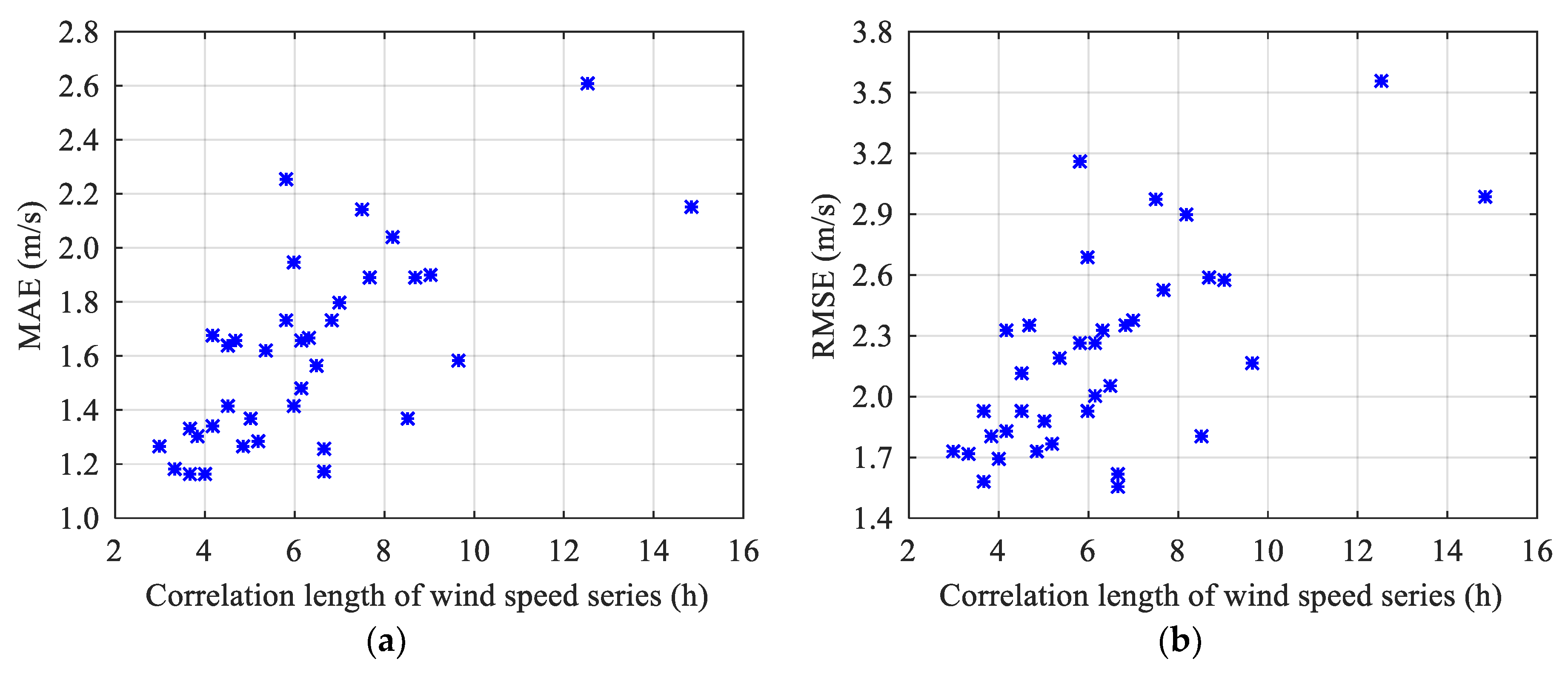
4.3. Analysis of Predictable Time
5. Case Study
5.1. Wind Speed Data Description of the Cases
5.2. Error Evaluation Index
5.3. Parameter Settings of the BPNN Model, the SVM Model and the LSTMNN Model
5.4. Decomposition Results by EEMD
5.5. Classification of Components Based on FuzzyEn
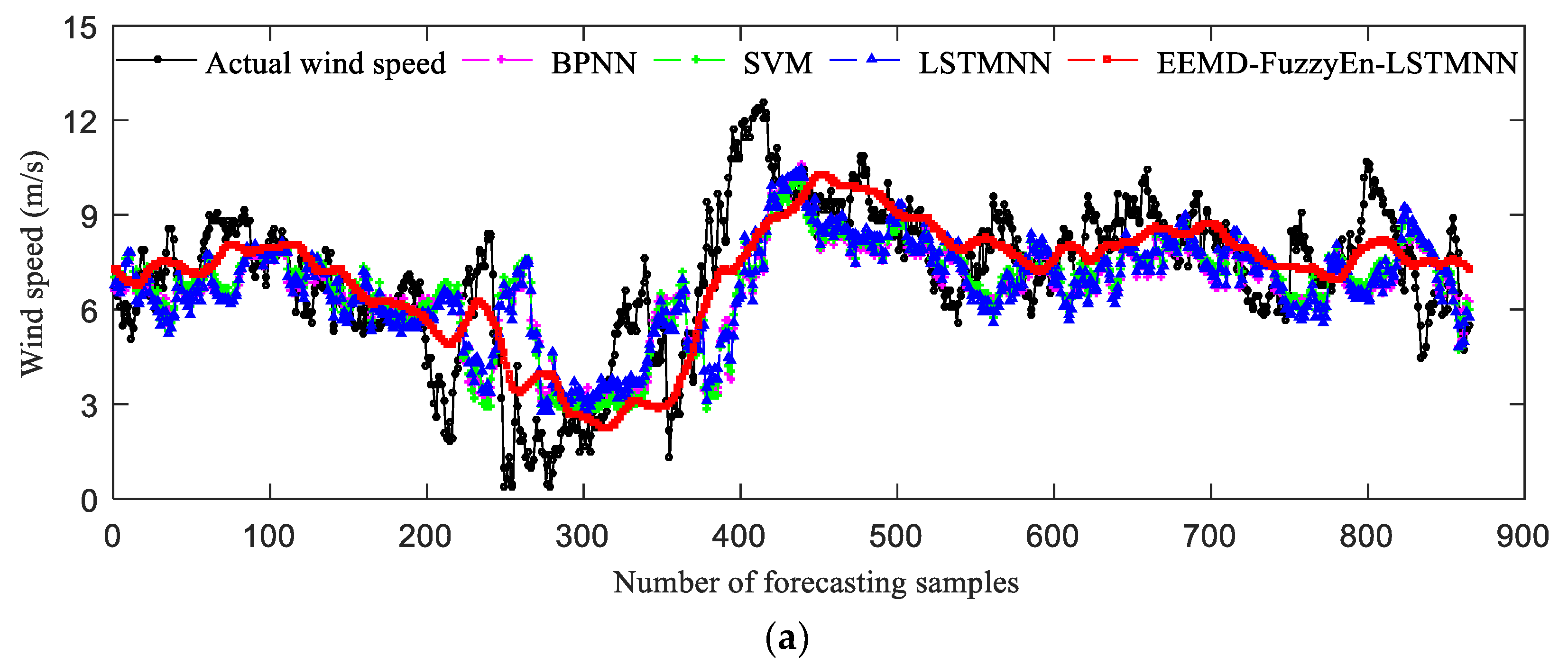
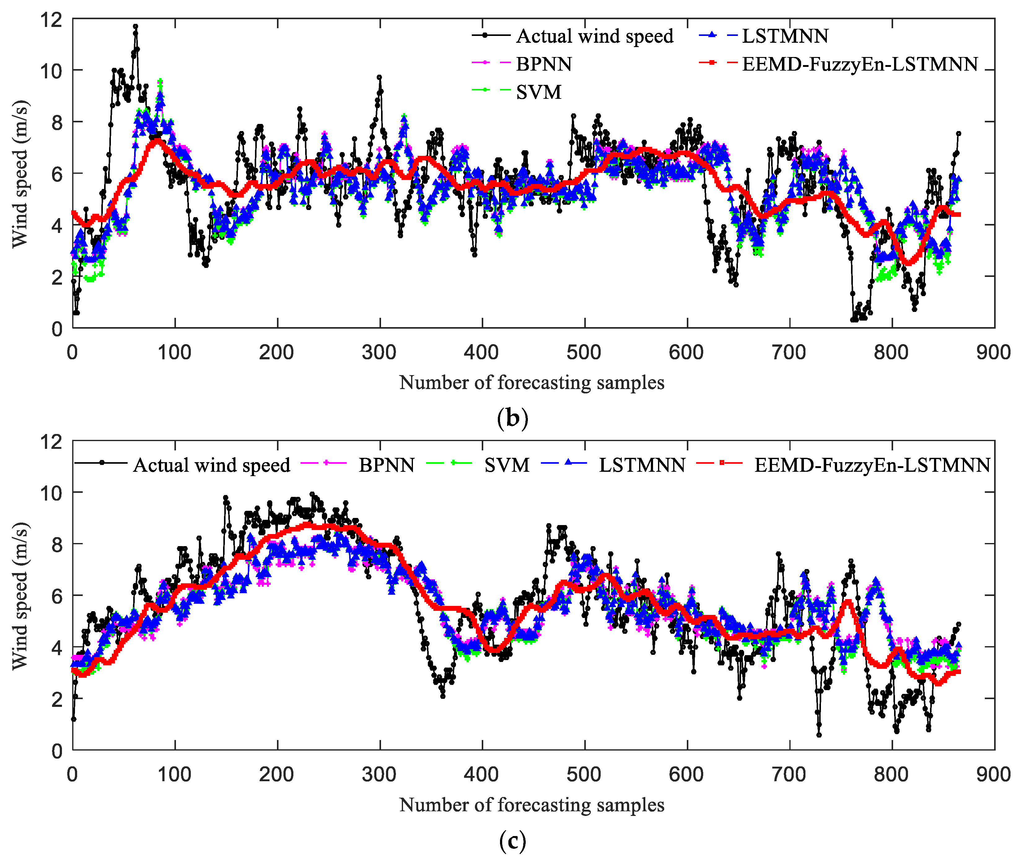
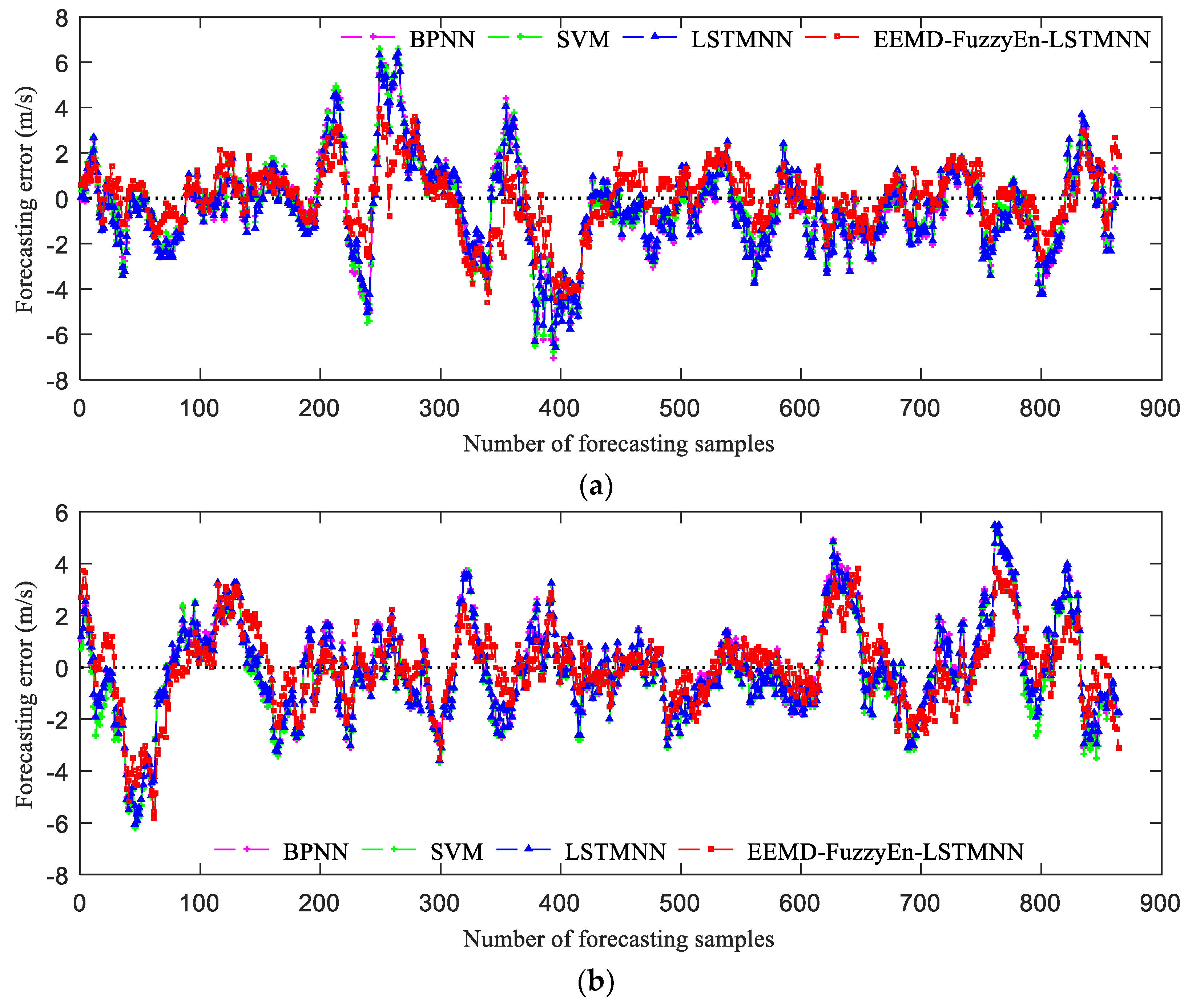
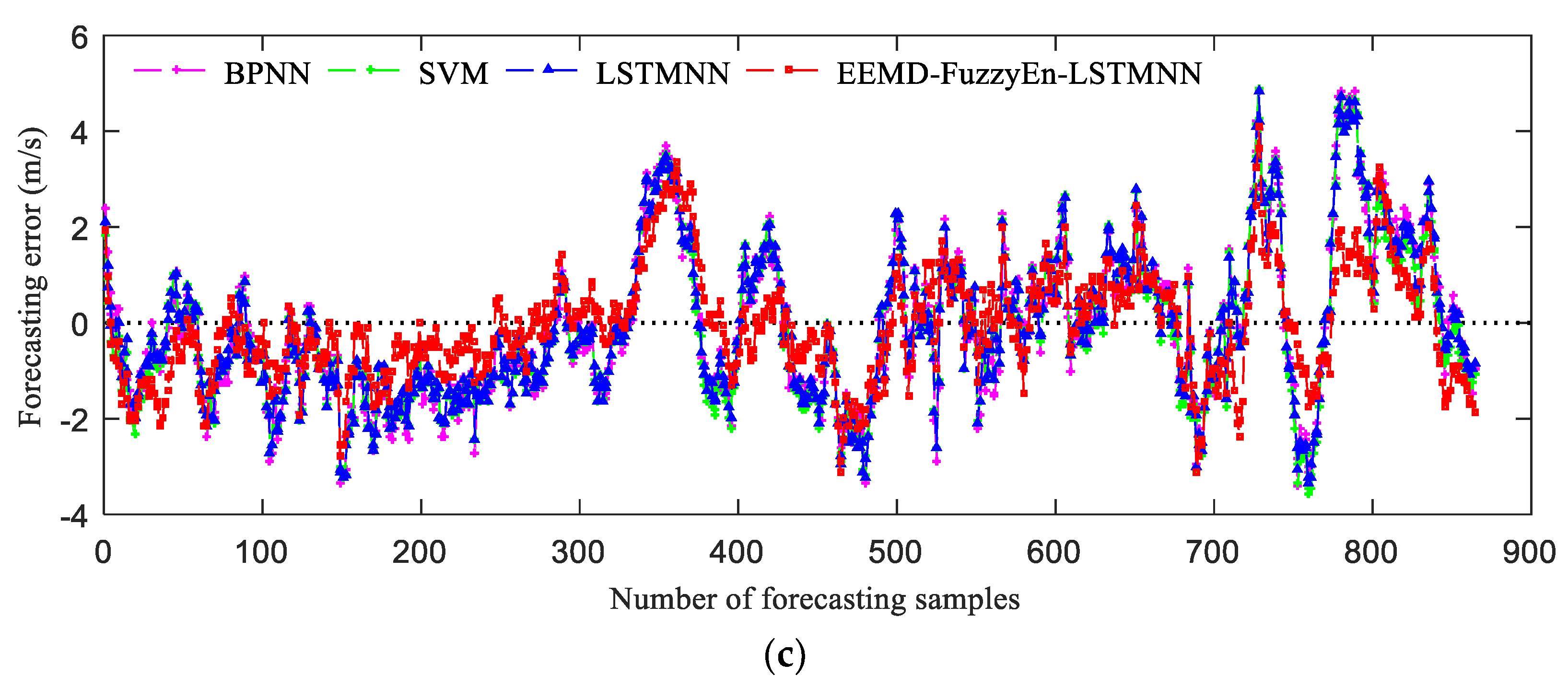
5.6. Forecasting Results and Analysis
6. Conclusions
- MIC is used to analyze the autocorrelation of wind speed series from different terrain conditions, and some suitable correlation lengths are obtained. As the correlation length of the wind speed series increases, the forecasting error tends to increase overall. The forecasting error analysis shows that four hours can be taken as the predictable time of the wind speed series for direct multistep forecasting based on historical wind speed data.
- The wind speed series from different terrain conditions is forecasted for the future four hours, and the forecasting accuracy of the LSTMNN model is slightly higher than that of the BPNN model and the SVM model. It shows that the LSTM neural network can make better use of the historical input information of the wind speed series, and it is more suitable for the wind speed statistical forecasting method.
- Under different terrain conditions, the forecasting accuracy of the EEMD-FuzzyEn-LSTMNN model is much higher than that of the LSTMNN model. Comparing the EEMD-FuzzyEn-LSTMNN model with the LSTMNN model, the MAE, MAPE and RMSE of the three cases are reduced by 0.2773–0.4413 m/s (19.74–29.18%), 0.0882–0.11 (21.74–29.7%), 0.3076–0.6014 m/s (16.81–30.04%), respectively. Moreover, the EEMD-FuzzyEn-LSTMNN model has more advantages for forecasting the wind speed series which has large forecasting errors by using ordinary neural networks.
Author Contributions
Funding
Conflicts of Interest
References
- Liu, H.; Tian, H.Q.; Chen, C.; Li, Y.F. An experimental investigation of two Wavelet-MLP hybrid frameworks for wind speed prediction using GA and PSO optimization. Electr. Power Energy Syst. 2013, 52, 161–173. [Google Scholar] [CrossRef]
- Jiang, P.; Wang, Y.; Wang, J.Z. Short-term wind speed forecasting using a hybrid model. Energy 2017, 119, 561–577. [Google Scholar] [CrossRef]
- Hu, J.M.; Wang, J.Z.; Zeng, G.W. A hybrid forecasting approach applied to wind speed time series. Renew. Energy 2013, 60, 185–194. [Google Scholar] [CrossRef]
- Chang, G.W.; Lu, H.J.; Chang, Y.R.; Lee, Y.D. An improved neural network-based approach for short-term wind speed and power forecast. Renew. Energy 2017, 105, 301–311. [Google Scholar] [CrossRef]
- Landberg, L. Short-term prediction of local wind conditions. J. Wind Eng. Ind. Aerodyn. 2001, 89, 235–245. [Google Scholar] [CrossRef]
- Martí, I.; Cabezón, D.; Villanueva, J.; Sanisidro, M.J.; Loureiro, Y.; Cantero, E.; Sanz, J. LocalPred and RegioPred. Advanced tools for wind energy prediction in complex terrain. In Proceedings of the 2003 European Wind Energy Conference and Exhibition, (EWEC’03), Madrid, Spain, 16–19 June 2003. [Google Scholar]
- Focken, U.; Lange, M.; Waldl, H.P. Previento-A wind power prediction system with an innovative upscaling algorithm. In Proceedings of the 2001 European Wind Energy Conference and Exhibition, (EWEC’01), Copenhagen, Denmark, 2–6 July 2001. [Google Scholar]
- Brown, B.G.; Katz, R.W.; Murphy, A.H. Time series models to simulate and forecast wind speed and wind power. J. Clim. Appl. Meteorol. 1984, 23, 1184–1195. [Google Scholar] [CrossRef]
- Torres, J.L.; García, A.; De Blas, M.; De Francisco, A. Forecast of hourly average wind speed with ARMA models in Navarre (Spain). Sol. Energy 2005, 79, 65–77. [Google Scholar] [CrossRef]
- El-Fouly, T.H.M.; El-Saadany, E.F.; Salama, M.M.A. Grey predictor for wind energy conversion systems output power prediction. IEEE Trans. Power Syst. 2006, 21, 1450–1452. [Google Scholar] [CrossRef]
- Mohandes, M.A.; Halawani, T.O.; Rehman, S.; Hussain, A.A. Support vector machines for wind speed prediction. Renew. Energy 2004, 29, 939–947. [Google Scholar] [CrossRef]
- Cadenas, E.; Rivera, W. Short term wind speed forecasting in La Venta, Oaxaca, México, using artificial neural networks. Renew. Energy 2009, 34, 274–278. [Google Scholar] [CrossRef]
- Flores, P.; Tapia, A.; Tapia, G. Application of a control algorithm for wind speed prediction and active power generation. Renew. Energy 2005, 30, 523–536. [Google Scholar] [CrossRef]
- Li, G.; Shi, J. On comparing three artificial neural networks for wind speed forecasting. Appl. Energy 2010, 87, 2313–2320. [Google Scholar] [CrossRef]
- Salcedo-Sanz, S.; Pérez-Bellido, Á.M.; Ortiz-García, E.G.; Portilla-Figueras, A.; Prieto, L.; Paredes, D. Hybridizing the fifth generation mesoscale model with artificial neural networks for short-term wind speed prediction. Renew. Energy 2009, 34, 1451–1457. [Google Scholar] [CrossRef]
- Ortiz-García, E.G.; Salcedo-Sanz, S.; Pérez-Bellido, Á.M.; Gascón-Moreno, J.; Portilla-Figueras, J.A.; Prieto, L. Short-term wind speed prediction in wind farms based on banks of support vector machines. Wind Energy 2011, 14, 193–207. [Google Scholar] [CrossRef]
- Giorgi, M.G.D.; Ficarella, A.; Tarantino, M. Assessment of the benefits of numerical weather predictions in wind power forecasting based on statistical methods. Energy 2011, 36, 3968–3978. [Google Scholar] [CrossRef]
- Wang, D.Y.; Luo, H.Y.; Grunder, O.; Lin, Y.B. Multi-step ahead wind speed forecasting using an improved wavelet neural network combining variational mode decomposition and phase space reconstruction. Renew. Energy 2017, 113, 1345–1358. [Google Scholar] [CrossRef]
- Yang, H.F.; Jiang, Z.P.; Lu, H.Y. A hybrid wind speed forecasting system based on a ‘decomposition and ensemble’ strategy and fuzzy time series. Energies 2017, 10, 1422. [Google Scholar] [CrossRef]
- Liu, H.; Tian, H.Q.; Pan, D.F.; Li, Y.F. Forecasting models for wind speed using wavelet, wavelet packet, time series and Artificial Neural Networks. Appl. Energy 2013, 107, 191–208. [Google Scholar] [CrossRef]
- Guo, Z.H.; Zhao, W.G.; Lu, H.Y.; Wang, J.Z. Multi-step forecasting for wind speed using a modified EMD-based artificial neural network model. Renew. Energy 2012, 37, 241–249. [Google Scholar] [CrossRef]
- Liu, H.; Chen, C.; Tian, H.Q.; Li, Y.F. A hybrid model for wind speed prediction using empirical mode decomposition and artificial neural networks. Renew. Energy 2012, 48, 545–556. [Google Scholar] [CrossRef]
- Huang, N.E.; Shen, Z.; Long, S.R. A new view of nonlinear water waves: The Hilbert spectrum. Annu. Rev. Fluid Mech. 1999, 31, 417–457. [Google Scholar] [CrossRef]
- Wang, S.X.; Zhang, N.; Wu, L.; Wang, Y.M. Wind speed forecasting based on the hybrid ensemble empirical mode decomposition and GA-BP neural network method. Renew. Energy 2016, 94, 629–636. [Google Scholar] [CrossRef]
- Zhao, Z.; Chen, W.H.; Wu, X.M.; Chen, P.C.Y.; Liu, J.M. LSTM network: A deep learning approach for short-term traffic forecast. IET Intell. Transp. Syst. 2017, 11, 68–75. [Google Scholar] [CrossRef]
- Srivastava, S.; Lessmann, S. A comparative study of LSTM neural networks in forecasting day-ahead global horizontal irradiance with satellite data. Sol. Energy 2018, 162, 232–247. [Google Scholar] [CrossRef]
- Kim, H.Y.; Won, C.H. Forecasting the volatility of stock price index: A hybrid model integrating LSTM with multiple GARCH-type models. Expert Syst. Appl. 2018, 103, 25–37. [Google Scholar] [CrossRef]
- Zhang, J.F.; Zhu, Y.; Zhang, X.P.; Ye, M.; Yang, J.Z. Developing a Long Short-Term Memory (LSTM) based model for predicting water table depth in agricultural areas. J. Hydrol. 2018, 561, 918–929. [Google Scholar] [CrossRef]
- Yu, J.; Kim, S. Locally-weighted polynomial neural network for daily short-term peak load forecasting. Int. J. Fuzzy Log. Intell. Syst. 2016, 16, 163–172. [Google Scholar] [CrossRef]
- Huang, N.E.; Shen, Z.; Long, S.R.; Wu, M.C.; Shih, H.H.; Zheng, Q.; Yen, N.C.; Tung, C.C.; Liu, H.H. The empirical mode decomposition and the Hilbert spectrum for nonlinear and non-stationary time series analysis. Proc. Math. Phys. Eng. Sci. 1998, 454, 903–995. [Google Scholar] [CrossRef]
- Wang, J.J.; Zhang, W.Y.; Li, Y.N.; Wang, J.Z.; Dang, Z.L. Forecasting wind speed using empirical mode decomposition and Elman neural network. Appl. Soft Comput. 2014, 23, 452–459. [Google Scholar] [CrossRef]
- Wu, Z.H.; Huang, N.E. A study of the characteristics of white noise using the empirical mode decomposition method. Proc. Math. Phys. Eng. Sci. 2004, 460, 1597–1611. [Google Scholar] [CrossRef]
- Wu, Z.H.; Huang, N.E. Ensemble Empirical Mode Decomposition: A noise-assisted data analysis method. Adv. Adapt. Data Anal. 2009, 1, 1–41. [Google Scholar] [CrossRef]
- Chen, W.T.; Wang, Z.Z.; Xie, H.B.; Yu, W.X. Characterization of surface EMG signal based on fuzzy entropy. IEEE Trans. Neural Syst. Rehabil. Eng. 2007, 15, 266–272. [Google Scholar] [CrossRef] [PubMed]
- Grzegorzewski, P. On separability of fuzzy relations. Int. J. Fuzzy Log. Intell. Syst. 2017, 17, 137–144. [Google Scholar] [CrossRef]
- Novák, V. Detection of structural breaks in time series using fuzzy techniques. Int. J. Fuzzy Log. Intell. Syst. 2018, 18, 1–12. [Google Scholar] [CrossRef]
- Bengio, Y.; Simard, P.Y.; Frasconi, P. Learning long-term dependencies with gradient descent is difficult. IEEE Trans. Neural Netw. 1994, 5, 157–166. [Google Scholar] [CrossRef] [PubMed]
- Hochreiter, S.; Schmidhuber, J. Long Short-term Memory. Neural Comput. 1997, 9, 1735–1780. [Google Scholar] [CrossRef] [PubMed]
- Gers, F.A.; Schmidhuber, J.; Cummins, F. Learning to forget: Continual prediction with LSTM. In Proceedings of the 9th International Conference on Artificial Neural Networks, (ICANN’99), Edinburgh, UK, 7–10 September 1999. [Google Scholar]
- Werbos, P.J. Backpropagation through time: What it does and how to do it. Proc. IEEE 1990, 78, 1550–1560. [Google Scholar] [CrossRef]
- Reshef, D.N.; Reshef, Y.A.; Finucane, H.K.; Grossman, S.R.; Mcvean, G.; Turnbaugh, P.J.; Lander, E.S.; Mitzenmacher, M.; Sabeti, P.C. Detecting novel associations in large data sets. Science 2011, 334, 1518–1524. [Google Scholar] [CrossRef]
- Madsen, H.; Pinson, P.; Kariniotakis, G.; Nielsen, H.A.; Nielsen, T.S. Standardizing the performance evaluation of short-term wind power prediction models. Wind Eng. 2005, 29, 475–489. [Google Scholar] [CrossRef]


| Number | Location | Local Terrain Condition | Selected Time of Wind Speed Series | Height of Wind Speed Measurement (m) |
|---|---|---|---|---|
| 1 | Hunan province | Mountainous area | From April 2014 to March 2015 | 80 |
| 2 | Henan province | Plain area | From June 2016 to May 2017 | 120 |
| 3 | Zhejiang province | Coastal area | From August 2011 to July 2012 | 100 |
| Month | Correlation Length (h) | ||
|---|---|---|---|
| Anemometer Tower 1 | Anemometer Tower 2 | Anemometer Tower 3 | |
| January | 8.17 | 6.17 | 6.67 |
| February | 5.83 | 5.83 | 3.67 |
| March | 14.83 | 4.50 | 6.83 |
| April | 7.50 | 6.00 | 4.67 |
| May | 12.50 | 4.17 | 6.17 |
| June | 4.50 | 3.67 | 4.83 |
| July | 7.00 | 3.33 | 5.33 |
| August | 3.00 | 4.00 | 8.67 |
| September | 6.33 | 3.83 | 6.67 |
| October | 9.67 | 6.00 | 5.17 |
| November | 7.67 | 6.50 | 5.00 |
| December | 9.00 | 4.17 | 8.50 |
| Forecasting Models | Parameters | Number or Type |
|---|---|---|
| BPNN model | Number of neurons in the hidden layer | 20 |
| Learning rate of training | 0.001 | |
| Training target | 0.00001 | |
| SVM model | Type of svm | epsilon-SVR |
| Type of kernel function | linear kernel function | |
| LSTMNN model | Number of neurons in the LSTM layer | 20 |
| Type of activation function of the output layer | tanh | |
| Optimizer | adam | |
| Learning rate | 0.0001 |
| Case | Forecasting models | MAE (m/s) | MAPE | RMSE (m/s) |
|---|---|---|---|---|
| Case A | BPNN model | 1.5308 | 0.3800 | 2.0371 |
| SVM model | 1.5264 | 0.3742 | 2.0211 | |
| LSTMNN model | 1.5122 | 0.3704 | 2.0022 | |
| EEMD-FuzzyEn-LSTMNN model | 1.0709 | 0.2604 | 1.4008 | |
| Case B | BPNN model | 1.4406 | 0.4875 | 1.8626 |
| SVM model | 1.4523 | 0.4861 | 1.8694 | |
| LSTMNN model | 1.4045 | 0.4835 | 1.8295 | |
| EEMD-FuzzyEn-LSTMNN model | 1.1272 | 0.3784 | 1.5219 | |
| Case C | BPNN model | 1.2697 | 0.3397 | 1.5798 |
| SVM model | 1.2733 | 0.3374 | 1.5767 | |
| LSTMNN model | 1.2585 | 0.3358 | 1.5624 | |
| EEMD-FuzzyEn-LSTMNN model | 0.9188 | 0.2476 | 1.1615 |
© 2019 by the authors. Licensee MDPI, Basel, Switzerland. This article is an open access article distributed under the terms and conditions of the Creative Commons Attribution (CC BY) license (http://creativecommons.org/licenses/by/4.0/).
Share and Cite
Qin, Q.; Lai, X.; Zou, J. Direct Multistep Wind Speed Forecasting Using LSTM Neural Network Combining EEMD and Fuzzy Entropy. Appl. Sci. 2019, 9, 126. https://doi.org/10.3390/app9010126
Qin Q, Lai X, Zou J. Direct Multistep Wind Speed Forecasting Using LSTM Neural Network Combining EEMD and Fuzzy Entropy. Applied Sciences. 2019; 9(1):126. https://doi.org/10.3390/app9010126
Chicago/Turabian StyleQin, Qiong, Xu Lai, and Jin Zou. 2019. "Direct Multistep Wind Speed Forecasting Using LSTM Neural Network Combining EEMD and Fuzzy Entropy" Applied Sciences 9, no. 1: 126. https://doi.org/10.3390/app9010126