Regarding Solid Oxide Fuel Cells Simulation through Artificial Intelligence: A Neural Networks Application

 ,
,  ,
,
Abstract
:Featured Application
Abstract
1. Introduction
2. Materials and Methods
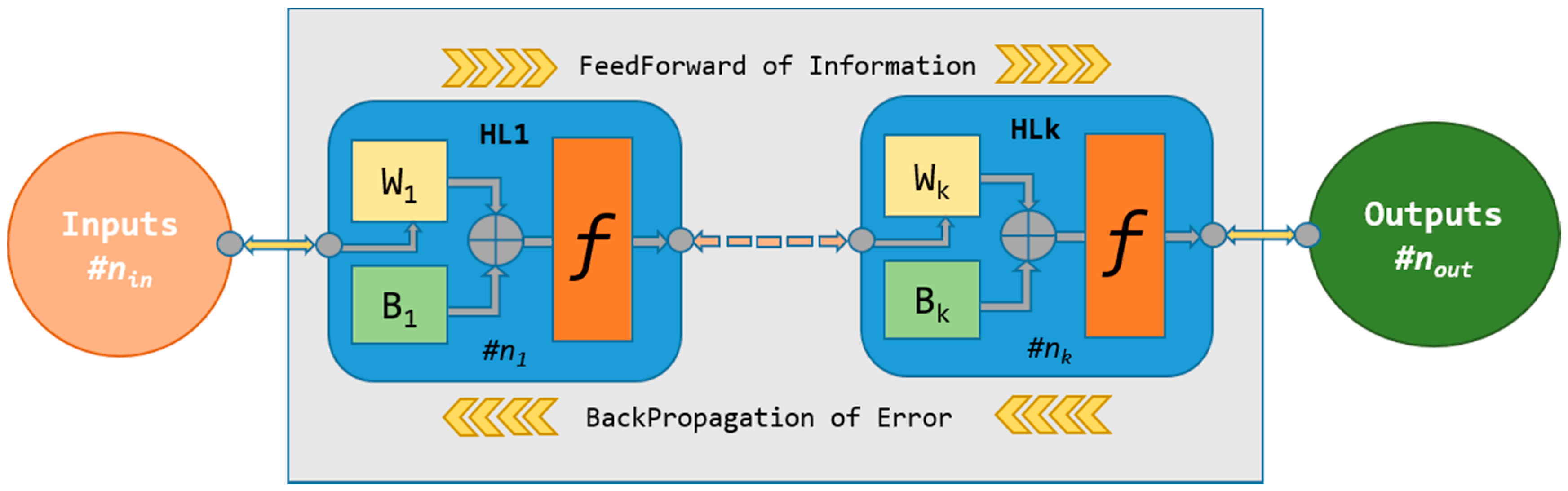
2.1. Artificial Neural Network Development
2.1.1. Architecture Definition
2.1.2. Training
- The first subset (70% of samples) is used for the training itself and it is fed to the network algorithm in order to calculate the values associated to the weight and bias matrix elements;
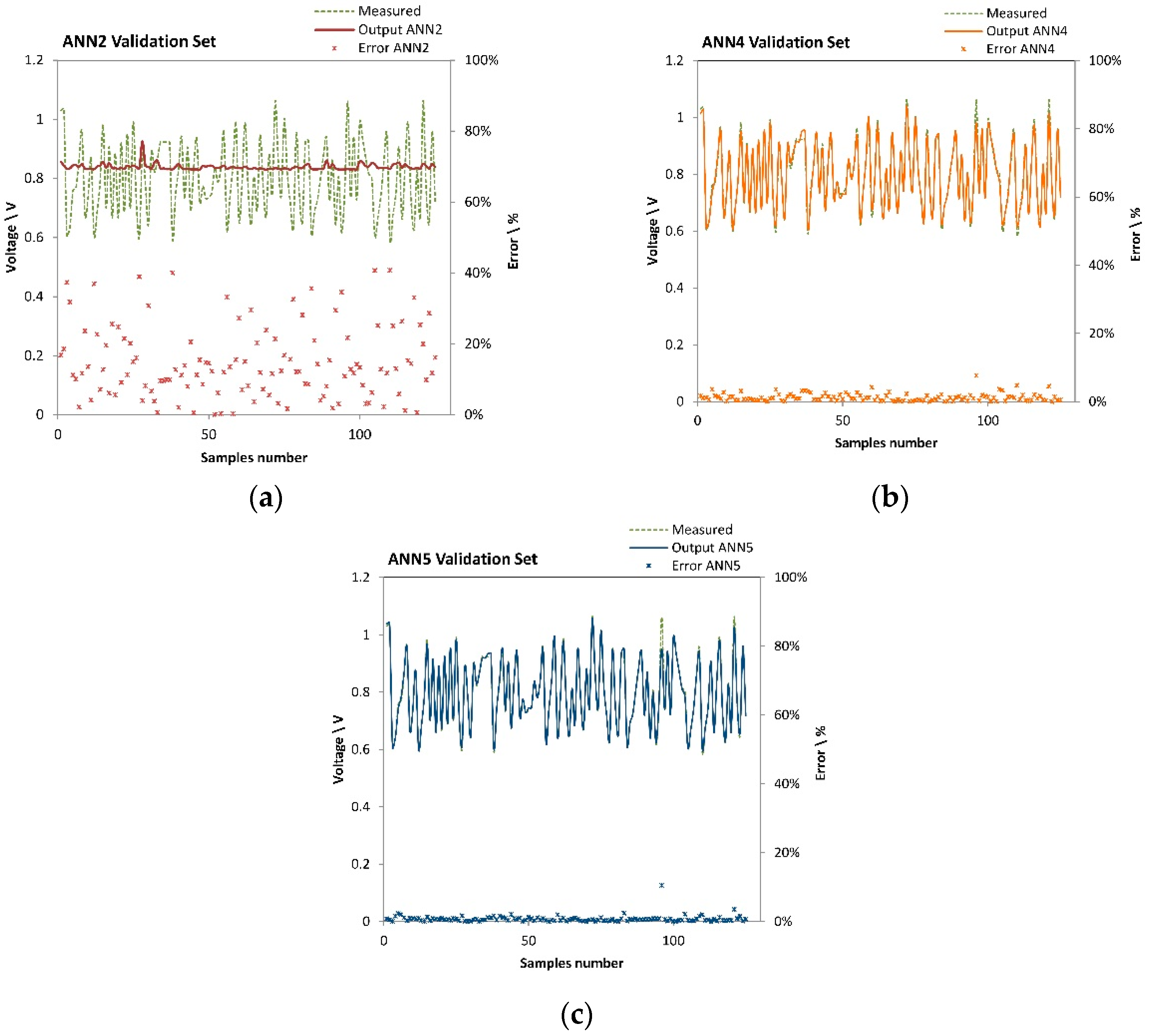
- The second subset (15% of samples) is used as validation basis. This is employed to measure the generalization capability of the network and to abort the training process early if the network performance on this subset does not improve. (i.e., before the target value for the error function is reached). The validation subset does not influence the network generalization capabilities.
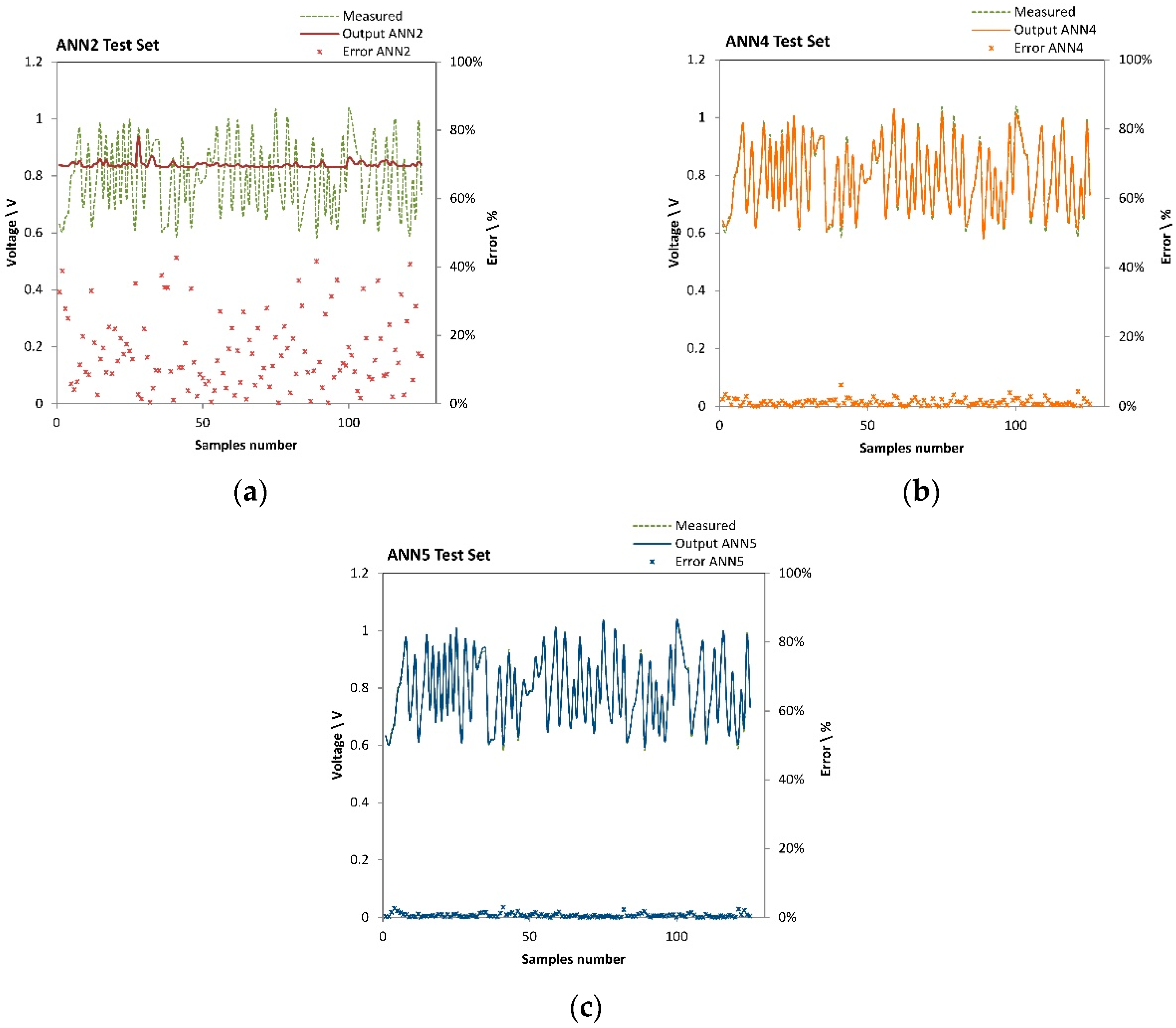
- The third subset (15% of samples) is used for the test, that is to say for a further generalization capability check having no effect on the training phase.
2.2. Experimental Data Collection
2.2.1. Materials and Experimental Set-Up
2.2.2. Design of Experiments
2.2.3. Tests Execution: Methods
3. Results
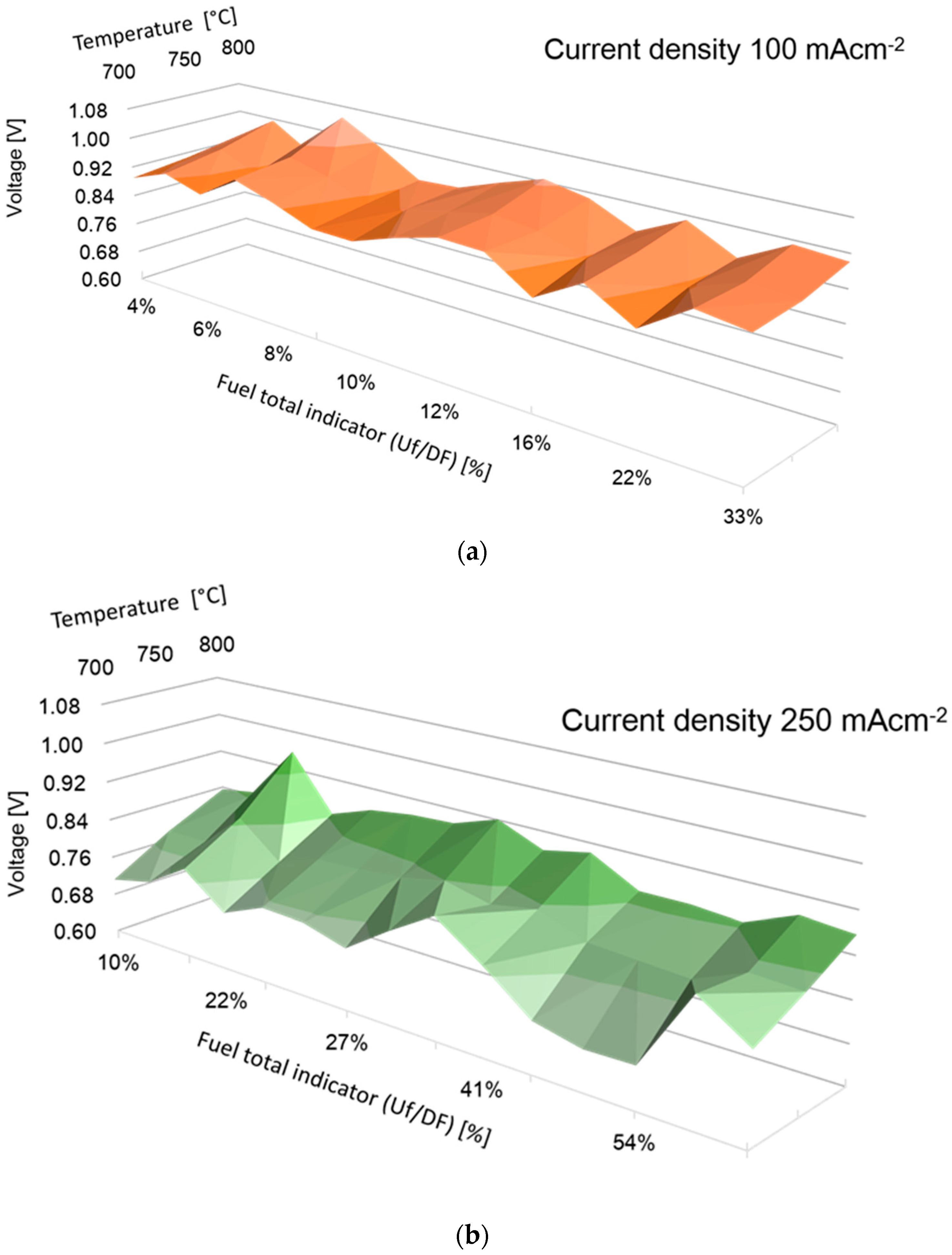
3.1. Experimental
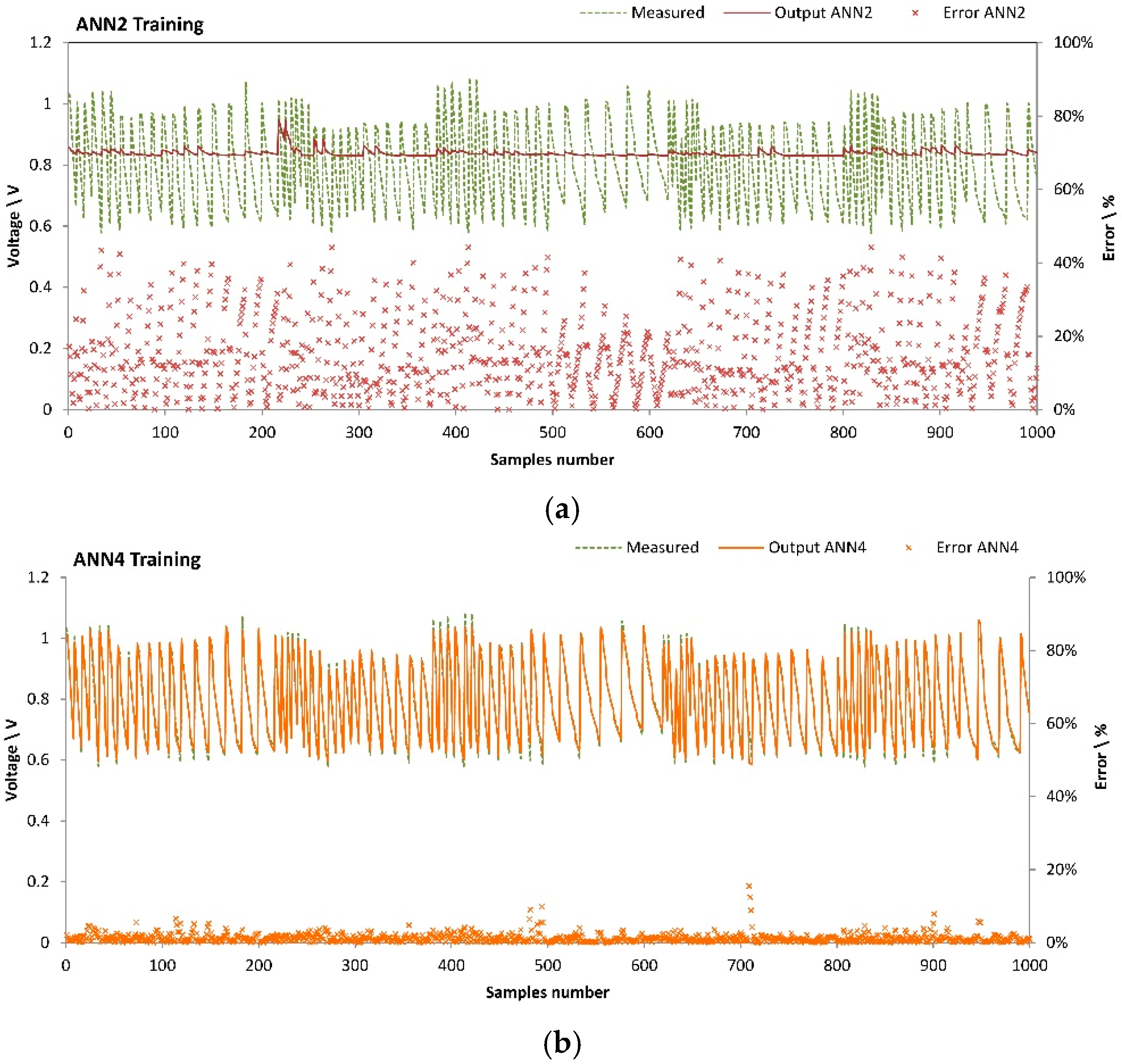
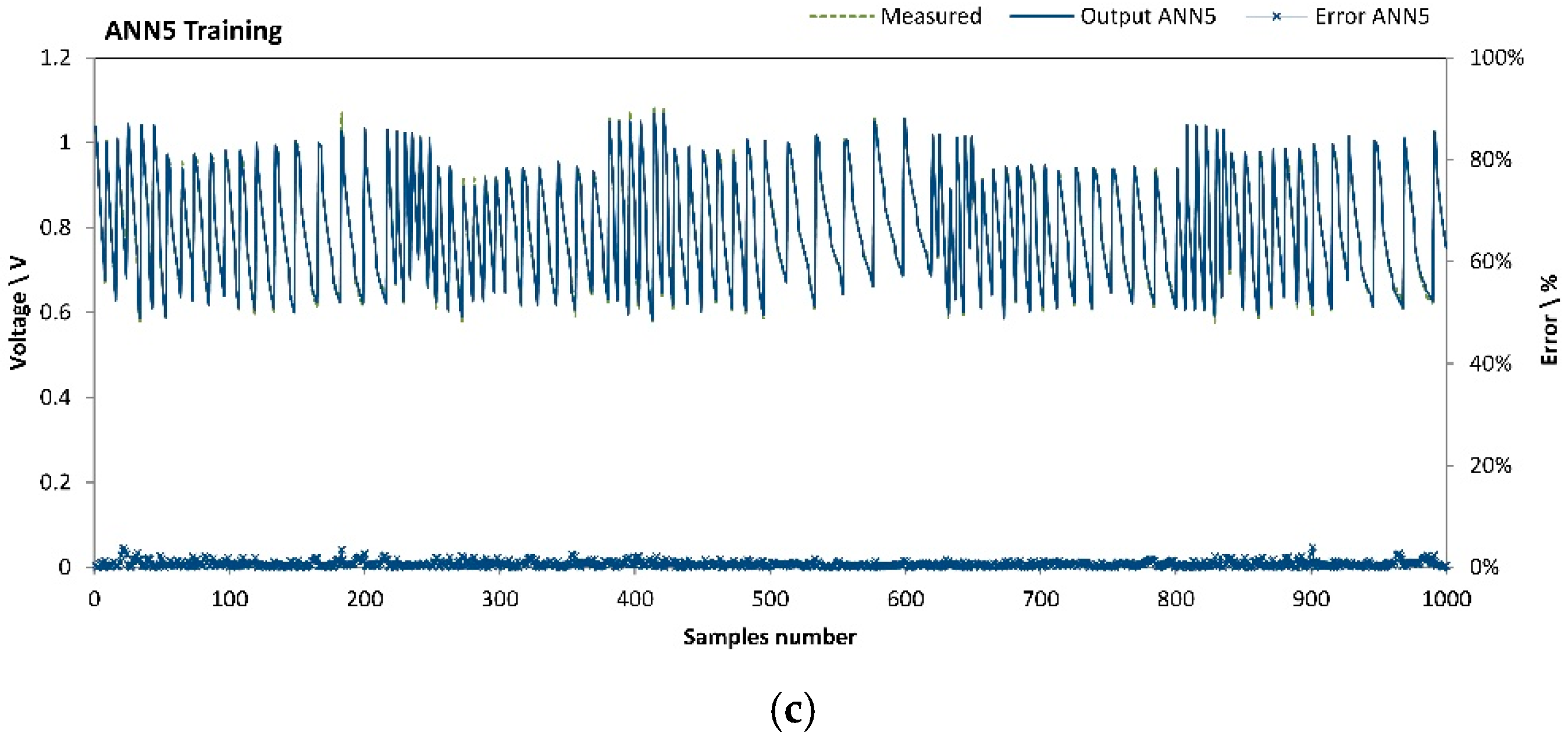
3.2. Neural Network Development
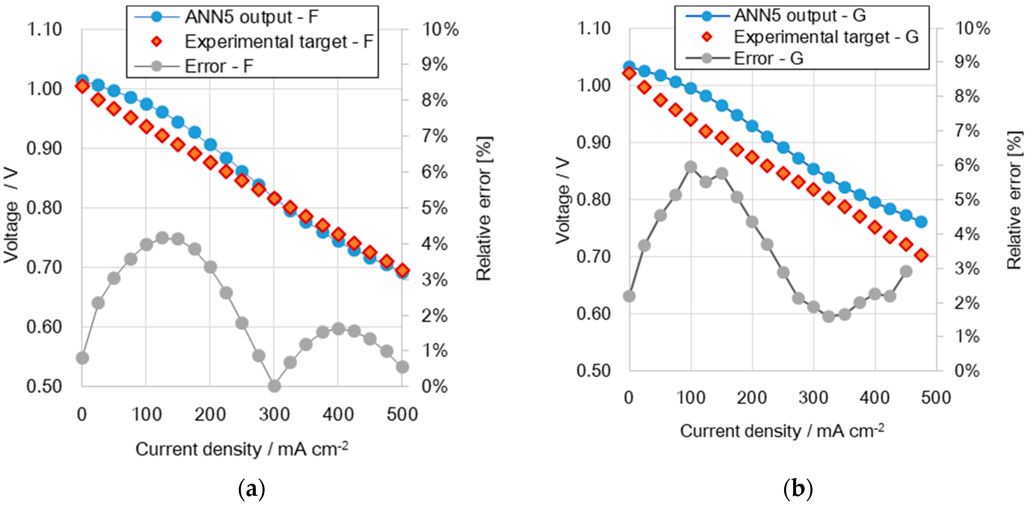
3.3. Neural Network Application
4. Conclusions
Author Contributions
Funding
Acknowledgments
Conflicts of Interest
References
- Suzuki, K. Industrial and Control Engineering Applications. In Artificial Neural Networks; InTechOpen, 2011; p. 490. Available online: https://www.intechopen.com/books/artificial-neural-networks-industrial-and-control-engineering-applications (accessed on 20 November 2017). [CrossRef]
- Deng, J.; Stobart, R.; Maass, B. The Applications of Artificial Neural Networks to Engines. In Artificial Neural Networks—Industrial and Control Engineering Applications; Loughborough University: Loughborough, UK, 2012; p. 450. [Google Scholar]
- Basheer, I.A.; Hajmeer, M. Artificial neural networks: Fundamentals, computing, design and application. J. Microbiol. Methods 2000, 43, 3–31. [Google Scholar] [CrossRef]
- Raza, M.Q.; Nadarajah, M.; Ekanayake, C. Demand forecast of PV integrated bioclimatic buildings using ensemble framework. Appl. Energy 2017, 208, 1626–1638. [Google Scholar] [CrossRef]
- Yildiz, B.; Bilbao, J.I.; Dore, J.; Sproul, A.B. Recent advances in the analysis of residential electricity consumption and applications of smart meter data. Appl. Energy 2017, 208, 402–427. [Google Scholar] [CrossRef]
- Ma, W.; Fang, S.; Liu, G.; Zhou, R. Modeling of district load forecasting for distributed energy system. Appl. Energy 2017, 204, 181–205. [Google Scholar] [CrossRef]
- Ahn, J.; Cho, S.; Chung, D.H. Analysis of energy and control efficiencies of fuzzy logic and artificial neural network technologies in the heating energy supply system responding to the changes of user demands. Appl. Energy 2017, 190, 222–231. [Google Scholar] [CrossRef]
- Sadough Vanini, Z.N.; Khorasani, K.; Meskin, N. Fault detection and isolation of a dual spool gas turbine engine using dynamic neural networks and multiple model approach. Inf. Sci. 2014, 259, 234–251. [Google Scholar] [CrossRef]
- Talaat, M.; Gobran, M.H.; Wasfi, M. A hybrid model of an artificial neural network with thermodynamic model for system diagnosis of electrical power plant gas turbine. Eng. Appl. Artif. Intell. 2018, 68, 222–235. [Google Scholar] [CrossRef]
- Tahan, M.; Tsoutsanis, E.; Muhammad, M.; Abdul Karim, Z.A. Performance-based health monitoring, diagnostics and prognostics for condition-based maintenance of gas turbines: A review. Appl. Energy 2017, 198, 122–144. [Google Scholar] [CrossRef] [Green Version]
- Davoudi, E.; Vaferi, B. Applying artificial neural networks for systematic estimation of degree of fouling in heat exchangers. Chem. Eng. Res. Des. 2018, 130, 138–153. [Google Scholar] [CrossRef]
- Barelli, L.; Bidini, G.; Bonucci, F. Diagnosis methodology for the turbocharger groups installed on a 1 MW internal combustion engine. Appl. Energy 2009, 86, 2721–2730. [Google Scholar] [CrossRef]
- Barelli, L.; Bidini, G.; Bonucci, F. Development of the regulation mapping of 1 MW internal combustion engine for diagnostic scopes. Appl. Energy 2009, 86, 1087–1104. [Google Scholar] [CrossRef]
- Barelli, L.; Bidini, G.; Bonucci, F. Diagnosis of a turbocharging system of 1 MW internal combustion engine. Energy Convers. Manag. 2013, 68, 28–39. [Google Scholar] [CrossRef]
- Barelli, L.; Bidini, G. Design of the measurements validation procedure and the expert system architecture for a cogeneration internal combustion engine. Appl. Therm. Eng. 2005, 25, 2698–2714. [Google Scholar] [CrossRef]
- European Commission. Communication from the Commission to the European Parliament, The Council, The European Economic and Social Committee, The Committee of the Regions and the European Investment Bank—Clean Energy for All Europeans; EU: Bruxelles, Belgium, 2017; Volume 14. [Google Scholar]
- IEA. Technology Roadmap: Energy Storage; International Energy Agency: Paris, France, 2014. [Google Scholar]
- Zhao, Y.; Liu, P.; Wang, Z.; Zhang, L.; Hong, J. Fault and defect diagnosis of battery for electric vehicles based on big data analysis methods. Appl. Energy 2017, 207, 354–362. [Google Scholar] [CrossRef]
- Xiang, C.; Ding, F.; Wang, W.; He, W. Energy management of a dual-mode power-split hybrid electric vehicle based on velocity prediction and nonlinear model predictive control. Appl. Energy 2017, 189, 640–653. [Google Scholar] [CrossRef]
- Daud, W.R.W.; Rosli, R.E.; Majlan, E.H.; Hamid, S.A.A.; Mohamed, R.; Husaini, T. PEM fuel cell system control: A review. Renew. Energy 2017, 113, 620–638. [Google Scholar] [CrossRef]
- Almeida, P.E.M.; Simões, M.G. Neural optimal control of PEM fuel cells with parametric CMAC networks. IEEE Trans. Ind. Appl. 2005, 41, 237–245. [Google Scholar] [CrossRef]
- Kheirandish, A.; Motlagh, F.; Shafiabady, N.; Dahari, M.; Khairi Abdul Wahab, A. Dynamic fuzzy cognitive network approach for modelling and control of PEM fuel cell for power electric bicycle system. Appl. Energy 2017, 202, 20–31. [Google Scholar] [CrossRef]
- Wu, G.; Sun, L.; Lee, K.Y. Disturbance rejection control of a fuel cell power plant in a grid-connected system. Control Eng. Pract. 2017, 60, 183–192. [Google Scholar] [CrossRef]
- Cheng, S.J.; Miao, J.M.; Wu, S.J. Use of metamodeling optimal approach promotes the performance of proton exchange membrane fuel cell (PEMFC). Appl. Energy 2013, 105, 161–169. [Google Scholar] [CrossRef]
- Madani, O.; Das, T. Feedforward based transient control in solid oxide fuel cells. Control Eng. Pract. 2016, 56, 86–91. [Google Scholar] [CrossRef] [Green Version]
- Tran, D.L.; Tran, Q.T.; Sakamoto, M.; Sasaki, K.; Shiratori, Y. Modelling of CH4 multiple-reforming within the Ni-YSZ anode of a solid oxide fuel cell. J. Power Sources 2017, 359, 507–519. [Google Scholar] [CrossRef]
- Chaichana, K.; Patcharavorachot, Y.; Chutichai, B.; Saebea, D.; Assabumrungrat, S.; Arpornwichanop, A. Neural network hybrid model of a direct internal reforming solid oxide fuel cell. Int. J. Hydrogen Energy 2012, 37, 2498–2508. [Google Scholar] [CrossRef]
- Milewski, J.; Świrski, K. Artificial Neural Network-Based Model for Calculating the Flow Composition Influence of Solid Oxide Fuel Cell. J. Fuel Cell Sci. Technol. 2013, 11, 021001. [Google Scholar] [CrossRef]
- Milewski, J.; Świrski, K. Modelling the SOFC behaviours by artificial neural network. Int. J. Hydrogen Energy 2009, 34, 5546–5553. [Google Scholar] [CrossRef]
- Wu, X.; Gao, D. Fault tolerance control of SOFC systems based on nonlinear model predictive control. Int. J. Hydrogen Energy 2017, 42, 2288–2308. [Google Scholar] [CrossRef]
- Jiang, Y.; Virkar, A.V. Fuel Composition and Diluent Effect on Gas Transport and Performance of Anode-Supported SOFCs. J. Electrochem. Soc. 2003, 150, A942–A951. [Google Scholar] [CrossRef]
- Virkar, A.V. Low Temperature Anode-Supported High Power Density Solid Oxide Fuel Cells with Nanostructured Electrodes; University of Utah: Salt Lake City, UT, USA, 2003. [Google Scholar] [CrossRef]
- Tjaden, B.; Gandiglio, M.; Lanzini, A.; Santarelli, M.; Ja, M. Small-Scale Biogas-SOFC Plant: Technical Analysis and Assessment of Di ff erent Fuel Reforming Options. Energy Fuels 2014, 28, 4216–4232. [Google Scholar] [CrossRef]
- Baldinelli, A.; Cinti, G.; Desideri, U.; Fantozzi, F. Biomass Integrated Gasifier-Fuel Cells: Experimental investigation on wood-syngas tars impact on SOFC anode materials. In Proceedings of the 11th EUROPEAN SOFC & SOE FORUM (EFCF Luzern), Lucerne, Switzerland, 1–4 July 2014. [Google Scholar]
- Rumelhart, D.E.; Hinton, G.E.; Williams, R.J. Learning internal representations by error propagation. In Parallel Data Process; Rumelhart, D.E., McClelland, J.L., Eds.; The MIT Press: Cambridge, MA, USA, 1986; pp. 318–362. [Google Scholar]
- Baldinelli, A.; Barelli, L.; Bidini, G.; Di Michele, A.; Vivani, R. SOFC direct fuelling with high-methane gases: Optimal strategies for fuel dilution and upgrade to avoid quick degradation. Energy Convers. Manag. 2016, 124, 492–503. [Google Scholar] [CrossRef]
- Baldinelli, A.; Cinti, G.; Desideri, U.; Fantozzi, F. Biomass integrated gasifier-fuel cells: Experimental investigation on wood syngas tars impact on NiYSZ-anode Solid Oxide Fuel Cells. Energy Convers. Manag. 2016, 128, 361–370. [Google Scholar] [CrossRef]
- Marie-Rose, S.C.; Perinet, A.L.; Lavoie, J. Conversion of Non-Homogeneous Biomass to Ultraclean Syngas and Catalytic Conversion to Ethanol. In Biofuel’s Engineering Process Technology; InTechOpen, 2008; Available online: https://www.intechopen.com/books/biofuel-s-engineering-process-technology/conversion-of-non-homogeneous-biomass-to-ultraclean-syngas-and-catalytic-conversion-to-ethanol/ (accessed on 12 November 2017).
- Baldinelli, A.; Barelli, L.; Bidini, G. Performance characterization and modelling of syngas-fed SOFCs (solid oxide fuel cells) varying fuel composition. Energy 2015, 90, 2070–2084. [Google Scholar] [CrossRef]
- Matsuka, M.; Shigedomi, K.; Ishihara, T. Comparative study of propane steam reforming in vanadium based catalytic membrane reactor with nickel-based catalysts. Int. J. Hydrogen Energy 2014, 39, 14792–14799. [Google Scholar] [CrossRef]
- The Biogas. Available online: http://www.biogas-renewable-energy.info/biogas_composition.html (accessed on 5 November 2017).
- Subotic, V.; Baldinelli, A.; Barelli, L.; Scharler, R. Optimization of an integrated biomass gasifier-fuel cell system: An experimental study on the cell response to process variations. In Proceedings of the Energy Procedia—10th International Conference on Applied Energy (ICAE2018), Hong Kong, China, 22–25 August 2018; pp. 22–25. [Google Scholar]


| ID | Architecture | Number of HL | Neurons in HL 1 | Neurons in HL 2 | Neurons in HL 3 | Neurons in HL 4 | Training Function | Transfer Function |
|---|---|---|---|---|---|---|---|---|
| ANN1 | L1 | 2 | 10 | 10 | - | - | TrainGDA | LogSIG |
| ANN2 | 2 | 16 | 12 | - | - | TrainGDM | ||
| ANN3 | 2 | 20 | 16 | - | - | |||
| ANN4 | L2 | 3 | 20 | 18 | 14 | - | TrainGDA | TanSIG |
| ANN5 | 3 | 25 | 22 | 18 | - | |||
| ANN6 | 3 | 15 | 10 | 10 | - | |||
| ANN7 | 3 | 25 | 20 | 22 | - | LogSIG | ||
| ANN8 | 3 | 30 | 28 | 26 | - | |||
| ANN9 | L3 | 4 | 12 | 10 | 8 | 6 | TanSIG | |
| ANN10 | L2 | 3 | 30 | 28 | 26 | - |
| Description | Symbol | Value |
|---|---|---|
| Minimum performance Gradient | - | 0.00001 |
| Maximum validation failures | - | 600 |
| Performance Goal | - | 0 |
| Learning rate | LR | 0.01 |
| Learning rate increasing ratio | LRinc | 1.05 |
| Learning rate decreasing ratio | LRdec | 0.7 |
| Temperature | Gas Mixture Volume Fraction on Dry Basis | j | |||||||
|---|---|---|---|---|---|---|---|---|---|
| °C | MIX | Ref. | H2 | CO | CH4 | CO2 | N2 | mL·min−1·cm−2 | mA·cm−2 |
| 700 750 800 | synA | [37] | 10% | 13% | 4% | 19% | 54% | 10.8 14.7 23.6 | 0 A → I (0.6 V) (Δj = 50 mA·cm−2) |
| synB | [38] | 48% | 0% | 14% | 9% | 29% | |||
| synC | [39] | 22% | 26% | 30% | 22% | 0% | |||
| synD | [40] | 32% | 38% | 0% | 30% | 0% | |||
| synE | [41] | 0% | 0% | 45% | 32% | 45% | |||
| ANN | Training | Validation | Test | Number of Learning Epochs | |
|---|---|---|---|---|---|
| ID | RMS % | MSE | RMS % | RMS % | |
| ANN1 | 10.75% | 0.0117 | 10.8% | 10.97% | 42 |
| ANN2 | 12.92% | 0.0169 | 13.0% | 12.86% | 31,000 |
| ANN3 | 13.02% | 0.0171 | 13.1% | 13.01% | 100,000 |
| ANN4 | 1.36% | 0.0002 | 1.4% | 1.21% | 10,600 |
| ANN5 | 0.80% | <0.0001 | 0.7% | 0.67% | 120,000 |
| ANN6 | 0.99% | <0.0001 | 1.0% | 1.05% | 100,000 |
| ANN7 | 1.01% | 0.0001 | 1.0% | 1.12% | 100,000 |
| ANN8 | 0.98% | <0.0001 | 1.0% | 1.07% | 100,000 |
| ANN9 | 1.10% | 0.0001 | 1.1% | 1.05% | 100,000 |
| ANN 10 | 0.75% | <0.0001 | 0.8% | 0.78% | 112,000 |
| Variables | Exp synF Settings | Exp synG Settings | ANN5 Input Range | ||||
|---|---|---|---|---|---|---|---|
| Min | Max | ||||||
| Temperature (°C) | 765 | 800 | 700 | 800 | |||
| Equivalent hydrogen flowrate (mL·min−1·cm−2) | 18.34 | 15.48 | 10.80 | 23.56 | |||
| Area Specific partial flowrates (mL·min−1·cm−2) | H2 | 3.67 | (20.0%vol) | 5.16 | (20.0%vol) | 0 | 10.51 |
| CO | 7.34 | (40.0%vol) | 5.16 | (20.0%vol) | 0 | 12.74 | |
| CO2 | 2.75 | (15.0%vol) | 3.87 | (15.0%vol) | 0 | 5.73 | |
| CH4 | 1.83 | (10.0%vol) | 1.29 | (5.0%vol) | 1.27 | 11.46 | |
| N2 | 2.75 | (15.0%vol) | 10.32 | (40.0%vol) | 0 | 32.17 | |
| Current density (mA·cm−2) | 0–500 | 0–500 | 0 | 1300 | |||
© 2018 by the authors. Licensee MDPI, Basel, Switzerland. This article is an open access article distributed under the terms and conditions of the Creative Commons Attribution (CC BY) license (http://creativecommons.org/licenses/by/4.0/).
Share and Cite
Baldinelli, A.; Barelli, L.; Bidini, G.; Bonucci, F.; Iskenderoğlu, F.C. Regarding Solid Oxide Fuel Cells Simulation through Artificial Intelligence: A Neural Networks Application. Appl. Sci. 2019, 9, 51. https://doi.org/10.3390/app9010051
Baldinelli A, Barelli L, Bidini G, Bonucci F, Iskenderoğlu FC. Regarding Solid Oxide Fuel Cells Simulation through Artificial Intelligence: A Neural Networks Application. Applied Sciences. 2019; 9(1):51. https://doi.org/10.3390/app9010051
Chicago/Turabian StyleBaldinelli, Arianna, Linda Barelli, Gianni Bidini, Fabio Bonucci, and Feride Cansu Iskenderoğlu. 2019. "Regarding Solid Oxide Fuel Cells Simulation through Artificial Intelligence: A Neural Networks Application" Applied Sciences 9, no. 1: 51. https://doi.org/10.3390/app9010051