A Feasibility Study of the Drive-By Method for Damage Detection in Railway Bridges


1
Dipartimento di Meccanica, Politecnico di Milano, Via La Masa 1, 20156 Milano, Italy
2
Department of Electromechanical Engineering Technology, KU Leuven, Gebroeders De Smetstraat 1, 9000 Ghent, Belgium
*
Author to whom correspondence should be addressed.
Appl. Sci. 2019, 9(1), 160; https://doi.org/10.3390/app9010160
Submission received: 1 November 2018
/
Revised: 11 December 2018
/
Accepted: 20 December 2018
/
Published: 4 January 2019
(This article belongs to the Special Issue Fault Detection and Diagnosis in Mechatronics Systems)
Abstract
:Damage identification and localization in railway bridges is a widely studied topic. Strain, displacement, or acceleration sensors installed on the bridge structure are normally used to detect changes in the global behavior of the structure, whereas approaches like ultra-sonic testing, acoustic emission, and magnetic inspection are used to check a small portion of structure near localized damage. The aim of this paper is to explore another perspective for monitoring the structural status of railway bridges, i.e., to detect structural damage from the dynamic response of the train transiting the bridge. This approach can successfully be implemented in the case of resonant bridges, thanks to the high level of acceleration generated, but its application becomes more challenging when the excitation frequencies due to train passage do not excite the first mode of vibration of the bridge. The paper investigates the feasibility of the method in the latter case, through numerical simulations of the complete train-track-bridge system. Accelerations on axleboxes and bogies are processed through suitable algorithms to detect differences arising when the train crosses a defective bridge or a healthy one. The results outline the main operational parameters affecting the method, the best placement for sensors, and the best frequency range to be considered in the signal processing, also addressing the issues that are related to track irregularity. Good performance can be achieved in the case of short bridges, but a few practical issues must be tackled before the method could be tested in practice.
1. Introduction
Health monitoring of railway bridges is gaining more and more interest in the management of railway assets, since most of the commuter networks date back many decades, and the requirement to increase speed and axle loads on existing lines poses new challenges to the maintenance of aged structures. Several kinds of instruments are proposed in the literature to measure bridge strains, accelerations, and displacements, and structural properties like natural frequencies, mode shapes, and modal parameters [1]. Some of the main ones to be mentioned are strain gauges and fiber optics, accelerometers, potentiometers, global positioning system (GPS) receivers, and vision systems for displacements. These measures are then adopted to assess the health state of the bridge, either through model-based or data-driven methods [1]. The monitoring of railway bridges through sensors installed on the structure is economically viable in the case of the main bridges or modern high-speed lines [2,3], but it is not practicable for the large number of bridges of different ages and types that are present in the main ordinary railway lines. These bridges are therefore usually monitored through periodic visual inspections, which nevertheless require a relevant effort in terms of manpower and time. Moreover, since visual inspections rely on human assessments, their outcomes can significantly vary, depending on the inspector. Between two following checks, no information regarding the health of the structure is gained, which can lead to a late detection of the damage, and to service disruption. In this respect, a continuous follow-up would be preferable.
The issue of how to assess the structural condition and integrity of many bridges of different ages and types in an affordable and efficient way is therefore a relevant topic, currently under discussion.
A recent perspective to monitor the structural status of railway bridges consists of so-called drive-by damage detection [4,5,6], i.e., the concept of directly using the transit of the train on the bridge as an excitation source, and sensors installed on the vehicle rather than on the bridge. A restricted number of commercial trains fitted with few sensors would enable the monitoring of the status of a great number of structures, using the train response to detect the presence of damage in the bridge. The detection method basically relies on the comparison of the acceleration data obtained from instrumented trains against a reference condition corresponding to the healthy structure; accelerations measured on train are processed through proper algorithms, which should be able to detect an alteration in the behavior of the train-track-bridge system.
If on the one hand, the drive-by method can successfully be implemented in the case of resonant bridges, thanks to the high level of acceleration generated when the train excites the natural frequency of the bridge [7], the application becomes more challenging when the first mode of vibration of the bridge is not relevantly excited by the train passage [5]. The main challenge in this case is the small difference in the acceleration levels to be detected, to discern a damaged structure from an undamaged structure, which may result in a low signal-to-noise ratio. Suspension stages from the bridge structure to the measuring vehicle, consisting of railway equipment, of the interface contact between wheel and rail, and finally of the train primary and secondary suspensions, represent an extra barrier that makes damage detection harder. For these reasons, a successful application of the drive-by method necessarily requires the investigation of the best position for sensor placement on-board train (i.e., axlebox, bogie frame, or carbody), and the implementation of a suitable algorithm for the analysis of the acceleration signals. This work presents the results of a plan of numerical simulations, intended to be an analysis of the different aspects which are likely to affect the applicability of the drive-by damage detection method. A numerical model for simulating the train–track–bridge interaction [8] is used, including the bridge structure, the track, and a multi-body model of the vehicle. Several conditions are simulated, considering different kinds of bridges, different train models, train speeds, damage levels, and locations of the damage along the bridge. The optimal sensor layout is investigated, to define the sensor position on the train that can deliver the most meaningful output to analyze the structural status of the bridge. Finally, the effect of track irregularity and ballast degradation on the reliability of the damage detection method is addressed.
Two different approaches can be investigated for data-processing, basically differing in the frequency range of the acceleration data considered. The first approach considered in this paper originates from the work described in González, A., & Hester, D. [9,10], focused on a bridge for road transportation. In the mentioned work, data generated by the vehicle passage are filtered to cancel the dynamic components due to the bridge modes of vibration, so that the remaining signal is representative of the quasi-static deflection of the bridge in response to the moving loads. The authors then define a damage component index that is suitable for damage identification, obtained by subtracting from the acceleration measured the reference response of the healthy structure.
A second approach may be intended to consider the entire dynamic response of the train–bridge system, in as wide a frequency range as possible. The presence of a defect alters indeed not only the quasi-static response, but also the dynamic response of the vehicle when the train passes by the structural defect, as well as the dynamic response of the bridge itself. In this paper, an analysis of the spectral components of train accelerations resulting from healthy and damage bridge is performed, and the results of a damage identification method based on moving window root mean square (RMS) are commented. Discussion on the applicability of the two methods, and limitations and influence of realistic operational parameters is carried out.
The paper is organized in the following points: in Section 2, the complete model for the train-track-bridge system is described; the bridge is modeled through the finite element method (FEM), while the full train is modeled as a multibody system. In Section 3, the simulation plan is described, and the two different data processing techniques are presented. Section 4 presents the simulation results in terms of the best positioning of sensors on the train, the acceleration levels to be measured, accuracy in the localization of the damage, and the effects of track irregularity on the feasibility of the method. Further necessary researches are mentioned, needed before the method could be tested in practice. Finally, in Section 5, conclusions are drawn, and the feasibility of the drive-by method is discussed.
2. Train–Track–Bridge Model
2.1. Railway Bridge Model
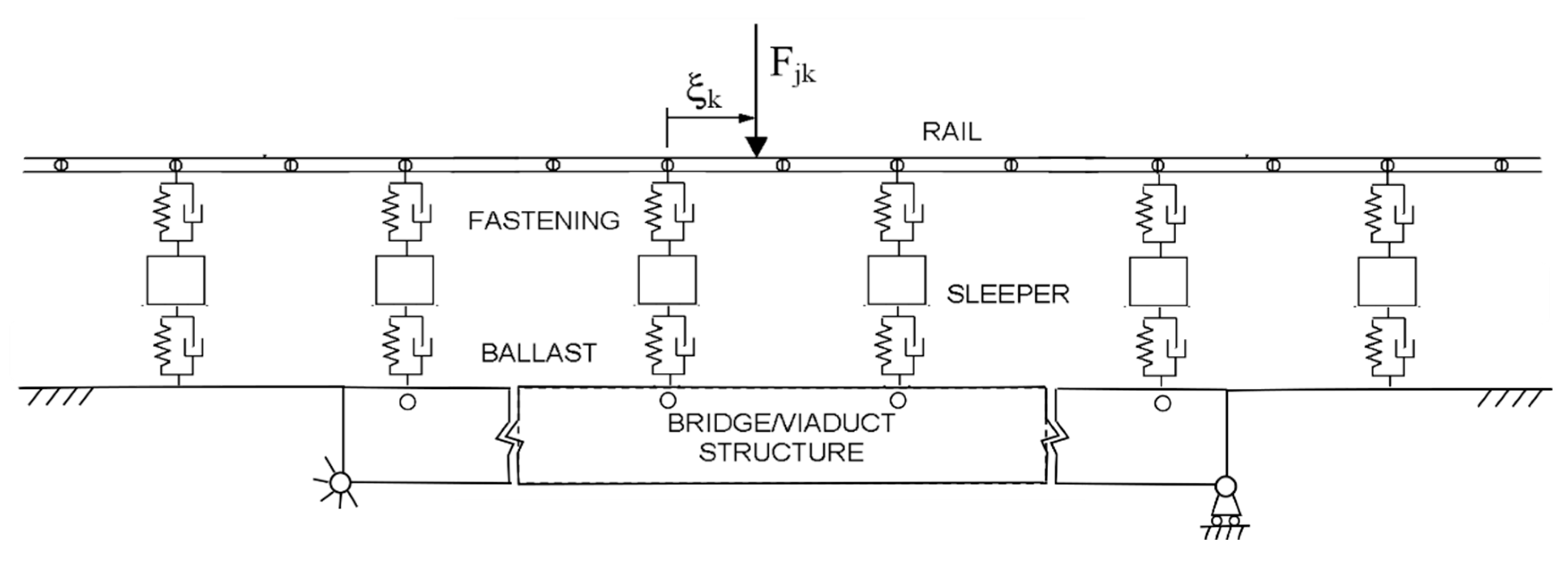
Each bridge is modeled as a simply supported beam, which is a typical configuration for railway bridges or multi-span viaducts. The bridge deck is modeled with Eulero–Bernoulli beams, and the complete model also includes the ballasted track above the bridge deck. Rails are modeled through finite elements, while sleepers are considered as rigid bodies and modeled with lumped masses (220 kg) and their moments of inertia, the frequency range of interest in the present analysis being up to 70 Hz. Two modules of ballasted track of length 29.4 m each are included before and after the bridge model (see Figure 1), to reproduce the continuity of the track, and to avoid introducing an artificial singularity between a fully rigid track and the bridge.
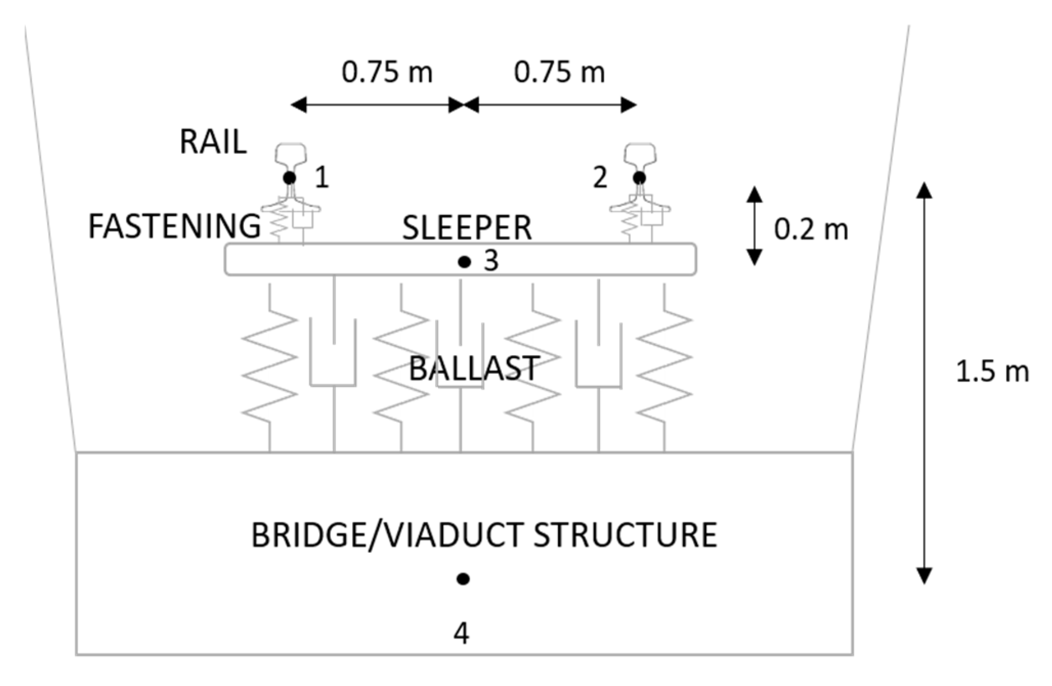
To form a track module, the beam nodes are spaced 0.6 m in the case of the rail, and 4.2 m for the bridge, so that seven rail elements correspond to each bridge beam element. Sleepers are spaced every 0.6 m, and therefore for every section containing rail nodes, there is a node representing a sleeper as a concentrated inertia.
The ballast is modeled by means of springs connecting the sleepers to the deck, also in the correspondence of sections in between the two nodes of each bridge beam element. The potential energy of the springs associated with these internal locations is calculated by means of the beam shape function. Figure 2 shows the scheme of the sections where both rails and bridge nodes are present. Nodes 1 and 2 are used to mesh the rails, node 4 to mesh bridge, and node 3 represents the sleeper.
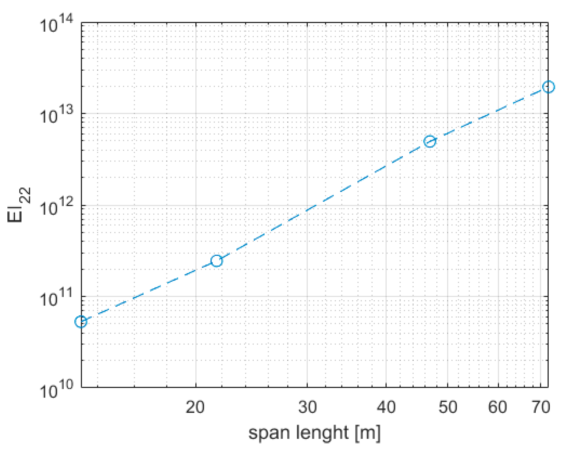
Four different structures are simulated, as to evaluate the performance of the drive-by method for different span lengths, flexural stiffnesses, and natural frequencies. Bridge models are named in the following, with numbers from #1 to #4, ordered with increasing span lengths. For all of the models, the Young’s modulus is equal to 206,000 MPa, and α and β Railegh coefficients to 0.1 and 0.2 × 10⁻³ respectively. In this paper, steel properties are considered, even if the proposed methodology can be extended to concrete bridges. Table 1 reports all the other bridge properties, together with the first flexural natural frequency f1 (I22 is the area moment of inertia along the horizontal axis and I33 is the area moment of inertia along the vertical axis). Bridges number one and two are short bridges: the first one is 13.2 m long, with a rather high fist natural frequency (i.e., 21.82 Hz), and the second one is 21.6 m long, with properties based on those of an existing bridge. The third bridge is a medium-long span bridge of length 46.8 m, and the last model has a long span (72 m), with properties derived from an existing bridge. Figure 3 reports the flexural stiffnesses EI22 of the four bridge models, as a function of span length. The dependence is a power coefficient that is equal to 3.5.
Table 2 reports the characteristics of the stiffnesses that are adopted for the connections between the sleepers and the bridge (k1 and k2, representing ballast), and for the connections between the rail nodes and the sleepers (k3 representing the stiffness properties of the fastenings). As for the ballast, stiffness k1 is adopted for bridge #2, whereas stiffness k2 is adopted for all the other bridges. As for the fastenings, the node-to-node spring k3 is used for all of the considered tracks.
To simulate the damage, each bridge is built with two modules with different mesh densities (apart from the shorter bridge #1). A coarse mesh of 4.2 m per element is adopted in sections that are not affected by the damage, whereas a module with a finer mesh of 1.2 m per element is adopted around the defective region. The structural damage is simulated through a reduction of the flexural stiffness in one of the 1.2 m-long beam elements [9,11], obtained by reducing the Young modulus of the material. To allow for a comparison between the structural response of the damaged bridge and that of the healthy bridge, the module with finer mesh is also included in the healthy bridge in the same location as in the damaged model.
The equation of motion of the bridge/rail structure [8] is formulated by means of the finite element method, obtaining the following equation:
where is the vector with the degrees of freedom (d.o.f) of the bridge/rail structure, [MS] represents the global mass matrix, [CS] the global damping matrix and [KS] the global stiffness matrix. is the vector of contact forces between the structure, in correspondence of the rail, and the vehicle in correspondence of the wheels [8,12], depending on the degrees of freedom of the rail () and of the i-th vehicle (from to ).
2.2. Train Model
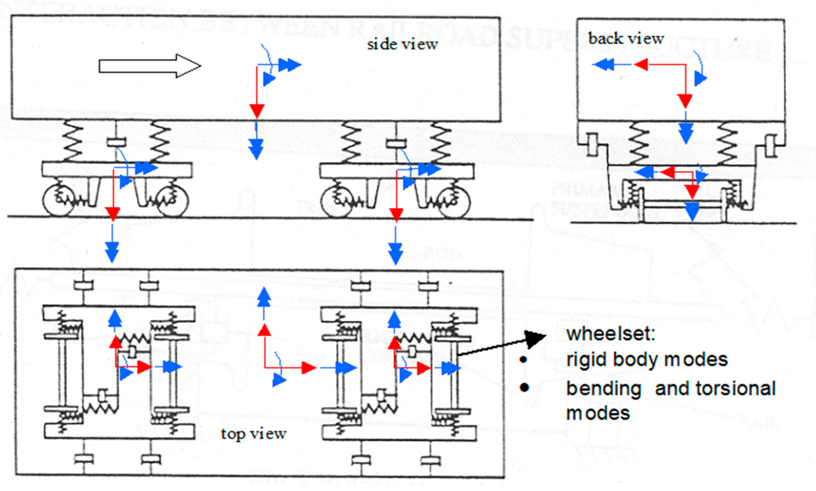
Each car of the train is built as a multibody system, according to the model depicted in Figure 4 and described in references [12,13]. For each vehicle, the carbody, the bogies, and the wheelsets are modeled with six d.o.f. bodies. The following equation) describes the equation of motion of the vehicle model:
where xvi is the vector with the d.o.f. of the i-th car of the train (from 1 to n), [Mvi] is the global mass matrix, [Cvi] is the global damping matrix, and [Kvi] is the global stiffness matrix. Fvi is the vector of contact forces between the rails and the wheels, and Fnli contains terms coming from the non-linear suspension components, such as lateral bump stops and rheological dampers, which are not in any case, key parameters for the present work.
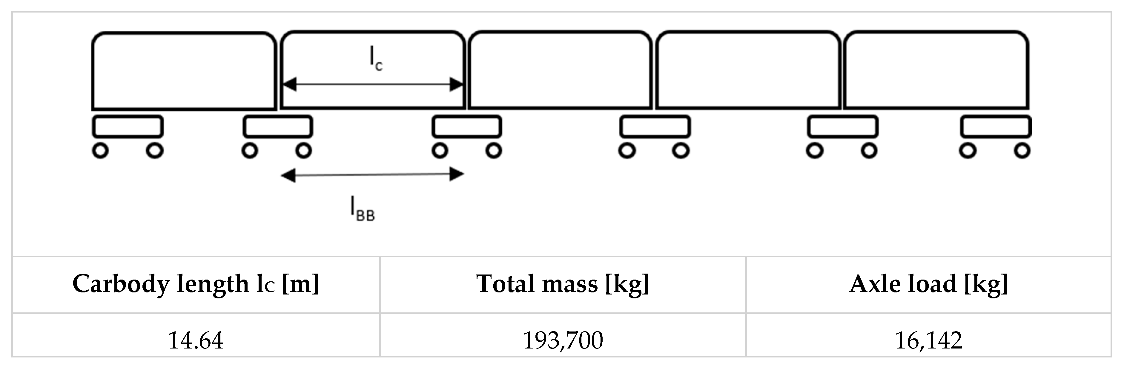
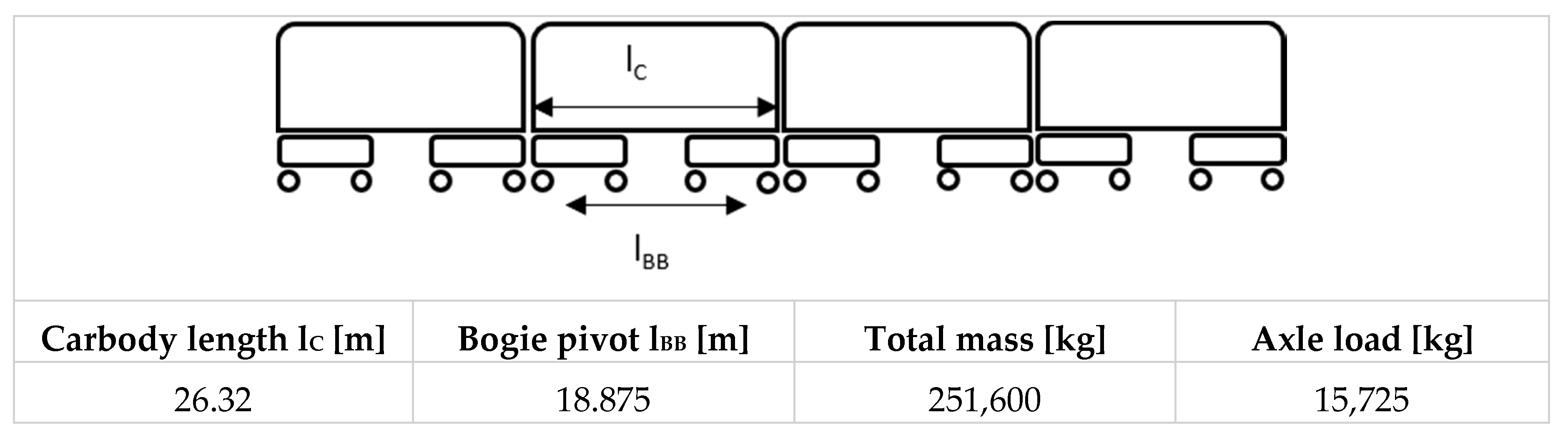
Two different types of trains are considered for the simulations, the first one with bogies shared between adjacent carbodies as in Figure 5 (Italian regional fast train, CSA), and a second one with the standard two-bogies configuration for a single carbody, as shown in Figure 6 (Italian regional train, TSR). The CSA train type consists of five carbodies supported by six bogies, and it is a relatively light train that is used for airport services, whereas the TSR train has a double-deck design, and it is therefore heavier than the CSA train. It is used for regional passenger transport, and it is composed of four carbodies, each supported by two non-shared bogies. The two train models are built with the actual data and properties from the real trains, some of which are reported in Figure 5 and Figure 6.
Both the vertical and lateral dynamics are considered, although for the present application, only the former is involved, since the track is placed in the center of the bridge structure, and the deck torsional motion is not excited.
2.3. Train–Track–Bridge Interaction
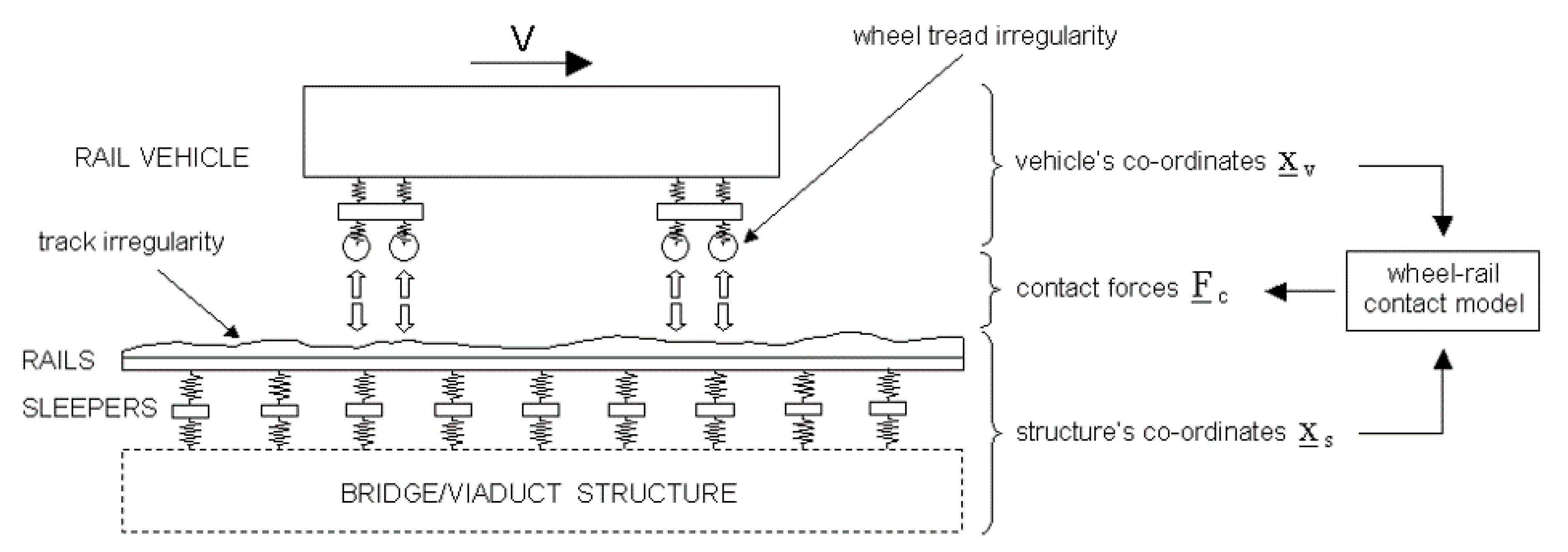
The complete train–track–bridge model is obtained by coupling the bridge and the train models with the expression of the contact forces between the wheelsets and the rails. The complete model is shown in the scheme of Figure 7. The adoption of track irregularity and wheel tread irregularity is optional in the model.
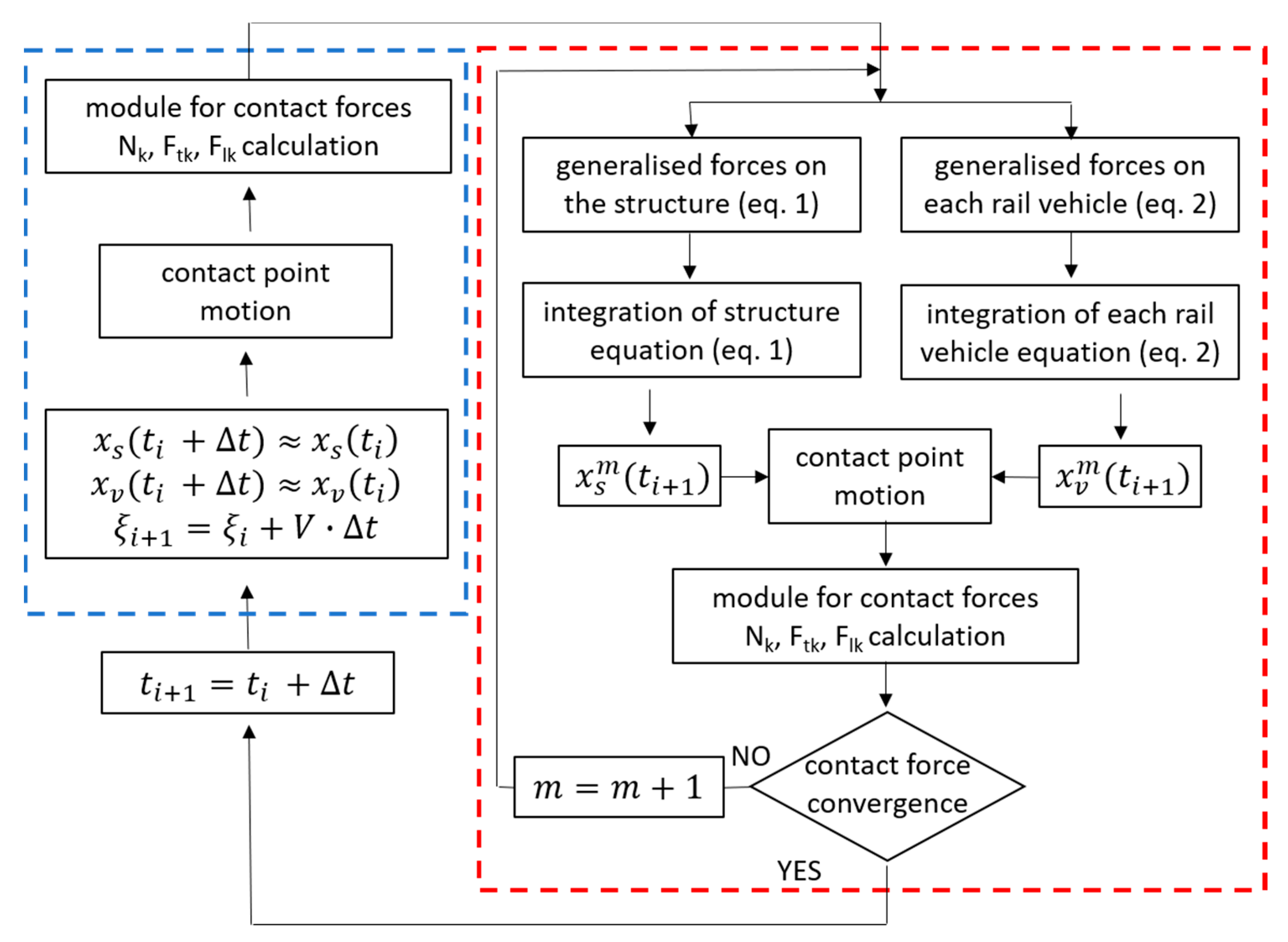
The equations of the motion of the bridge, track, and the superstructure, and of the vehicle are integrated in time, in order to solve the vectors and representing the degrees of freedom of the structure and of the vehicle, respectively. The numerical integration process is described in the flowchart of Figure 8, where ξi represents the position of a wheel along the i-th finite element, Nk, Ftk, and Flk are the normal, tangential, and longitudinal components, respectively, of the contact force on the k-th wheel.
At the beginning of each time step (starting from the blue dashed square on the left in Figure 8) approximations of the displacements of the contact points are calculated, based on the previous step values. A first estimation of the contact forces can then be calculated through the contact force model [12]. Based on these tentative contact force values, the generalized forces on the structure and on the vehicle can be calculated, and the equations of motion can be integrated (red dashed-line square on the right). Once the vectors containing the solution of all the degrees of freedom of the structure and of the vehicle are obtained, the motion of the contact points on the rail and on the wheel, and consequently the contact forces, can be calculated. An iteration loop is begun within the same time step, by integrating the equations of motion again with the new calculated contact forces, until convergence for contact forces is reached. Afterwards, the time step is increased, new approximations are made, and the numerical integration cycle starts again.
3. Plan of the Simulations
For a comprehensive assessment of the feasibility of the drive-by monitoring system, the dynamic response of the two types of trains is analyzed when crossing the four bridge models in different operational conditions. For each bridge/train couple, parameters such as train speed, sensor position, damage severity, and damage location are changed individually, to investigate the impact of each parameter on the performance of the algorithms for damage detection and localization. The last part of the simulations plan is aimed at evaluating possible aspects that may affect the feasibility of the method, such as track irregularity, ballast degradation, and the differences in the track stiffness that the train encounters when entering the bridge.
3.1. Train Speeds
Speeds from 80 km/h to 140 km/h, corresponding to normal traffic conditions of the considered commuter trains, are selected for the analysis.
In the bridge/train interaction, a main excitation source is related to the train axle spacing, determined by the number of vehicles, each vehicle length, bogie spacing, and axle spacing within a bogie. This source of excitation is characterized by a wide spectrum [14,15], which is mainly visible through sensors placed on the track. For sufficiently long trains, the main spectral peaks occur at multiples of the vehicle passing frequency, depending on the ratio between the train velocity and the vehicle length (i.e., v/lc, with lc being indicated in Figure 5 and Figure 6 for the CSA and TSR trains respectively). The vehicle length lc corresponds to the distance between bogies in the case of the CSA train, and to the distance between two pairs of adjacent bogies, in the case of TSR train. A second source of excitation, visible on vehicle accelerations, is the span passing frequency. It is related to the time that is needed for each axle and bogie to cross the bridge, and it is equal to the ratio between the train velocity and the bridge length (i.e., v/lspan). Table 3 reports, for all the considered speeds, the values of the span-passing frequencies and the excitation frequencies related to vehicle lengths. The latter are higher in the case of CSA train than the TSR train, due to the lower lc value. In the considered speed range, all of these frequencies are well below the first mode of vibration of all the bridge model considered. Resonance-like phenomena are therefore not generated due to the span passing frequencies and for the high-resonance bridge #1, whereas bridge natural frequencies may still be excited by multiples of the vehicle passing frequency. This will be verified from the results of numerical simulations.
3.2. Sensor Location on the Train
The best positioning of acceleration sensors on the vehicle depends on several aspects: capability to reveal the defect, signal-to-noise ratio, and effort required for maintenance. The latter aspect is also relevant, since sensors are thought to be used on an operating train fleet. Sensor locations considered in the present analysis are on bogies and wheelsets, since a previous work [5] showed that carbody acceleration signals are not sensitive enough to detect a defect on the bridge. A second issue is related to the location of the sensor along the train. In principle, it can be considered that differences may be found between accelerations at the front and at the rear of the train, since the leading bogies interact with an unperturbed bridge, whereas the middle and rear part of a train find a bridge already excited by the passage of the first part of the train. For this reason, the comparison between accelerations corresponding to the first and fourth bogies are considered in the present analysis. In addition, for each bogie, vertical accelerations corresponding to different positions on the bogie frame are calculated. These positions, regarded as virtual measuring points, are indicated in Figure 9, with numbers from 1 to 4.
For each of the two bogies (i.e., first and fourth of the train), accelerations corresponding to the leading wheelsets are considered. The accelerations at left and right wheels are also calculated, based on the degrees of freedom that are related to the vertical motion of the center of gravity (zw) and roll rotation (ρw) of the wheelset. These measuring points are investigated to evaluate the performances of sensors on axleboxes, which is another feasible position for where acceleration sensors for diagnostic purposes can be placed [16]. Figure 10 shows a scheme of a wheelset, with indications of the degrees of freedom (zw and ρw) adopted for calculation.
The evaluation of the best location for sensors is performed through simulations without track irregularity, to neglect differences in accelerations due to random effects, and to focus only on systematic differences that are related to the dynamic interaction between the train and the defective bridge. Clearly, simulation results show that on straight track with no irregularity, and with a defect covering the entire bridge width, the roll motion is not excited. On the other hand, the effect of the defect on bogie pitch is visible. In the following Section 4, the analysis is therefore focused on the results of vertical acceleration on bogie center of mass zB, bogie frame edges zB1, and zB3 (see Figure 9), and the wheelset center of gravity zw (see Figure 10).
3.3. Damage Severity and Location
Four different damage levels are simulated, with Young’s modulus in the damaged finite element, respectively reduced by −25%, −40%, −55% and −70% with respect to the steel value of 206,000 MPa being assumed as a reference. The defect modeled in this way is intended to be representative of a decrease of flexural stiffness, generated by a loosening of a diagonal element in the truss bridges, or a reduction of the deck section, caused by extensive cracking in the concrete structures [9]. Even if a reduction of Young’s modulus of up to 70% is unlikely, it was still investigated in the sensitivity analysis, to evaluate the trend in accelerations due to damage severity. To investigate if the location of the damage has an influence on the applicability of the algorithms for damage detection, each simulation is repeated for two different damage locations, one with the damage in the middle of the bridge span, and the other with the damaged element located at around one quarter of the bridge span. Table 4 reports the positions of the damaged element for each bridge, made dimensionless by dividing the starting and ending locations of the damaged element by the bridge length.
3.4. Data Processing Techniques
Figure 11 compares the accelerations of the center of gravity of the leading bogie in the case of the damaged bridge (dashed orange line) and of the healthy bridge (continuous blue line). Figure 11a reports the time domain signals, as a function of position along the bridge. To make the diagram layout adoptable for bridges of different span length, and to ease the comparison of results of damage localization between different bridges, the horizontal axis is rescaled into a dimensionless range from 0 to 1, representing respectively, the initial and final sections of the bridge. Figure 11b reports the power spectral density (PSD). The results refer to bridge #2, the TSR train type, a speed of 100 km/h, damage level D40 (i.e., 40% reduction of flexural stiffness). In the time domain signals of Figure 11a, the position of the defective element is highlighted by two vertical red lines. A difference is visible, starting just before the location of the defects, and continuing further after its end. In the PSD of Figure 11b, three main frequency ranges are identifiable:
- a low-frequency range, including the acceleration of the trajectory related to the quasi-static response due to the bridge deflection under the train load. This value depends both on the amplitude of bridge deflection, and on the period for crossing the bridge.
- A second contribution at around 5.5 Hz, corresponding to the first natural frequency of the bridge (which is a bit lowered by the presence of the train mass).
- A third frequency contribution at 46.3 Hz, generated by the wheelsets crossing the sleepers. The latter are equally spaced in all the bridge models developed (lsl = 0.6 m), so that the sleeper passing frequency depends only on the speed of the train v, according to the formula fsl = v/lsl. Since the considered defect is related to deck damage, its presence does not increase the amplitude of the sleeper passing frequency in any of the cases analyzed.
Two different approaches for data-processing are investigated, basically differing in the frequency range taken into account for accelerations. In a first approach (see Section 3.4.1), the acceleration data are low-pass filtered to cancel the dynamic component due to the bridge first mode of vibration. The remaining signal is representative, in terms of acceleration, of the quasi-static deflection of the bridge in response to the moving loads. A second approach (see Section 3.4.2) also considers the first natural frequency of the bridge, as well as other natural frequencies that are related to bogie dynamics (vertical and pitch), if excited. Sleeper passing frequency is excluded from this range of analysis, since for the type of defects considered, it does not contain the relevant information to discern between damaged and healthy bridges.
3.4.1. Quasi-Static Method
The quasi-static method derives from the works presented in [9,10], which are focused on a bridge for road transportation. The method applied in these papers consists of filtering the signals with a moving average filter with a window length that is equal to the period of the first mode of vibration of the bridge, to cancel the dynamic components of the acceleration, and to extract the quasi-static component. The signal obtained for the healthy and damaged bridges are then compared, and the difference between the two signals (hereafter called damage component) is used as an indicator of the presence of structural damage.
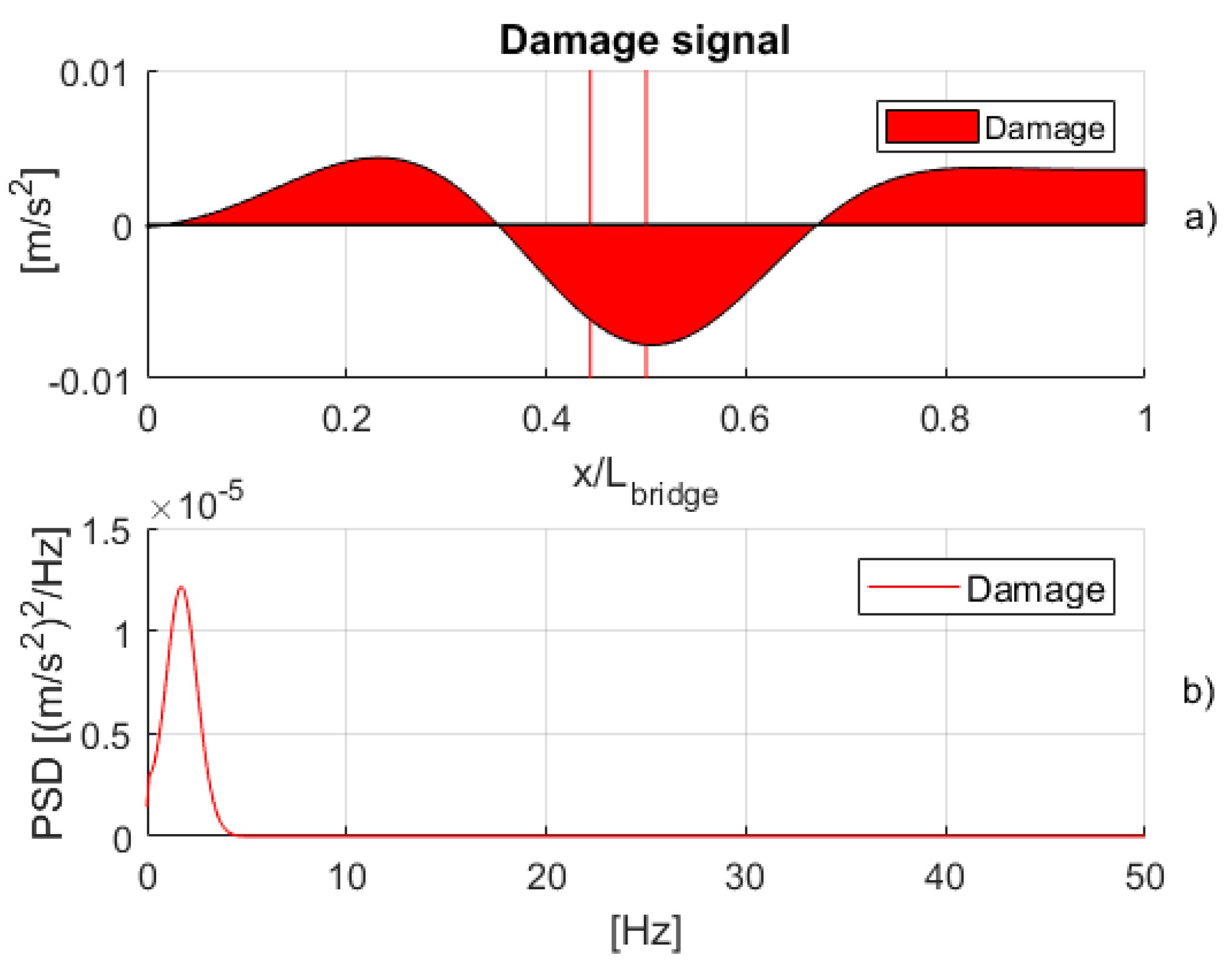
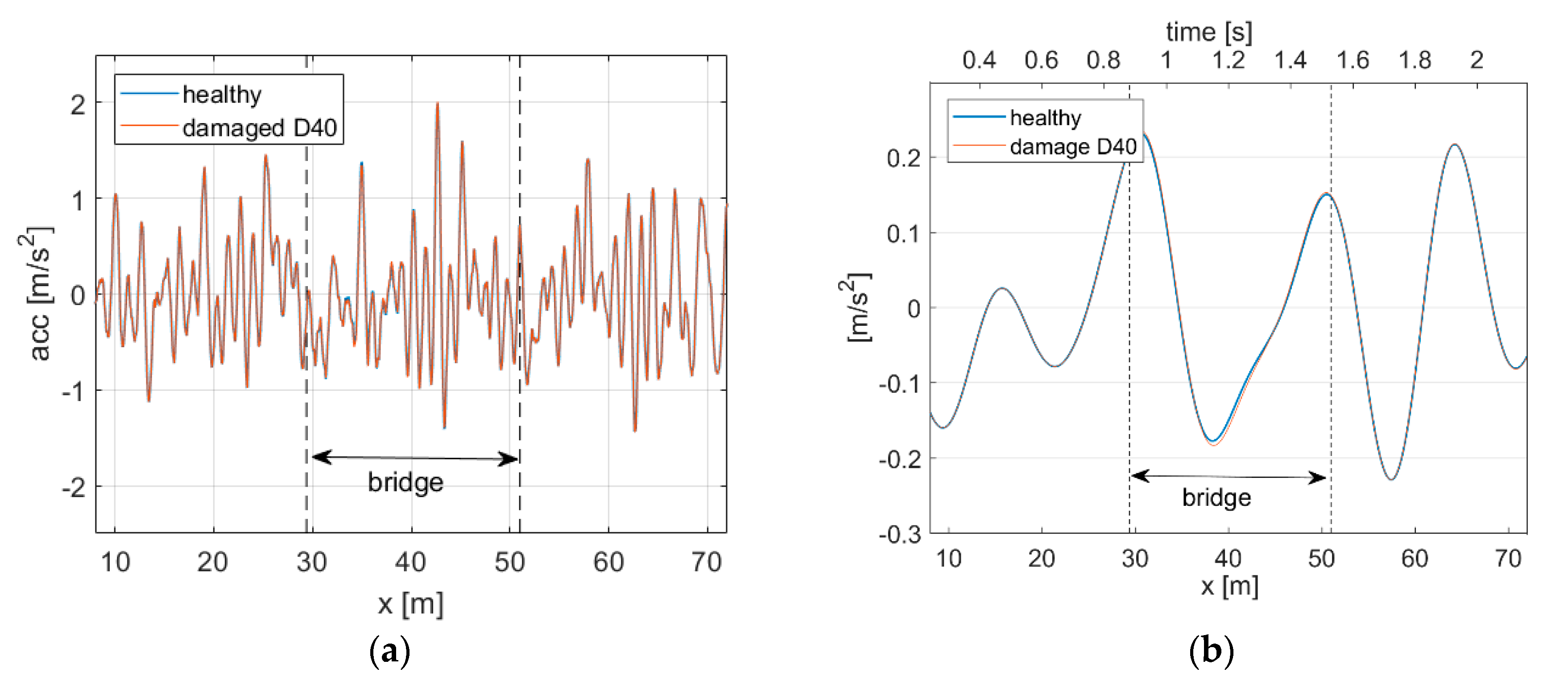
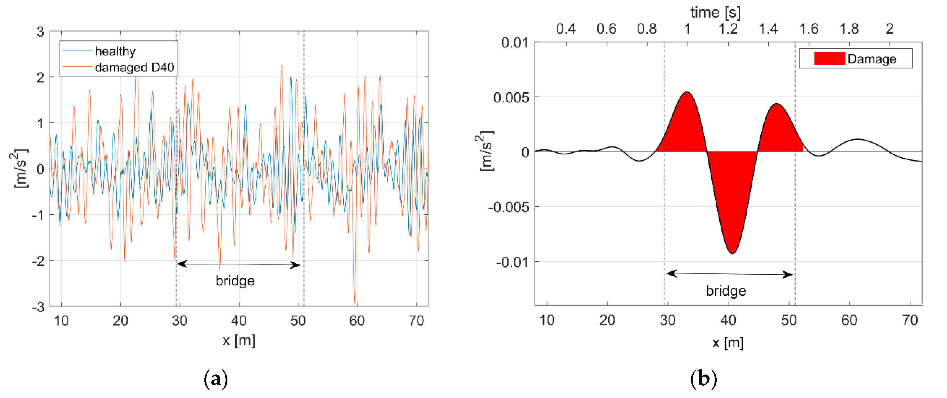
In this work, the same idea is developed, considering the peculiarities of the railway application, mainly consisting in longer vehicle and higher axle loads. Acceleration signals are low-pass filtered with a cut-off frequency depending on the first natural frequency of the bridge, to cancel the dynamic component due to bridge vibration. Figure 12 shows the accelerations of the damaged and healthy bridges after the low-pass filtering. Only the quasi-static component due to bridge deflection under the moving load is still present, with the highest acceleration levels corresponding to the damaged bridge. The difference of the two signals, representing the damage component, is filled with color in Figure 12a.
To identify the location of the damage, the acceleration corresponding to the healthy signal is subtracted from the acceleration acquired on the damaged bridge, obtaining the damage component. Figure 13 shows the damage component corresponding to the signals of Figure 12, which shows a maximum at position 0.505. This value is situated 0.7 m after the midpoint of the range [0.444; 0.5], in which the finite element with reduced Young modulus is located. The method is therefore sufficiently accurate for indicating the actual location of the damage.
A fifth-order butterworth numerical filter is adopted. The cut-off frequency is a key parameter for the application of the algorithm, and it was set as a trade-off between the need of accuracy in damage localization, and the need of a high level of the damage component. The more that the signal is filtered, the better accuracy in positioning is obtained, but the acceleration level of the damage component is lowered. The cut-off frequency is obtained by reducing the bridge first natural frequency by a factor kcut: fcut = kcut × fbridge. kcut value was set between 0.5 and 0.7, based on simulation results. For very short bridges with natural frequencies higher than 10 Hz, such as bridge number 1 (Table 1), the cut off frequency was upper-limited at 5 Hz, in order to filter natural frequencies that are related to the bogie vertical and pitch dynamics.
3.4.2. Root Mean Square (RMS) on the Moving Window
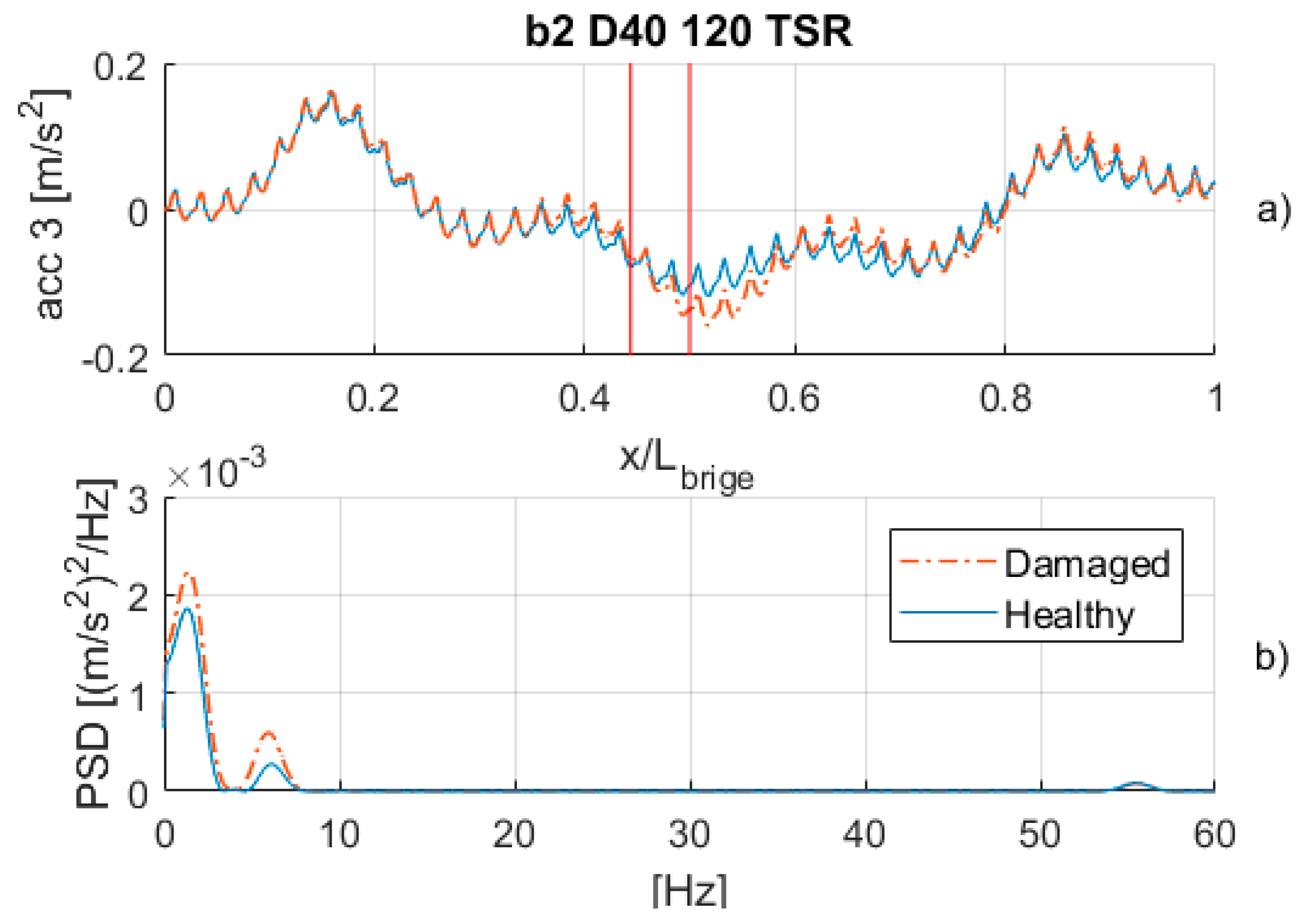
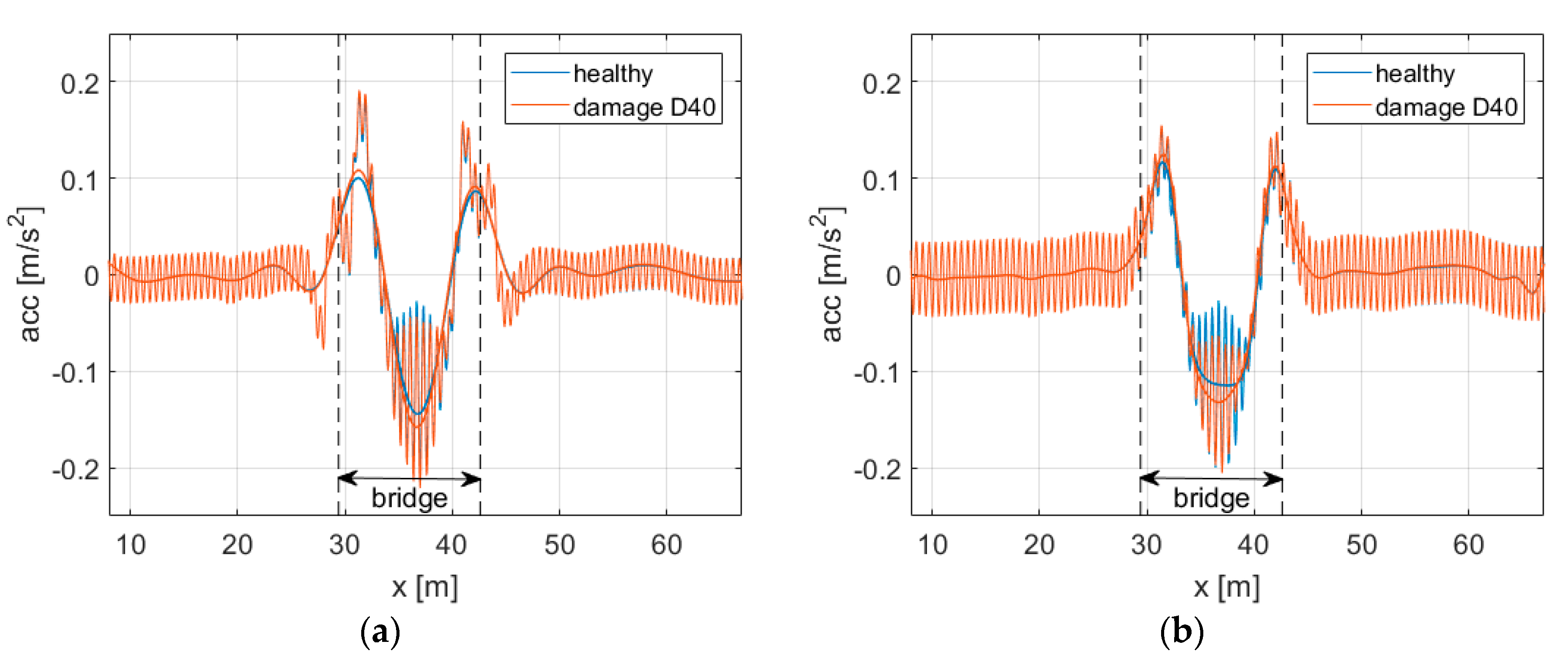
The second approach that is proposed is intended to look for an effect on the dynamic response of the vehicle, caused by the presence of damage on the bridge, seen as a local disturbance. In principle, indeed, the presence of a defective section can generate a variation in the amplitudes of frequency components of bogie andaxlebox accelerations, not only in the quasi-static frequency range, but also in the natural frequency related to bogie motion, and in the frequency related to the bridge first flexural mode, when excited. Figure 14 shows the accelerations of point number 3 (see Figure 9) of the leading bogie, corresponding to bridge #2, train (TSR), damage entity (D40), with a train speed of 120 km/h. In the time signals, the difference in the acceleration recorded for the healthy and damage bridge starts slightly before the faulty section and continues several meters after it. In the frequency domain, an increase in the PSD component related to the bridge natural frequency is observed for the damaged bridge.
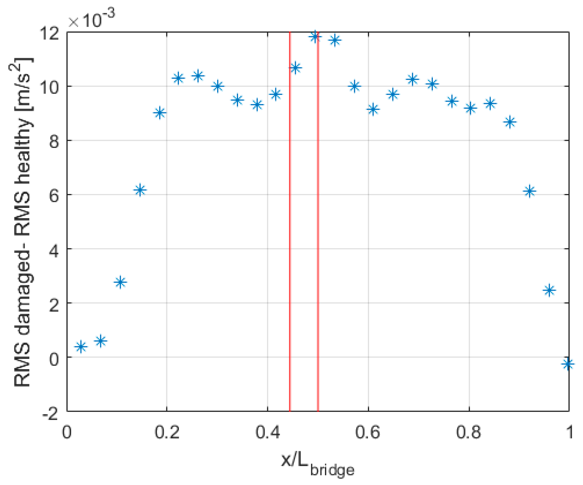
To catch the variations in the dynamic behavior of the system, and to precisely localize the position where this variation is maximum, an RMS with a moving average window is performed with length T = 0.4 s, and a high overlap level of 95%. (The time-based window length of 0.4 s corresponds to 13 m at 120 km/h). Before calculating the RMS, signals are filtered with a cut-off frequency of 30 Hz, since no relevant differences were detected in the acceleration peaks that are related to the wheelset crossing of the sleepers. RMS corresponding to the healthy and damage conditions are then subtracted, and the RMS damage component is obtained. The result of the analysis is reported in Figure 15, highlighting that the maximum of the RMS damage component corresponds to the location of the defect.
3.5. Effects of Track Irregularities
In real operating conditions, the track profile is affected by deviations from its nominal geometry, which are described as the vertical and lateral alignments of each rail. The vertical track irregularity, also named the “longitudinal level” in current terminology, is the one that is relevant for the present work. It is simulated to include wavelengths from 100 m down to 1 m, corresponding to time frequencies from 0.39 Hz to 39 Hz at a maximum speed of 140 km/h. The irregularity profile is characterized by an RMS level that is equal to 2.1 mm in the wavelength range from 1 to 100 m, and an RMS that is equal to 0.8 mm in the wavelength range from 3 to 25 m. (The latter is the wavelength range that is adopted by the Italian infrastructure manager to qualify longitudinal irregularity). The peak-to-peak amplitude of the profile is equal to 8.2 mm.
A first consequence due to vertical track irregularity is the excitation of the modes of vibration of the vehicles in the above-mentioned frequency range, namely the carbody bounce and pitch (usually below 2 Hz), and the bogie bounce and pitch (usually between 4 and 11 Hz). These frequencies fall within the ranges of analysis of the two methods that are described in Section 3.3 and Section 3.4. In particular, the low-pass filter of the quasi-static method removes from the analysis only the natural frequencies related to the bogie, whereas both the carbody and bogie natural frequencies are included in the range that is related to RMS analysis. The background acceleration level is increased, hardening the comparison of the signals generated on the train crossing a healthy bridge and a defective bridge.
The damage detection algorithms rely on the comparison of the acquired signal against a reference condition, so that the evolution of the track irregularity between subsequent data acquisitions is another effect that could affect the feasibility of the method. Track geometry degradation in railway lines can generate long wavelengths, usually due to ground settling, and shorter wavelengths, due to ballast settling. The former is a slow process, which is more likely to happen in the track sections on ground before and after the bridge, and not on the bridge structure. It can be monitored by performing a trend analysis of the acquired data, and updating the reference signal constantly. Short wavelength irregularities can evolve more quickly, and they may occur also on a bridge track section, even if in a mitigated way, due to the fact that the ballast is contained within the deck side walls, and its settling is partially prevented. To evaluate the effect of an evolution of track irregularity on the bridge in the wavelengths related to ballast degradation, the algorithms for damage detection were run on accelerations obtained with different irregularity profiles for the healthy bridge and for the damaged bridge. The reference irregularity already mentioned (RMS 2.1 mm, 1–100 m range) was adopted for the healthy bridge simulation. This profile was then modified in the wavelength range from 1 to 6 m, by doubling the spectral amplitudes and randomly shifting their phases, and adopting for the simulation of the damaged bridge. The modified wavelengths, corresponding to time frequencies ranging from 3.7 to 39 Hz in the 80 to 140 km/h speed range considered in this work, influence the level of excitation of the bogie natural frequencies. The consequences of this process on the results of the damage detection algorithms are described in the next section.
A last effect that is investigated is related to the possible variation of the track vertical stiffness encountered by the train when entering the bridge. Since the ballast on the bridge is directly placed on the deck instead than on the soil subgrade, and the ballast layer normally has a lower depth on the bridge, the train may be subjected to an increase of vertical track stiffness. To qualitatively simulate the phenomenon, a dedicated simulation was carried out for the short bridge #1, by building a FEM model with a reduction of 25% of the vertical stiffness of the ballast in the straight track before and after the bridge.
4. Simulation Results
Simulation results without track irregularity showed that a reduction of flexural stiffness on a bridge element marginally affects the dynamic response of the train in terms of the excitation of vehicle natural frequencies, and the main differences in the vehicle accelerations corresponding to the healthy and damaged bridges are related to the quasi-static response due to the bridge deflection under the train load. For this reason, the acceleration levels of the damage signal obtained through the quasi-static and RMS algorithms are comparable for most of the simulated cases. For some cases in which the bridge natural frequency becomes more visible for increasing speeds, the RMS method shows a higher level of acceleration in the damage signal. It must be considered, though, that the frequency component of acceleration that is related to the bridge natural frequency becomes almost irrelevant in simulations with track irregularity, in which the natural frequencies of the bogie are excited, and the background acceleration level is increased. Moreover, since a possible degradation of track irregularity on the bridge (e.g., ballast degradation) alters the dynamic response of the vehicle in a wide range included in the RMS analysis, the RMS algorithm is less robust with respect to an evolution of track irregularity, when compared to the quasi-static algorithm. For these reasons, the quasi-static algorithm seems to be preferable, and only its results are presented in detail in the following section.
4.1. Best Sensor Positioning
The quasi-static algorithm for damage identification was run for vertical accelerations of the first and fourth bogies and vertical accelerations of their leading wheelsets, for all speeds, damage levels, damage locations, bridge models, and train types. A damage localization error index (DLE) is introduced to quantify the accuracy of damage localization that is achievable with sensors installed in different positions on the train. This index averages the differences between the predicted damage location and the actual position of the “damaged” finite element for all the results from every bridge model, every damage level, and every considered speed. DLE is defined in the following equation:
in which xbegin and xend are the starting and ending positions of the defective finite element, and n is the number of simulation cases (i.e., n = 64, having four bridge models, four damage levels, and four speeds). Table 5 and Table 6 report the DLE results for all the measuring point considered, for the damage at midspan and at a quarter of the span. In the case of measuring points on bogie number 1 and 4, the label “central” indicates the position of the bogie center of gravity, whereas “Mp1” and “Mp3” are the measuring points numbered 1 and 3 in Figure 9. As for the wheelset, the label “wheelset 1b1” refers to the leading wheelset of the first bogie, whereas the label “wheelset 1b4” refers to the leading wheelset of the fourth bogie. The results in Table 5 correspond to the CSA train, and those of Table 6 to the TSR train. The measuring point that yields the smallest DLE value can be considered as the optimal measuring point location.
Indications given by the two train types are consistent with the fact that a sensor placed at the front of the train can better identify the damage location, when compared to sensors that are placed in the middle of the train. The DLE indices corresponding to the column ‘Bogie 1’ are indeed always lower than the corresponding values in ‘Bogie 4’, as well as the DLE values in column ‘Wheelset 1b1’ are always lower than the corresponding values in ‘Wheelset 1b4’. The optimal measuring point should therefore be found on the first bogie or on its corresponding wheelsets, and the next appraisals in this paper will neglect the results from bogie 4 and its wheelset. This result is remarkably different from the one that is obtained in resonant bridges, in which the trailing bogies give stronger indications for the presence of a defect, with the signal amplitude becoming higher and higher during the train passage [7]. In the case here investigated, in which the algorithm seeks for alteration in the quasi-static response, differences in accelerations generated by a defect can be identified more precisely on the leading bogie, since it interacts with an unperturbed bridge.
To evaluate the best sensor placement between the bogie and the axlebox, column ‘Bogie 1’ is compared to column ‘Wheelset 1b1’. The lowest value for the DLE index can be found in the column ‘Bogie 1’ in most of the cases, so that the sensor placement on the bogie must be preferred. Another reason supports this choice: thanks to the filtering action from the primary suspension, in the higher frequency range, the acceleration levels potentially measured on the bogie frame are much lower than on the axleboxes. Therefore, a more sensitive accelerometer with lower full-scale can be fitted on the bogie, without saturation. This is fundamental in applications such the one considered here, in which the differences to be discerned in the accelerations are very small.
Finally, DLE indices are smaller for the CSA train type for each measuring point location on the first bogie. However, acceleration levels of the damage component corresponding to the two trains are not always higher in the CSA case, so that no ultimate conclusions can be drawn about the performance of one train type, with inter-carbody bogies, with respect to the other. On the practical side, this is a positive outcome, since no specific train configuration is required.
4.2. Acceleration Level and Damage Localization
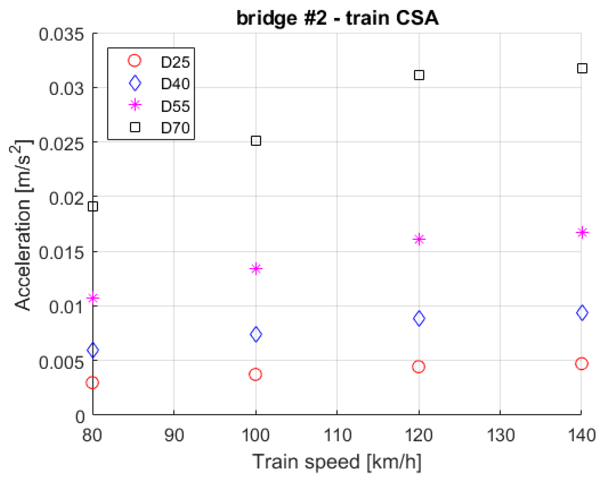
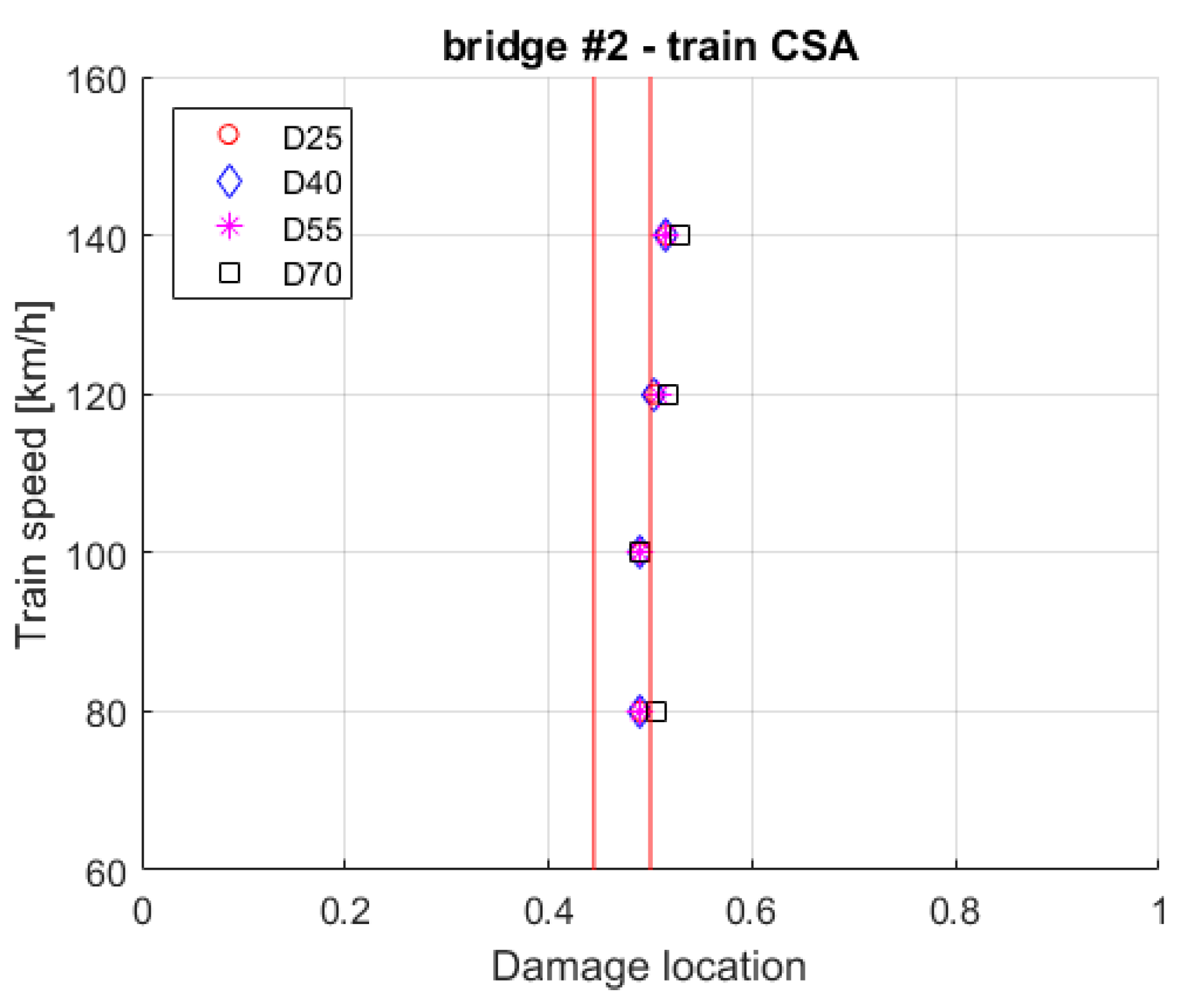
As already mentioned, one of the more challenging issues of the drive-by method is related to the small differences in accelerations to be detected, to discern between a case of a healthy bridge from an unhealthy one. This leads to problems of a low signal-to-noise ratio, and the sensitivity of the accelerometers in the lowest frequency range. To comment on the feasibility of this method, this section shows the results of the acceleration levels of the damage component, which should be as high as possible. Figure 16 reports the influence of the train speed and of the damage entity on the damage component of the acceleration. These exemplary results refer to bridge #2 and to CSA train type, results from the TSR train being similar in order of magnitude. The damage is located at mid-span.
As obviously expected, the magnitude of the damage component increases both with speed and damage level, with high damage levels being more speed-sensitive. The highest speed seems to be the best perspective for damage identification; however, this aspect may contrast with the need of the accuracy of damage localization, as shown in Figure 17, reporting the influence of damage level and the train speed on the accuracy of damage localization. The vertical red lines in the figure define the non-dimensional positions of the starting and ending point of the damaged finite element. It can be observed that the algorithm correctly localizes the damage within this range for lower speeds, whereas at a speed of 140 km/h, the damage is located a bit further the actual defect (non-dimensional location 0.516, with an absolute error corresponding to less than 1 m). When increasing the train speed, a delay in the damage localization appears. This trend is representative of all the other bridge models, measuring point locations on trains and damage located at a quarter of the span length.
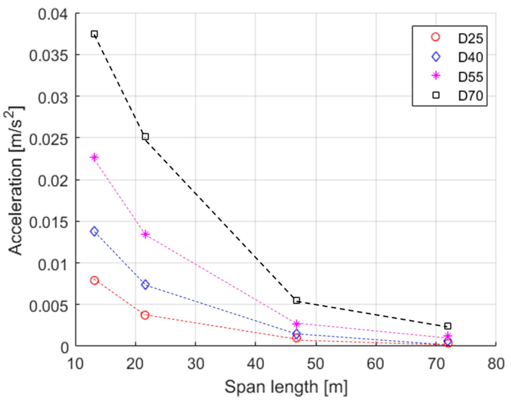
Figure 18 shows the relation between the magnitude of the damage component and the span length of the bridge. These results are obtained from simulations with all the bridge models and damage located at midspan, considering all damage levels. The results corresponding to CSA train type at 100 km/h are shown, with similar results being obtained for other speeds and the TSR train.
The highest magnitudes of the damage signals are obtained for the shortest span lengths. This result is consistent with the fact that, even if the bridges with the longest span are subjected to higher displacements due to the simultaneous loading of more than one bogie, shorter bridges are crossed in a shorter time, resulting in higher accelerations on the bogie. Assuming that the acceleration difference between the damaged and healthy bridges is proportional to the peak value, the effect of a defect in the bridge is therefore more visible in shorter bridges.
To analyze the influence of the span length on the accuracy of the damage localization, the DLE index was calculated, averaging over all of the speeds for one bridge model and one damage level. Results showed that the accuracy of the damage localization technique is higher for the shorter span length, so there is no conflict in this case between the two prerequisites of accuracy and acceleration amplitude.
4.3. Track Irregularities
Simulations with track irregularity were carried out to assess the feasibility of the damage detection method when the vehicle modes of vibration are consistently excited, and the background acceleration level is increased. Figure 19a shows the vertical accelerations of the leading bogie of the TSR train, obtained with the first irregularity profile defined in Section 3.5 (i.e., RMS 2.1 mm in the 1–100 m wavelength range), for the case of bridge #2 (damage D40 and healthy), and a train speed of 120 km/h. Figure 19b shows the same signals filtered with a cut-off frequency of 2.95 Hz (i.e., 0.5 × fbridge). In the figure, the distance covered by the train is reported in the bottom x-axis [m], and the corresponding time [s] in the top x-axis. Two dashed vertical lines report the bridge position, and the sections just before and after the bridge correspond to the ballasted track.
The variability of the filtered acceleration due to track irregularity (Figure 19b) is of the same order of amplitude of the acceleration related to bridge crossing (see Figure 11 and Figure 12), and one order of magnitude higher than the difference between accelerations of the healthy and the damaged bridge. This means that the damage identification procedure would be definitely affected by an evolution of long waves irregularities. It is therefore fundamental that these irregularities, which evolve anyway in a slow process, are constantly monitored, and that the reference condition is updated.
The carbody bounce and pitch natural frequencies, being usually lower than 2 Hz, and therefore lower than the cut-off frequency, are not filtered in the quasi-static procedure. For the TSR train model, these frequencies are equal, respectively, to 0.84 Hz and 1.22 Hz. Even if in the corresponding mode shapes the contribution of the bogie vertical motion is not negligible (15% of the carbody vertical motion for the bounce mode), the corresponding natural frequencies are not visible in Figure 19b to an extent which may affect the feasibility of the method. This is mainly due to the high non-dimensional dampings, which are equal to 22% for the carbody bounce and 32.9% for the carbody pitch, and it is an aspect in favor of the feasibility of the method.
A persistence in the capability to identify the damage is confirmed when the healthy and the damaged bridge are simulated with different irregularities, to reproduce from a qualitative point of view the variation of short wavelenghts that may be generated by ballast degradation. The irregularity adopted for the healthy bridge (same as in Figure 19) was modified in the wavelength range from 1 to 6 m, by doubling the amplitudes and randomly shifting the phases, and then adopted for the simulation of the damaged bridge. Figure 20a reports the vertical accelerations of the leading bogie corresponding to the healthy and damaged bridge, whose differences are due to the different irregularity profiles. Figure 20b reports the damage signal, obtained as the difference of the filtered accelerations. The results of damage identification are positive and similar to the case with no irregularity, since the variations in vertical accelerations due to the change of irregularity profile are filtered in the quasi-static algorithm.
Finally a modified finite element model was built by adopting, for the ballast on track sections out of the bridge, a vertical stiffness (kz = 0.4540 × 10⁸ N/m) that was lower than the one that was adopted on the bridge (kz = 0.6040 × 10⁸ N/m). This was aimed at simulating the increase of ballast stiffness, which may be found when the train enters the bridge, due to the lower height of the ballast subgrade and to the absence of soil. Figure 21a shows the results of the leading bogie accelerations corresponding to the damaged and healthy bridge in the case of ballast with modified stiffness, whereas Figure 21b shows the same signals in the reference case with homogeneous ballast stiffness. The results refer to the short, high-resonance bridge #1, TSR train, with a speed of 120 km/h. Simulations with no track irregularity are considered, in order to clearly detect only the effect that is related to the difference in the track stiffness encountered by the train entering the bridge. In the figures, the low-pass filtered signals are superimposed to the full-range accelerations with continuous lines. Even if the presence of the abrupt stiffness variation at the beginning of the bridge generates an excitation of the vehicle natural frequencies and an elongation of accelerations in Figure 21a, in the filtered signals the difference with accelerations of the reference case in Figure 21b is attenuated. The damage components generated by the difference of the filtered signals (healthy-damages) of Figure 21a andb are not significantly different in the two cases.
4.4. Further Research Required
The results reported in the previous section confirm that the drive-by method shows, when relying on numerical simulations, good performances in damage localization, and the highest amplitudes of the damage signal in the case of short bridges. Nevertheless, a few challenging items must be tackled for applications in a real railway environment, before this method can be tested in practice:
- the difference between the accelerations generated on the train by healthy and unhealthy structures is in the order of 10−2 m/s2 or even 10−3 m/s2, which leads to potential operational difficulties [5]. The required sensitivity indeed conflicts with the full-scale range that is needed for the acceleration sensors placed on the wheelsets, whereas this issue is less severe for sensors placed on the bogie frame. To overcome this drawback, high sensitive accelerometers should be placed on the mechanical suspensions (e.g., silicon pad or rubber layers), to reduce acceleration peak values by filtering all of the frequencies that are outside the range of interest. Such a configuration has already been adopted for selecting a specific frequency range in acceleration measurements on the axlebox [17].
- The method relies on the comparison between the current data acquisition and a reference “healthy” signal, so that the actual position of the train along the bridge must be known. A first solution may be to place a transponder at the beginning and at the end of the bridge, so that the actual position of the measuring point can be calculated at each time, based on the train speed value. A second solution may be the adoption of a geo-localization system for the train, based on high-performance GPS and odometry, which would allow for correlating acceleration data with the actual position of the train at the instant that they were acquired. This system is being currently developed in Europe for rolling-stock based diagnostics of the railway infrastructure [16,18].
Further investigation will also consider the development of a more refined bridge model, where a defect that is closer to reality can be introduced. This would allow for the quantification of the damage extent, which in this work has been simply considered as a stiffness reduction to perform a sensitivity analysis. Finally, it should be considered that deck torsion that associated with a left/right asymmetry of the defect calls for the consideration of the roll motion of train’s vehicle as well.
5. Conclusions
The paper analyzed the feasibility of a drive-by damage detection method for railway bridges, based on acceleration signals measured on-board the train. The analysis is carried out by numerical simulations of the train–track–bridge interaction, comparing different scenarios with several bridge span lengths, damage levels, damage positions, train speeds, and typologies of bogie arrangement. The identification of a defect in the bridge is carried out by comparison between the signal measured on the train crossing the damaged bridge, and a reference signal corresponding the healthy structure.
Two main criteria are considered to analyze the feasibility of the proposed technique: the magnitude of the acceleration to be measured to discern between a healthy and a damage structure, (i.e., the so-called damage component), and the accuracy of the damage localization. The method proved to be in principle applicable to the velocity range that is typical of a commuter train, with a rather good accuracy in localizing the defect. However, the damage component to be measured is in the order of 10−2 m/s2 or even 10−3 m/s2, which is an issue to be considered for implementation in a real railway environment, where track irregularities can decrease the signal-to-noise ratio.
The acceleration measured on the leading bogie is the most appropriate for damage detection, and the algorithm analyzing the quasi-static response of the bridge shows in general a better performance, allowing a more accurate localization of the damage and a lower sensitivity of the results to an evolution of track irregularity. The highest values of damage components are obtained for the shortest bridges. The damage component increases with train speeds, in the range up to 140 km/h, and with the damage level, whereas the best localization accuracy is obtained for lower train speeds and lower damage levels. This might result in a conflict between the two prerequisites.
Further investigations are needed before that the method can be tested in practice. The major one is related to the possibility of installing high-sensitive accelerometers on the train bogie, with the adoption of mechanical suspensions (i.e., silicon or rubber layers) to filter the frequencies out of the range of interest, and to consequently reduce the full-scale range that is required for the sensors.
Author Contributions
The software used was developed internally at Department of Mechanics of Politecnico di Milano. It is named ADTRES. A.C. supervised all the works and drove the implementation of all the numerical models. M.C. developed the algorithms for damage identification, and performed the analysis related to track irregularities. T.P. performed the simulations without track irregularities and the data analysis, as part of his Master Thesis at Polimi. The paper writing was mainly carried out by M.C. and A.C.
Funding
This research received no external funding.
Conflicts of Interest
The authors declare no conflict of interest.
References
- Vagnoli, M.; Remenyte-Prescott, R.; Andrews, J. Railway bridge structural health monitoring and fault detection: State-of-the-art methods and future challenges. Struct. Health Monit. 2018, 17, 971–1007. [Google Scholar] [CrossRef]
- Leander, J.; Andersson, A.; Karoumi, R. Monitoring and enhanced fatigue evaluation of a steel railway bridge. Eng. Struct. 2010, 32, 854–863. [Google Scholar] [CrossRef]
- Siriwardane, S.C. Vibration measurement-based simple technique for damage detection of truss bridges: A case study. Case Stud. Eng. Fail. Anal. 2015, 4, 50–58. [Google Scholar] [CrossRef] [Green Version]
- Bowe, C.; Quirke, P.; Cantero, D.; Obrien, E.J. Drive-by structural health monitoring of railway bridges using train-mounted accelerometers. In Proceedings of the COMPDYN 2015—5th ECCOMAS Thematic Conference on Computational Methods in Structural Dynamics and Earthquake Engineering, Crete Island, Greece, 25–27 May 2015; pp. 1652–1663. [Google Scholar]
- Amerio, L.; Carnevale, M.; Collina, A. Damage detection in railway bridges by means of train on-board sensors: A perspective option. In Dynamics of Vehicles on Roads and Tracks, Proceedings of the 25th International Symposium on Dynamics of Vehicles on Roads and Tracks (IAVSD 2017), Rockhampton, Queensland, Australia, 14–18 August 2017; CRC Press-Taylor & Francis Group: Boca Raton, FL, USA, 2017. [Google Scholar]
- Keenahan, J.C.; OBrien, E.J. Drive-by damage detection with a TSD and time-shifted curvature. J. Civ. Struct. Health Monit. 2018, 8, 383–394. [Google Scholar] [CrossRef]
- Somaschini, C.; Matsuoka, K.; Collina, A. Experimental analysis of a composite bridge under high-speed train passages. Procedia Eng. 2017, 199, 3071–3076. [Google Scholar] [CrossRef]
- Bruni, S.; Collina, A.; Corradi, R.; Diana, G. Numerical simulation of train-track-structure interaction for high speed railway systems. In Proceedings of the IABSE Symposium—Antwerp 2003, Antwerp, Belgium, 27–29 August 2003. [Google Scholar]
- González, A.; Hester, D. An investigation into the acceleration response of a damaged beam-type structure to a moving force. J. Sound Vib. 2013, 332, 3201–3217. [Google Scholar] [CrossRef] [Green Version]
- González, A.; Hester, D. A bridge-monitoring tool based on bridge and vehicle accelerations. Struct. Infrastruct. Eng. 2015, 11, 619–637. [Google Scholar] [CrossRef]
- Zhan, J.W.; Xia, H.; Chen, S.Y.; De Roeck, G. Structural damage identification for railway bridges based on train-induced bridge responses and sensitivity analysis. J. Sound Vib. 2011, 330, 757–770. [Google Scholar] [CrossRef]
- Di Gialleonardo, E.; Braghin, F.; Bruni, S. The influence of track modelling options on the simulation of rail vehicle dynamics. J. Sound Vib. 2012, 331, 4246–4258. [Google Scholar] [CrossRef]
- Bruni, S.; Collina, A.; Diana, G.; Vanolo, P. Lateral dynamics of a railway vehicle in tangent track and curve: Tests and simulation. Veh. Syst. Dyn. 2000, 33, 464–477. [Google Scholar]
- Milne, D.R.M.; Le Pen, L.M.; Thompson, D.J.; Powrie, W. Properties of train load frequencies and their applications. J. Sound Vib. 2017, 397, 123–140. [Google Scholar] [CrossRef]
- Sheng, X.; Jones, C.J.C.; Thompson, D.J. A theoretical study on the influence of the track on train-induced ground vibration. J. Sound Vib. 2004, 272, 909–936. [Google Scholar] [CrossRef]
- Cangioli, F.; Carnevale, M.; Chatterton, S.; De Rosa, A.; Mazzola, L. Experimental results on condition monitoring of railway infrastructure and rolling stock. In Proceedings of the First World Congress on Condition Monitoring 2017 (WCCM 2017), London, UK, 13–16 June 2017. [Google Scholar]
- Costa, A.; Milani, D.; Resta, F.; Tomasini, G. Wireless sensor node for detection of freight train derailment. In Proceedings of the SPIE 2016—The International Society for Optical Engineering, Las Vegas, NV, USA, 20 April 2016; Volume 9803. Art. no. 98034W. [Google Scholar] [CrossRef]
- Carnevale, M.; Collina, A.; Palmiotto, M. Condition monitoring of railway overhead lines: Correlation between geometrical parameters and performance parameters. In Proceedings of the First World Congress on Condition Monitoring 2017 (WCCM 2017), London, UK, 13–16 June 2017. [Google Scholar]
Figure 1.
Rail model on bridge beam elements (side view).

Figure 2.
Nodes in a bridge section (transversal section).

Figure 3.
Flexural stiffnesses EI22 of the four bridge models, as a function of span length.

Figure 4.
Train model.

Figure 5.
CSA train data.

Figure 6.
TSR train data.

Figure 7.
Complete train–track–bridge interaction model.

Figure 8.
Flowchart representing the numerical integration process [8].
Figure 8.
Flowchart representing the numerical integration process [8].

Figure 9.
Bogie frame structure. Degrees of freedom adopted for the evaluation of vertical accelerations at points from 1 to 4.
Figure 9.
Bogie frame structure. Degrees of freedom adopted for the evaluation of vertical accelerations at points from 1 to 4.

Figure 10.
Wheelset structure. Degrees of freedom adopted for the evaluation of vertical accelerations at points 1 and 2.
Figure 10.
Wheelset structure. Degrees of freedom adopted for the evaluation of vertical accelerations at points 1 and 2.

Figure 11.
Comparison between accelerations of bogie center of gravity, resulting from the damaged and healthy bridges. Bridge type #2, TSR train type, speed 100 km/h, damage level D40. (a) Raw signals. (b) Power spectral density.
Figure 11.
Comparison between accelerations of bogie center of gravity, resulting from the damaged and healthy bridges. Bridge type #2, TSR train type, speed 100 km/h, damage level D40. (a) Raw signals. (b) Power spectral density.

Figure 12.
Acceleration of damaged and healthy bridges after low-pass filtering. (a) Low-pass filtered signals. (b) Power spectral density of filtered signals.
Figure 12.
Acceleration of damaged and healthy bridges after low-pass filtering. (a) Low-pass filtered signals. (b) Power spectral density of filtered signals.

Figure 13.
Damage signal with its frequency spectrum. (a) Damage component. (b) Power spectral density.
Figure 13.
Damage signal with its frequency spectrum. (a) Damage component. (b) Power spectral density.

Figure 14.
Comparison between bogie accelerations resulting from the damaged and healthy bridges. Bridge type #2, TSR train type, speed 120 km/h, damage level D40. (a) Time signals. (b) Power spectral density.
Figure 14.
Comparison between bogie accelerations resulting from the damaged and healthy bridges. Bridge type #2, TSR train type, speed 120 km/h, damage level D40. (a) Time signals. (b) Power spectral density.

Figure 15.
Damage signal obtained through the algorithm calculating RMS on the moving window.

Figure 16.
Acceleration magnitude of the damage component. Train CSA type, bridge #2, damage located at mid-span.
Figure 16.
Acceleration magnitude of the damage component. Train CSA type, bridge #2, damage located at mid-span.

Figure 17.
Damage localization dependence on speed and damage entity. Train CSA type, bridge #2, damage located at the mid-span.
Figure 17.
Damage localization dependence on speed and damage entity. Train CSA type, bridge #2, damage located at the mid-span.

Figure 18.
Dependence of damage component on span length. CSA train at 100 km/h, damage located at the midspan.
Figure 18.
Dependence of damage component on span length. CSA train at 100 km/h, damage located at the midspan.

Figure 19.
Accelerations of the leading bogie in simulations with track irregularity. TSR train, train speed 120 km/h. (a) Full-spectrum signal. (b) Low-pass filtered signal.
Figure 19.
Accelerations of the leading bogie in simulations with track irregularity. TSR train, train speed 120 km/h. (a) Full-spectrum signal. (b) Low-pass filtered signal.

Figure 20.
Accelerations of the leading bogie in simulations with different track irregularities for the healthy and damaged bridge. TSR train, train speed 120 km/h. (a) Full-spectrum signal. (b) Damage signal.
Figure 20.
Accelerations of the leading bogie in simulations with different track irregularities for the healthy and damaged bridge. TSR train, train speed 120 km/h. (a) Full-spectrum signal. (b) Damage signal.

Figure 21.
Accelerations of the leading bogie; train speed 120 km/h, bridge #1. (a) Reduced ballast stiffness out of the bridge. (b) Constant ballast stiffness.
Figure 21.
Accelerations of the leading bogie; train speed 120 km/h, bridge #1. (a) Reduced ballast stiffness out of the bridge. (b) Constant ballast stiffness.


Table 1.
Properties of simulated bridges.
| L [m] | A [m2] | ρ [kg/m3] | I22 [m4] | I33 [m4] | f1 [Hz] | |
|---|---|---|---|---|---|---|
| Bridge #1 | 13.2 | 0.1567 | 0.9783 × 10⁴ | 0.2570 × 10⁻¹ | 6.38 | 21.82 |
| Bridge #2 | 21.6 | 0.4352 | 0.224 × 10⁵ | 0.1190 | 6.380 | 5.9 |
| Bridge #3 | 46.8 | 0.4 | 0.2340 × 10⁵ | 0.2400 × 10 | 5.546 | 5.34 |
| Bridge #4 | 72 | 0.3440 | 0.2129 × 10⁵ | 0.9481 × 10 | 5.546 | 4.86 |
Table 2.
Properties of connection springs (ballast and sleepers).
| k1 Ballast Type 1 | k2 Ballast Type 2 | k3 Fastenings | |
|---|---|---|---|
| kz [N/m] | 0.3020 × 10⁸ | 0.6040 × 10⁸ | 0.2000 × 10⁹ |
| kθy [N/rad] | 0.8890 × 10⁸ | 0.1778 × 10⁹ | 0.3750 × 10⁶ |
Table 3.
Simulation speeds and bridge excitation frequency due to bogie passing.
| km/h | m/s | Excitation Frequency Related to Vehicle Length fexc = v/lC [Hz] | Span Passing Frequency fexc = v/lspan [Hz] | |||||
|---|---|---|---|---|---|---|---|---|
| CSA Train | TSR Train | Bridge #1 | Bridge #2 | Bridge #3 | Bridge #4 | |||
| v1 | 80 | 22.2 | 1.52 | 0.84 | 1.68 | 1.03 | 0.47 | 0.31 |
| v2 | 100 | 27.8 | 1.90 | 1.06 | 2.10 | 1.29 | 0.59 | 0.39 |
| v3 | 120 | 33.3 | 2.28 | 1.27 | 2.53 | 1.54 | 0.71 | 0.46 |
| v4 | 140 | 38.9 | 2.65 | 1.48 | 2.95 | 1.80 | 0.83 | 0.54 |
Table 4.
Dimensionless damage locations for each type of bridge.
| Bridge Type | Bridge Length [m] | Damage Position (at Mid Span) Dimensionless Range | Damage Position (at Quarter Span) Dimensionless Range |
|---|---|---|---|
| #1 | 13.2 | [0.409; 0.5] | [0.182; 0.273] |
| #2 | 21.6 | [0.444; 0.5] | [0.25; 0.306] |
| #3 | 46.8 | [0.474; 0.5] | [0.205; 0.231] |
| #4 | 72 | [0.483; 0.5] | [0.25; 0.267] |
Table 5.
Damage localization error (DLE) with the CSA train type.
| Damage Location | Measuring Point Location | ||||
|---|---|---|---|---|---|
| Bogie 1 | Wheelset 1b1 | Bogie 4 | Wheelset 1b4 | ||
| ½ span | Central | 3.02 | 3.10 | 6.74 | 15.53 |
| Mp1 | 5.79 | 9.68 | |||
| Mp3 | 3.95 | 21.22 | |||
| ¼ span | Central | 6.74 | 7.29 | 9.95 | 17.65 |
| Mp1 | 8.80 | 17.43 | |||
| Mp3 | 2.24 | 11.97 | |||
Table 6.
Damage localization error (DLE) with the TSR train type.
| Damage Location | Measuring Point Location | ||||
|---|---|---|---|---|---|
| Bogie 1 | Wheelset 1b1 | Bogie 4 | Wheelset 1b4 | ||
| ½ span | Central | 3.86 | 3.24 | 5.80 | 22.89 |
| Mp1 | 7.01 | 14.06 | |||
| Mp3 | 4.03 | 17.32 | |||
| ¼ span | Central | 7.48 | 9.71 | 8.86 | 19.59 |
| Mp1 | 10.15 | 16.03 | |||
| Mp3 | 4.01 | 14.14 | |||
© 2019 by the authors. Licensee MDPI, Basel, Switzerland. This article is an open access article distributed under the terms and conditions of the Creative Commons Attribution (CC BY) license (http://creativecommons.org/licenses/by/4.0/).
Share and Cite
MDPI and ACS Style
Carnevale, M.; Collina, A.; Peirlinck, T. A Feasibility Study of the Drive-By Method for Damage Detection in Railway Bridges. Appl. Sci. 2019, 9, 160. https://doi.org/10.3390/app9010160
AMA Style
Carnevale M, Collina A, Peirlinck T. A Feasibility Study of the Drive-By Method for Damage Detection in Railway Bridges. Applied Sciences. 2019; 9(1):160. https://doi.org/10.3390/app9010160
Chicago/Turabian StyleCarnevale, Marco, Andrea Collina, and Tim Peirlinck. 2019. "A Feasibility Study of the Drive-By Method for Damage Detection in Railway Bridges" Applied Sciences 9, no. 1: 160. https://doi.org/10.3390/app9010160
Note that from the first issue of 2016, this journal uses article numbers instead of page numbers. See further details here.