Article

Extended Short-Time Fourier Transform for Ultrasonic Velocity Profiler on Two-Phase Bubbly Flow Using a Single Resonant Frequency

1
Department of Mechanical Engineering, Tokyo Institute of Technology, Tokyo 152-8550, Japan
2
Laboratory for Advanced Nuclear Energy, Institute of Innovative Research, Tokyo Institute of Technology, Tokyo 152-8550, Japan
3
Department of Instrumentation and Electronics Engineering, King Mongkut’s University of Technology North Bangkok, Bangkok 10800, Thailand
*
Author to whom correspondence should be addressed.
Appl. Sci. 2019, 9(1), 50; https://doi.org/10.3390/app9010050
Submission received: 22 November 2018 / Revised: 15 December 2018 / Accepted: 18 December 2018 / Published: 24 December 2018
(This article belongs to the Special Issue High-speed Optical 3D Shape and Deformation Measurement)

Abstract

:
This study introduces a measurement technique for simultaneous phase-separated velocity in two-phase bubbly flow. The non-invasive technique, based on an Ultrasonic Velocity Profiler (UVP), is used in order to obtain an instantaneous, separate velocity profile for both liquid and bubble. The aim of this paper is to measure each phase velocity at the same time and position it using only a single resonant frequency. To achieve this aim, extended signal processing of the Short-Time Fourier Transform (STFT) is proposed, combining with amplitude classification to analyze Doppler signal influenced from the bubbly flow. The use of developed algorithms allows the instantaneous separation of liquid and bubble velocity profiles. In this work, the developed technique is used to measure the velocity profile of bubbly flow in the vertical pipe, demonstrating the classification of liquid and bubble velocity. To confirm the accuracy of each velocity profile phase, the Particle Image Velocimetry (PIV) method is used for comparison. The results clarify that the proposed method is in good agreement with the PIV measurement. Finally, the effect of void fraction against velocity measurement of both phases was demonstrated.

1. Introduction

Two-phase bubbly flow is a common phenomenon in many industrial processes such as chemical production, thermal power plants, and nuclear reactors. In Light-Water Reactor (LWR) nuclear power plants, especially those involving the Boiling Water Reactor (BWR), the phenomenon occurs with coolant in the nuclear reactor core and influences plant operation, i.e., the power level of the reactor and safety function. To understand the characteristics of this phenomenon, multi-scale modeling has been developed to analyze and predict the characteristic of two-phase bubbly flow [1,2]. It employs many empirical correlations and consecutive equations such as bubble and liquid velocity, bubble size distribution, slip ratio, and so on. To provide a reliable database for two-phase flow models, the interaction between two phases and its behavior must be clarified by experimental work, in particular, velocity distribution of liquid and bubble. Hence, it is necessary for the velocity profile of the two-phase bubbly flow to be accurate. Several intrusive measurement techniques have been used to measure the velocity profile in two-phase bubbly flow such as hot-film anemometry [3] and the conductive probe [4,5]. Intrusive techniques disturb the flow and lead to lifetime distortion. To eliminate these effects, non-intrusive measurement techniques are proposed, such as laser Doppler anemometry (LDA) [6] and Particle Image Velocimetry (PIV) [7,8]. These techniques are used for measuring the rising velocity of a single bubble or a few bubbles. However, both methods require a transparent test section and obviously fail if the working fluid is opaque. Also, the measurement result is typically obtained from the offline analysis because of the time-consuming image processing.
The UVP method is a real-time measurement for obtaining the velocity profile of fluid even though the fluid is opaque. The UVP is a non-intrusive measurement of the velocity profile. It does not require a transparent test section; the probe is installed at the outer wall of a pipe or channel. The UVP uses the pulsed echography of an ultrasonic wave reflected from a moving reflector such as particles dispersed in the fluid to measure the instantaneous velocity profile of fluid along its measurement line. Takeda [9] were the first to propose the UVP method for measuring single-phase liquid flow. The advantage of this technique is that it can perform spatial-temporal measurements of the velocity profile. Subsequently, Aritomi et al. [10,11,12] developed a hybrid system, combining the UVP system and video data processing unit to inspect the liquid and bubble velocity distributions, average bubble diameter, and the void fraction in two-phase bubbly flows. The hybrid system applies the statistical method to classify the velocity profile of both phases. However, the limitation in separation occurs when there is not much difference in the velocity of both phases. Suzuki et al. [13] proposed a phase-separation technique reliant on the UVP method as well. This method applied the pattern recognition of the velocity profile to distinguish a phase of the velocity profile. However, the technique could only be applied in limited flow conditions. Yamanaka et al. [14] proposed a separation technique, using the differences in ultrasonic intensity reflected from particles and bubbles in two-phase bubbly flows. It is clear that the ultrasonic intensity reflected from a bubble’s surface is stronger than a particle dispersed in liquid because of the differences in acoustic impedance. Murakawa et al. [15] employed a multi-wave TDX transducer and the time domain cross-correlation method (UTDC) to measure liquid and bubble velocity profiles with pattern recognition of ultrasonic echo amplitude. Then, Nguyen et al. [16] employed a multi-wave TDX transducer and the Doppler pulse repetition method to measure and separate liquid and the bubble velocity profile. Although both techniques could synchronize the instantaneous velocity of both liquid and bubble, they require more devices since two resonant frequencies are needed. As a consequence, twice the amount of pulser/receiver and data processing equipment is required. Therefore, for minimizing the measuring equipment, the measurement system that employs only a single resonant frequency is needed.
This study proposes a measurement technique for obtaining the velocity profile of two-phase bubbly flow using the UVP method with a single resonant frequency. The system employs only a single resonant frequency transducer, single channel pulser/receiver, and simple data processing unit. Therefore, extra equipment is not required. The velocity profile of both phases can be separately obtained even though the velocity data for liquid and bubble occur on the same measurement channel. Furthermore, the phase separation used in this study can distinguish the velocity of liquid and bubbles, although similarities are observed with both phases. The proposed idea uses the substantial difference in acoustic impedance between the particle and bubble [17]. This leads to the amplitude effect of the Doppler signal. The Doppler frequency is also reflected by the bubble and particle being different due to their velocities. Based on this idea, Wongsaroj et al. [18] proposed the technique using Fast Fourier Transform with a fixed window which collaborate with the classification of Doppler amplitude affected by particle and bubble. The behavior of the Doppler signal could be analyzed. The velocity of both phases could be obtained separately. However, the measurement accuracy was weak when the period of Doppler signal influenced by both particle and bubble occurs within the one fixed window. Wongsaroj et al. [19] used time-frequency analysis and Doppler amplitude classification to analyze the Doppler signal and classify the liquid and bubble velocities, respectively. Nevertheless, the performance of time-frequency estimator in each type was not been compared. Then, time-frequency parameters of the estimator have not been optimized. Moreover, the detail of the threshold setting was not discussed.
In recent work, the performance of several time-frequency estimators is compared. Short-Time Fourier Transform (STFT) which was applied in non-destructive testing and other fields [20,21,22], is selected as a time-frequency estimator in this work because it has a good performance in three criteria—readability, resolution, and computational time. The time-frequency parameter of STFT is optimized reasonably. Furthermore, Doppler amplitude classification is performed by setting the threshold. The threshold value is obtained from experimental testing which is based on the statistical data of Doppler amplitude reflected by particles and bubbles. For confirming the applicability of developed technique, the experiment is conducted on vertical pipe flow apparatus. The velocity profile measurement in two-phase bubbly flow is performed experimentally, demonstrating the separation of liquid and bubble velocity. The developed technique guarantees accuracy by comparing both single-phase and two-phase bubbly flows through the PIV methods. Moreover, the effect of void fraction against velocity measurement of both phases was observed.

2. Materials and Methods

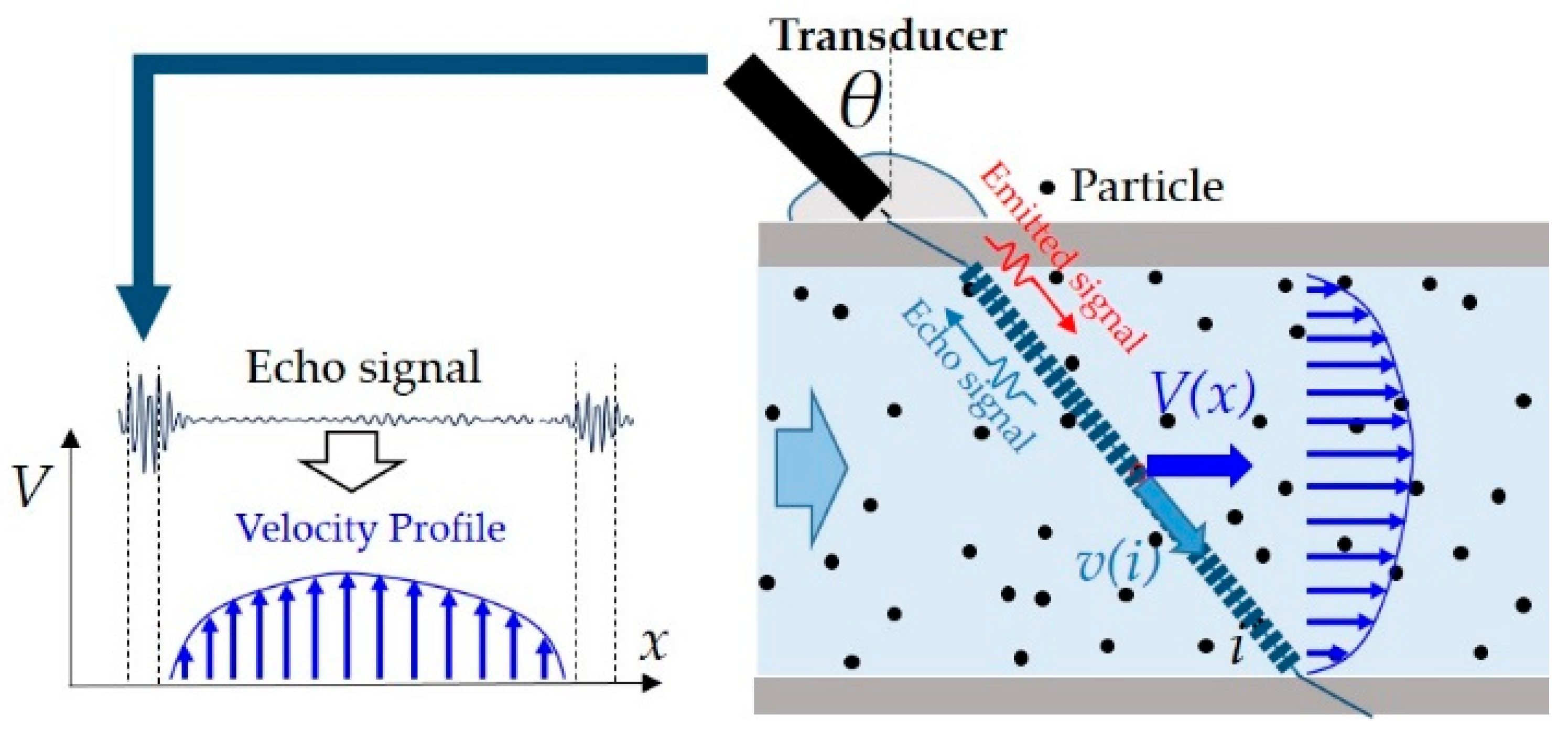
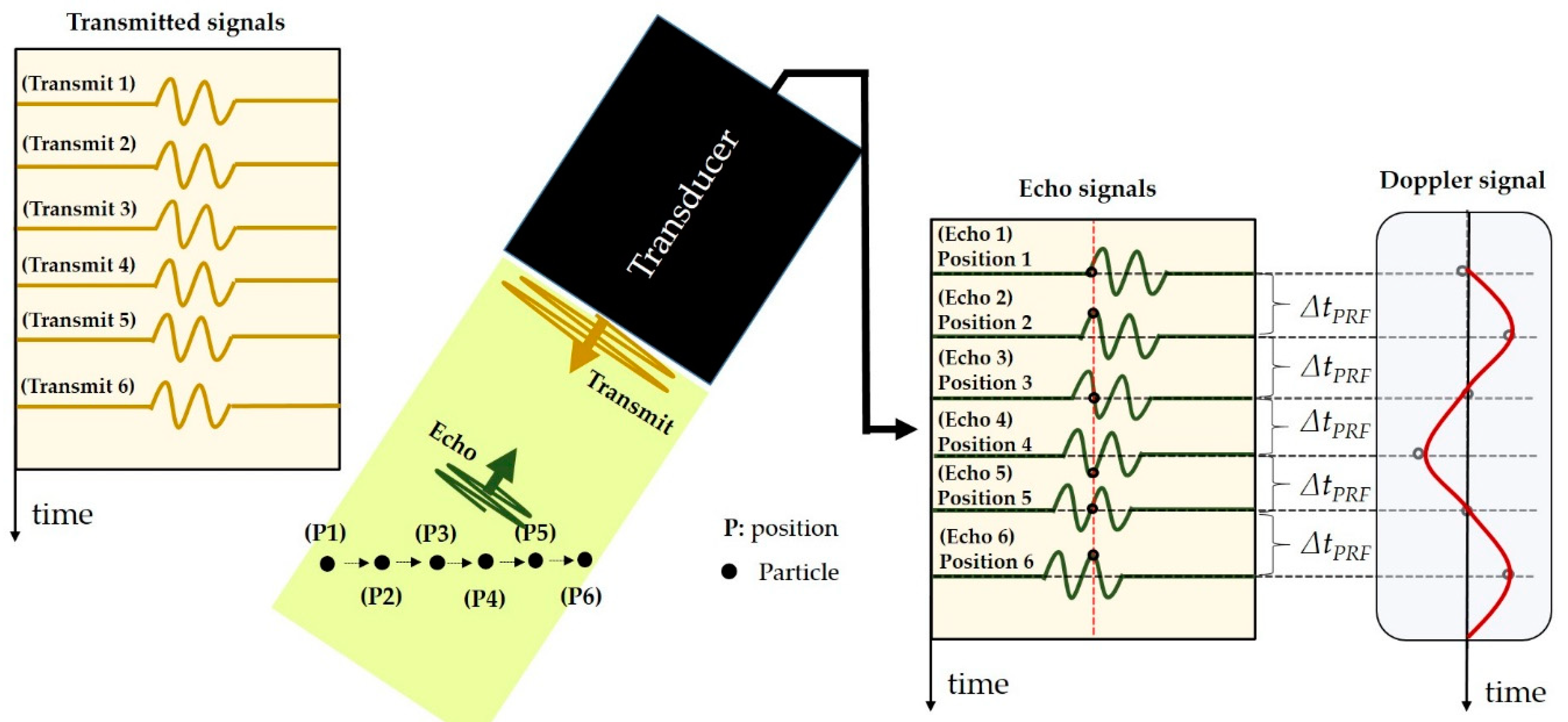
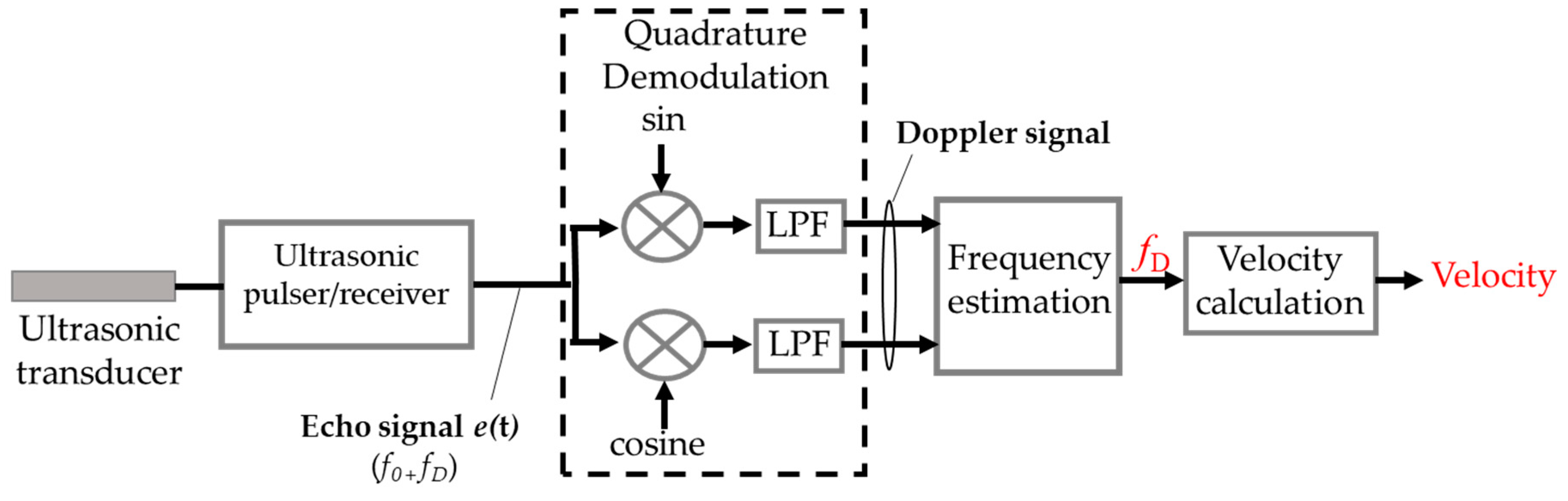
2.1. The UVP with Doppler Pulse Repetition Technique

The UVP method can obtain instantaneous velocity profile of fluid using ultrasonic waves by means of an ultrasound reflector. Figure 1 displays the UVP principle, consisting of ultrasound transmission, an echo signal, and velocity profile obtained. An ultrasonic pulse is emitted repeatedly from the transducer along the measurement line, and the echo reflected from the surface of the reflector such as from a particle is derived from the same transducer. The particles dispersed in the fluid according to the main flow. In the case of water, the density of the particle is nearly equal (0.98 g/cm3). Therefore, the velocity of a particle is assumed to be equal to the velocity of water at that position. The echo signals reflected from moving particles contain the Doppler signal. The Doppler frequency fDi directly relates to the velocity of a moving particle at the position in measuring line. Consequently, the velocity of the particle V(x) can be obtained as follows in Equation (1). The velocity profile of the fluid along the channel diameter can be computed if tracer particles are sufficiently dispersed.
V ( x ) = c f D i 2 f 0 s i n θ
where f0 is the basic frequency of ultrasound, θ is the incident angle, x is a position in the horizontal axis, and i is a position in the measuring line.
The Doppler pulse repetition technique is used to extract the Doppler signal from the echo signal, to estimate the Doppler frequency and calculate fluid velocity, respectively. The Doppler signal can be demodulated from echo signals reflected from a moving particle using ultrasonic emission repetition as shown in Figure 2. Figure 3 shows a block diagram of the UVP system based on the Doppler pulse repetition technique. An ultrasonic pulser/receiver, operated in the pulse-echo mode, emits an ultrasonic pulse through an ultrasonic transducer. The echo signal e(t) is then reflected and sent to the pulser/receiver via the same transducer [23]. It is expressed as:
e ( t ) = A n , i cos 2 π ( f 0 ( t t n , i ) + n f D , i f P R F )
where tn represents the delay time of the echo at nth pulse, A is the amplitude, and fPRF is the pulse repetition frequency.
In the quadrature demodulation section, the echo signals are multiplied by the cosine and sine components, and a finite impulse response filter is then used as a low-pass filter to eliminate the carrier wave component or basic frequency. Therefore, the Doppler signal D(n) can be extracted from the echo signals as modeled in Equation (3)–(6) The Doppler frequency is then estimated in the frequency estimation section by autocorrelation or Fast Fourier Transform [23,24]. Finally, the computed Doppler frequency is plugged into Equation (1) to demonstrate fluid velocity.
Applsci 09 00050 g022 where φ is the initial phase of the in-phase signals XI and the quadrature-phase signals XQ.

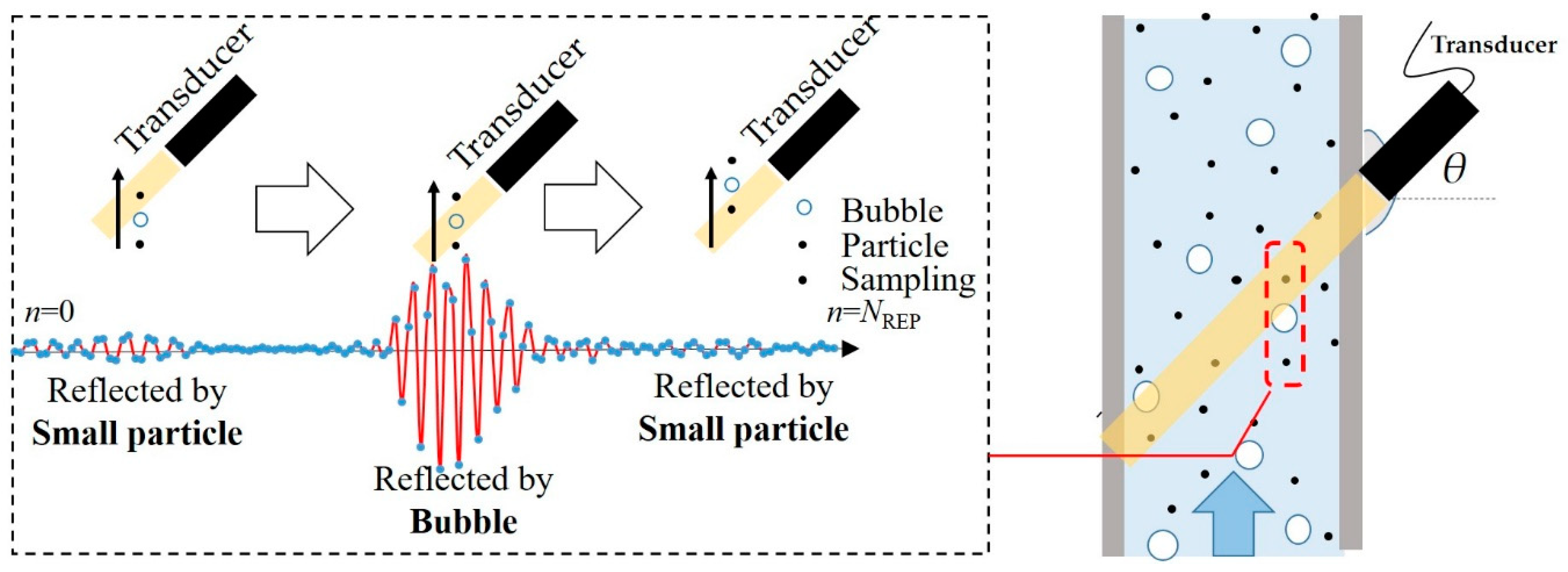
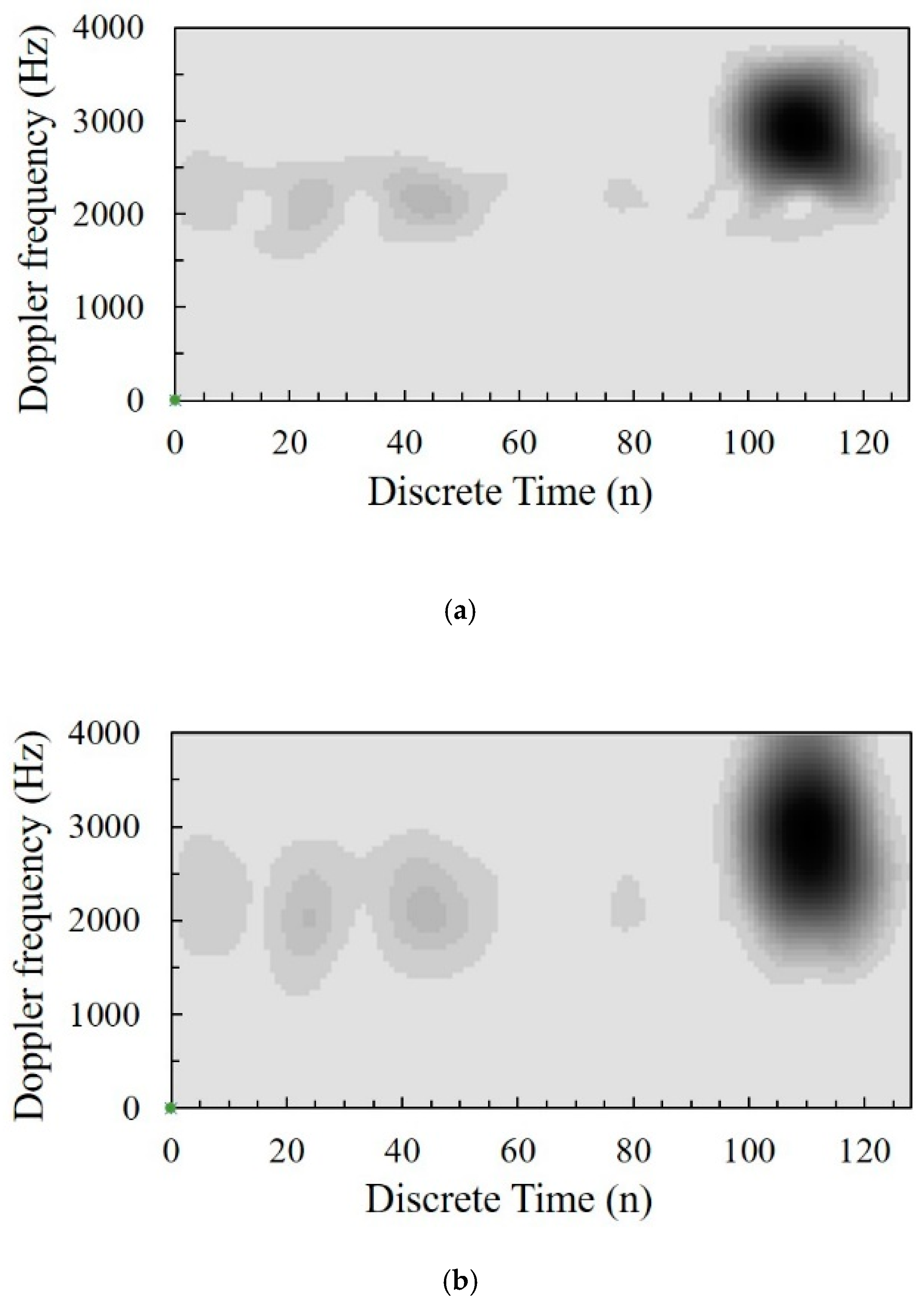
2.2. The Behavior of the Doppler Signal in Two-Phase Bubbly Flow

In two-phase bubbly flow, the Doppler signal is derived from echo signals reflected in a fluid; the echo signals are assessed as either particles or bubbles. Instinctively, the amplitude can indicate its own behavior. Doppler amplitude is considered to be the reflection ratio R of acoustic intensity from the interface point between two media as described by Equation (7):
R = ( Z 1 Z 2 Z 1 + Z 2 ) 2 = ( ρ 1 c 1 ρ 2 c 2 ρ 1 c 1 + ρ 2 c 2 ) 2
where Z represents acoustic impedance, ρ is the density, and c is sound velocity.
The reflection ratio of the gas-liquid interface (bubble) is greater than the solid-liquid interface (particle). Thus, the Doppler amplitude reflected from a bubble is larger than the amplitude from a particle; moreover, Doppler frequencies are still different due to their velocity. In some situations, when the bubble and particle position concurrently occurs at the same measurement channel in accordance with the number of repetitions (NREP), multi-frequency and differences in amplitude can be observed at the Doppler signal as shown in Figure 4. Therefore, to measure and separate the velocity profile of the bubble and particle, the integration of time-frequency analysis and Doppler amplitude classification are proposed in this work to analyze the effect of the Doppler signal.

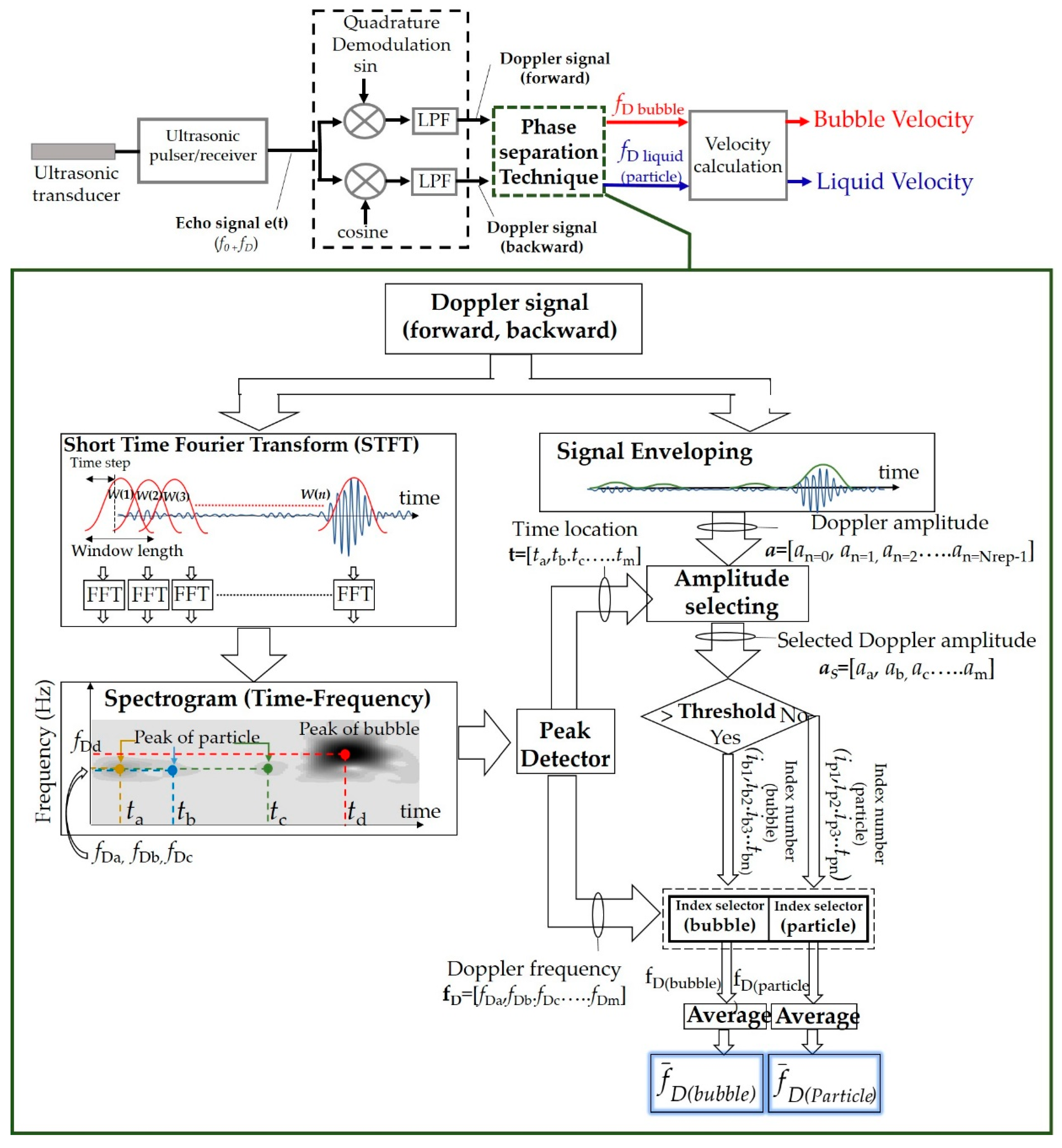
2.3. Phase-Separation Technique

In accordance with the aim of this study, particle and bubble velocities on two-phase bubbly flow can be identified separately by analyzing multi-frequencies and differences in amplitude of the Doppler signal. A technique based on the integration of time-frequency analysis and Doppler amplitude classification is proposed. This technique analyzes both the frequency and amplitude of the signal to decompose Doppler frequency of particle and bubble for obtaining the velocity of both phases separately.
Several types of time-frequency estimator such as STFT, Gabor [25] and Wigner–Ville distribution (WVD) [26] can analyze time-frequency behavior of non-stationary signal which is the same kind of Doppler signal. Each type has advantage and disadvantage. Therefore, the performance of estimators must be evaluated before applying to the measurement system. The performance is evaluated in three indicators; Readability, Resolution and Computational time. The investigation was performed by using one Doppler signal obtained from two-phase bubbly flow as shown in Figure 5. Then, the signal was inputted to the algorithm of three estimators on LabVIEW software. Figure 6a–c are time-frequency spectrogram of Doppler signal obtained from STFT, Gabor and WVD, respectively. The evaluation of three estimators is shown in Table 1 and Table 2. It can be concluded that Short-Time Fourier Transform has a good performance in three criteria (Readability, Resolution and Computational time). Therefore, STFT is selected to be time-frequency estimator in the phase-separation technique.
The STFT analyzes the time-frequency effect of the Doppler signal. The classification of Doppler amplitude is performed by setting a threshold. The threshold value is based on the statistical data of Doppler amplitude reflected by particles and bubbles. The phase-separation technique is applied for operation in the UVP by replacing the frequency estimation section. Figure 7 demonstrates the process of the phase-separation technique.
X ( k , f D ) = n = 0 N R E P 1 D ( n ) W n ( n k S n ) e x p ( j n 2 π f D )
P ( k , f D ) = | X ( k , f D ) | 2
The Doppler signal D(n) is in the form of complex discrete data extracted by the quadrature demodulation section is sent to STFT. The Doppler signal is divided into several windows, and each window is set to overlap with adjacent windows. The signal in each window is then transformed into the frequency spectrum along several short time periods. Its calculation is expressed in Equation (8) and the energy density of spectra at time k is denoted by Equation (9). It is called a time-frequency spectrogram, indicating time-frequency characteristics of the Doppler signal. Its characteristics depend on time step Sn and window length Wn. In this study, for high time resolution, the time step was set equal to 1, and the window length for optimization was a crucial parameter for STFT as it governed the resolutions in both time and frequency. As the window length decreases, the time resolution increases but the frequency resolution in STFT decreases. Therefore, a shorter window length leads to spectral leakage. The methodology used to determine the optimum window length involves a comparison between the frequency analysis of STFT in each window length and the frequency setpoint (simulated signal). In this study, the setpoint value is determined from the Doppler frequency range at fPRF 8 kHz. The maximum Doppler frequency is fDmax = fPRF/2. Therefore, the Doppler frequency range is 0–4 kHz. Figure 8 shows the results of the comparison. The optimum window length is 24. The spectrogram obtained from the STFT is sent to the peak detector. This section analyzes the energy peaks of the spectrogram. Each spectrogram peak value indicates the Doppler frequency data and time location at which the peak occurs. The information is provided in the form of array data—Doppler frequency (fD) and time location (t)—as expressed in Equation (10).
f D = [ f D a , f D b , f D c , f D m ] ,   t = [ t a , t b , t c , t m ]
Furthermore, the amplitude of the Doppler signal at each point is ascertained by making the envelope of the Doppler signal using the Hilbert transform as shown in Equation (11). The data at each point are arranged in array form (a) as Equation (12), and these data are selected by time location index (as) as in Equation (13).
D ( n ) = ( s 2 ( n ) + s ^ 2 ( n ) ) 1 / 2 ,   s ^ ( n ) = d e f H [ s ( n ) ]
a = [ a n = 0 , a n = 1 , a n = 2 , a n = N R E P 1 ]
a S = [ a a , a b , a c , a m ]
The selected data is then compared with a threshold value. The value is defined as being higher than the maximum Doppler amplitude of the particle and lower than the Doppler amplitude obtained from the bubble (the threshold value is determined by the experimental data in Section 4.2). The amplitude data index (i) is separated into two categories as expressed in Equation (14). Firstly, when the amplitude value is higher than the threshold, its index is defined as a bubble index. Secondly, when the value is lower than the threshold, its index is expressed as a particle index. These are called “separation indexes,” and are defined as index selectors. Within these indexes, Doppler frequency data analyzed by peak detector is classified as a Doppler frequency of bubble group and particle group according to Equations (15) and (16). The average Doppler frequency in each group is then shown as Equations (17) and (18). Therefore, the Doppler frequency of bubble and particle in the same measurement channel is classified apparently. Consequently, the velocity of both liquid and bubble can be computed simultaneously.
index ( i ) = def { i bubble   [ i b , i b 1 , , i b ( x 1 ) ] i f   a Si Threshold i particle   [ i p , i p 1 , , i p ( y 1 ) ]   i f   a S i < Threshold
f D ( bubble ) = [ f D b , f D b 1 , , f D b ( x 1 ) ]
f D ( p a r t i c l e ) = [ f D p , f D p 1 , , f D p ( y 1 ) ]
f ¯ D ( b u b b l e ) = f D b + f D b 1 + , , + f D b ( x 1 ) x
f ¯ D ( p a r t i c l e ) = f D p + f D p 1 + , , + f D p ( y 1 ) y
Figure 9a represents an example of the Doppler frequency classification for the proposed technique in one measurement channel, showing the processing system on single-phase flow. The Doppler frequencies observed from the peak on the spectrogram are only influenced by particles because the Doppler amplitude of each time location point is lower than the threshold value. Figure 9b shows the spectrogram in two-phase bubbly flow conditions. The frequency data at points a, and c can be defined as the Doppler frequency of a particle due to Doppler amplitude being lower than the threshold value. On the contrary, at point b, the Doppler frequency belongs to a bubble because Doppler amplitude is higher than the threshold value.

3. Experimental Setup

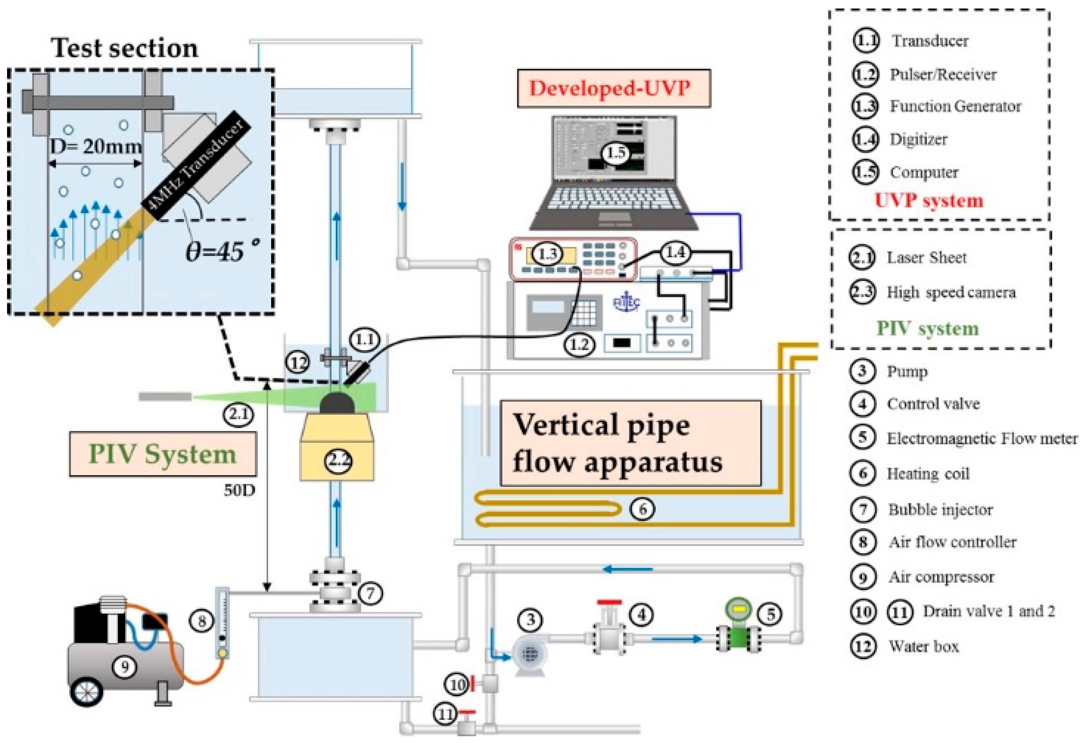
3.1. Experimental Apparatus

Figure 10 shows a schematic diagram of the experimental apparatus. The UVP measurement with a phase-separation technique called Developed-UVP consists of a 4 MHz ultrasonic transducer, an ultrasonic pulser/receiver, a function generator, a digitizer, and a computer with LabVIEW software as shown in Table 3. The pulser/receiver emitted (the pulse shape was programmed by function generator) and received ultrasonic pulses through an ultrasonic transducer. The echo signals received by the pulser/receiver were converted to a digital signal by the digitizer, with a sampling rate of 100 MS/s. The digitizer and pulser/receiver were connected and synchronized with each other. Data from the digitizer were recorded on the computer via USB port. Calculation and analysis were performed using LabVIEW software. The measurement test section was located on a vertical pipe made up of acrylic with an inner diameter (D) of 20 mm. The measurements were conducted downstream at a distance of 50 D from a bubble injector. The transducer was positioned on a clamper at the outer surface of the pipe with an incident angle of (θ) 45°. This incident angle, the ultrasound transmission ratio is maximum. Also, two wave mode (Longitudinal and Shear wave) does not occur. Therefore, incident angle 45 degree was chosen in this study. [27]. The working fluid was water. Its temperature was measured by a thermocouple and controlled to produce a small deviation at 25 ± 2 °C by a cooling system. The most important liquid phase properties on two-phase flow regime is liquid viscosity. Weiman et al. [28] investigated the influence of liquid viscosity and pipe diameter on the flow regime. They concluded that liquid viscosity and pipe diameter did not significantly affect the transitions between flow regimes. However, in the UVP measurement, liquid temperature is very important properties. The speed of sound is a function of temperature; therefore, the liquid temperature should be monitored during the experiment. Then, nylon particles of 80 µm were dispersed into the water as tracer of the liquid. The air was injected from a bubble injector to generate the bubble using an air compressor. In this work, the basic frequency of ultrasonic wave was 4 MHz which is in high frequency range. High frequency will reduce cavitation effect because the negative pressure produced by rarefaction cycle is insufficient in duration and intensity to initiate cavitation. The sound pressure in the liquid at this frequency is very small. Hence, the bubbles (cavitation) are not produced [29]. As a consequence, condensation and evaporation process could not occur in this experiment.

3.2. Experimental Conditions and Procedure

Firstly, the experiment was conducted to measure the velocity profiles on single-phase liquid (water) flow at a superficial liquid velocity UL of 200 mm/s and 300 mm/s, respectively (Reynolds numbers: 3699 and 5549). The Developed-UVP performance was compared using the PIV and the Original-UVP (autocorrelation) methods. A summary of the experimental conditions is shown in Table 4. The Developed-UVP, Original-UVP and PIV parameters were set for compatibility with experimental conditions as shown in Table 5 and Table 6.
Secondly, for separating the velocity of the bubble and liquid phases in bubbly flow, the Doppler amplitude threshold must be set. To set the threshold value, Doppler amplitude testing was carried out on two reflector conditions dispersed in fluid flow: (1) nylon particles 80 µm (liquid phase); and (2) a large number of microbubbles at diameter <1 mm (bubble phase). The testing was conducted at a UL of 200 mm/s and 300 mm/s, respectively. The evaluation was then obtained by observing the amplitude value of 30,000 Doppler signals in each condition.
Thirdly, an experiment was conducted to measure the velocity profile of the two-phase bubbly flow. In this study, the bubbles coalescence and break-up should not be occurred in the measurement volume; therefore, to avoid a complex bubbles behavior on measurement volume, the experiment was conducted in the homogeneous flow regime. The homogeneous flow regime (associated with small superficial gas velocities, UG) is referred as the flow regime where only “non-coalescence- induced” bubbles exist [30]. The “homogeneous flow regime”, can be classified into mono-dispersed homogeneous flow regime and pseudo-homogeneous flow regime depending on the prevailing bubble size distributions. Coalescence and break-up kernels can be neglected in certain cases (i.e., mono-dispersed homogeneous flow regime and the pseudo-homogeneous flow regime, when C&B are restricted to small areas in the domain) [31]. In this experiment, the UL was set at 200 mm/s and 300 mm/s. The superficial gas velocity UG injected by the bubble injector was 5.3 mm/s. It was confirmed by visual observations (high speed camera) that neither bubbles coalescence nor break-up was not observed during the experiment. The bubble diameter was about 2–3 mm. Furthermore, the nylon particles dispersed in the water were tracers for the liquid phase. The bubble and liquid velocity profiles after separation by means of Developed-UVP were validated using the PIV.
Lastly, the effect of the void fraction was clarified. An experiment was conducted to measure the velocity profile of the two-phase bubbly flow at different void fractions with constant bubble size at UL 200 mm/s.

4. Results and Discussion

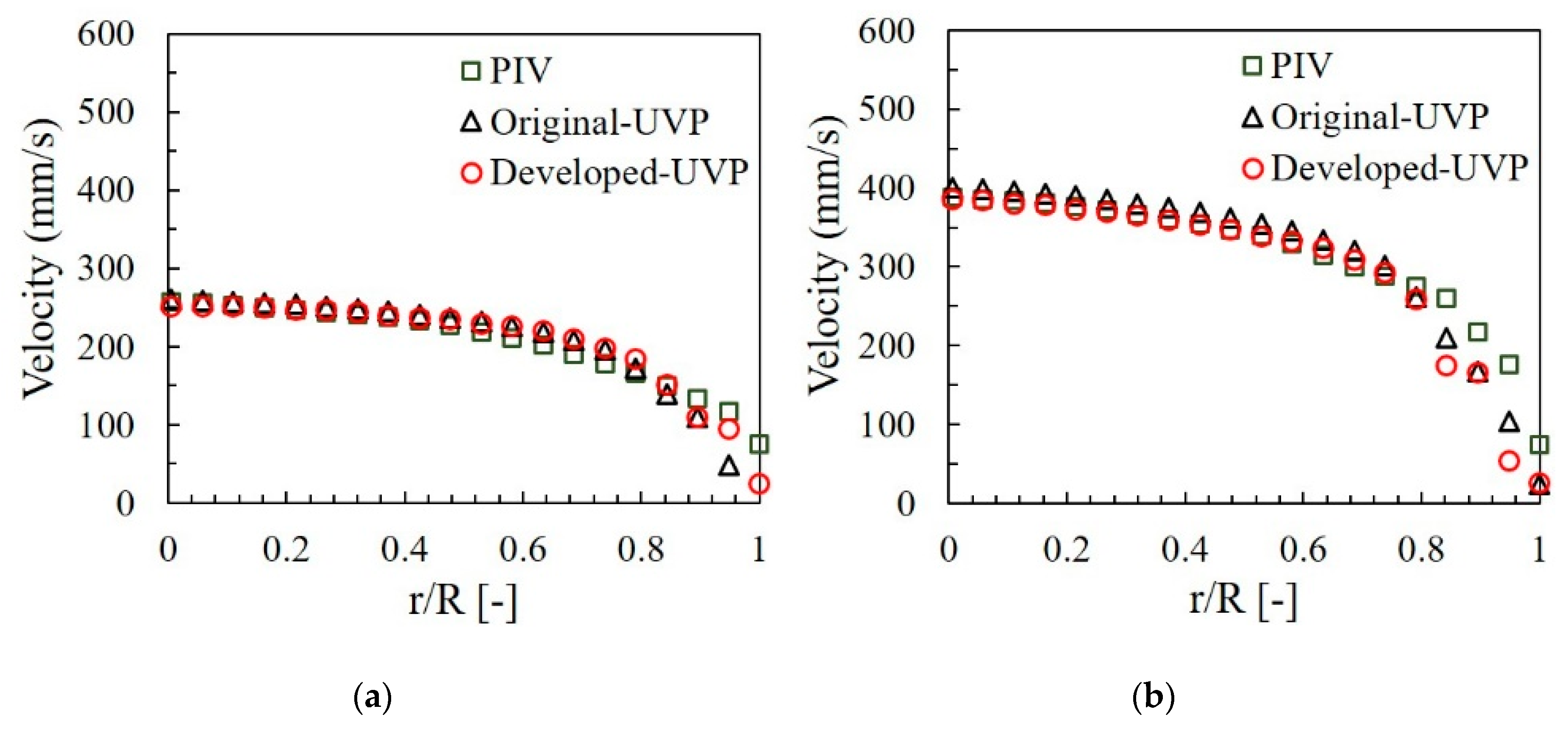
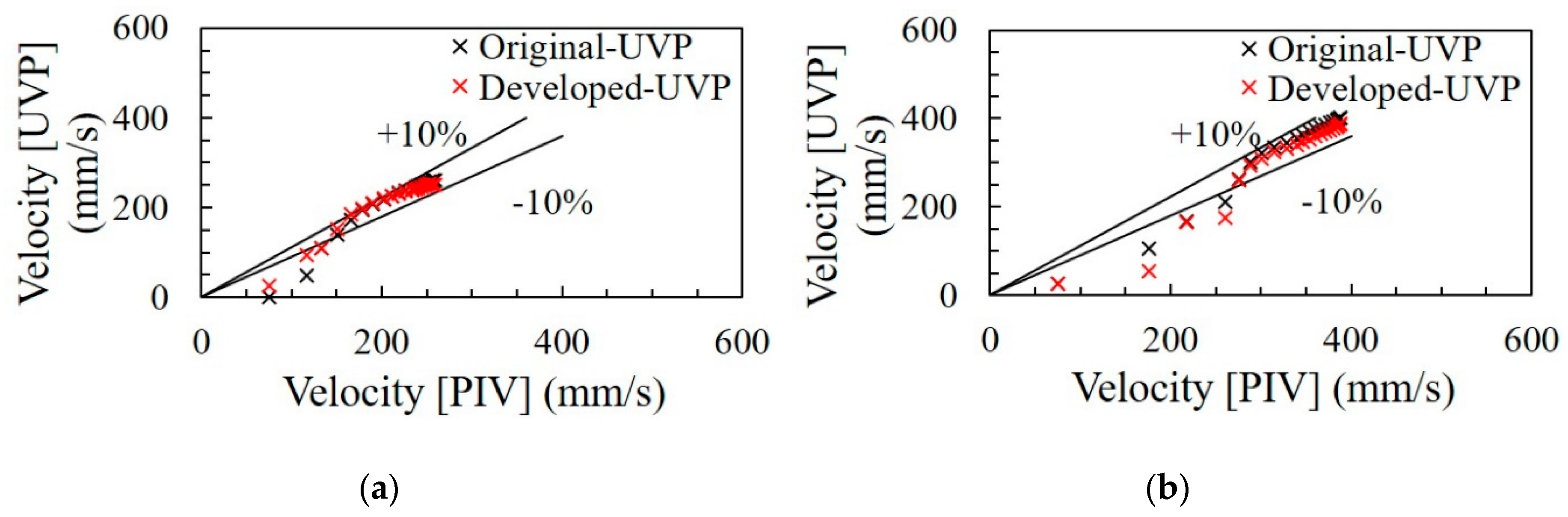
4.1. Velocity Profile Measurement at Single-Phase Flow

Figure 11a,b show the results of averaging data of 5000 instantaneous velocity profile in single-phase liquid flow at the UL of 200 and 300 mm/s. The horizontal axis indicates the distance from the wall (r) nominalized by the pipe radius (R). The measurement results of Developed-UVP were calibrated with PIV and Original-UVP. The velocity distributions measured by Developed-UVP, PIV, and Original-UVP, were almost in agreement. However, the velocity distribution of UVP near the vicinity of the wall showed small fluctuations due to some parts of the ultrasonic measurement volume is located within the wall which is the overlapped regions between the ultrasonic wave and pipe wall [32,33]. The echo data is not only affected by the particle. Hence, the measurement result at that zone is influenced by moving particles and the pipe wall. Figure 12a,b illustrate the accuracy evaluation represented by the discrepancy of results between Developed-UVP, Original-UVP, and PIV methods. The deviation between these methods was within the acceptable range of ±10% at a radius ratio of <0.8. However, a few points at the near-wall zone were out of the acceptable range. Therefore, it can be concluded that Developed-UVP efficiently measured the velocity profile on a single-phase flow since it appeared to be in good agreement with the measurement results obtained using PIV and Original-UVP methods.

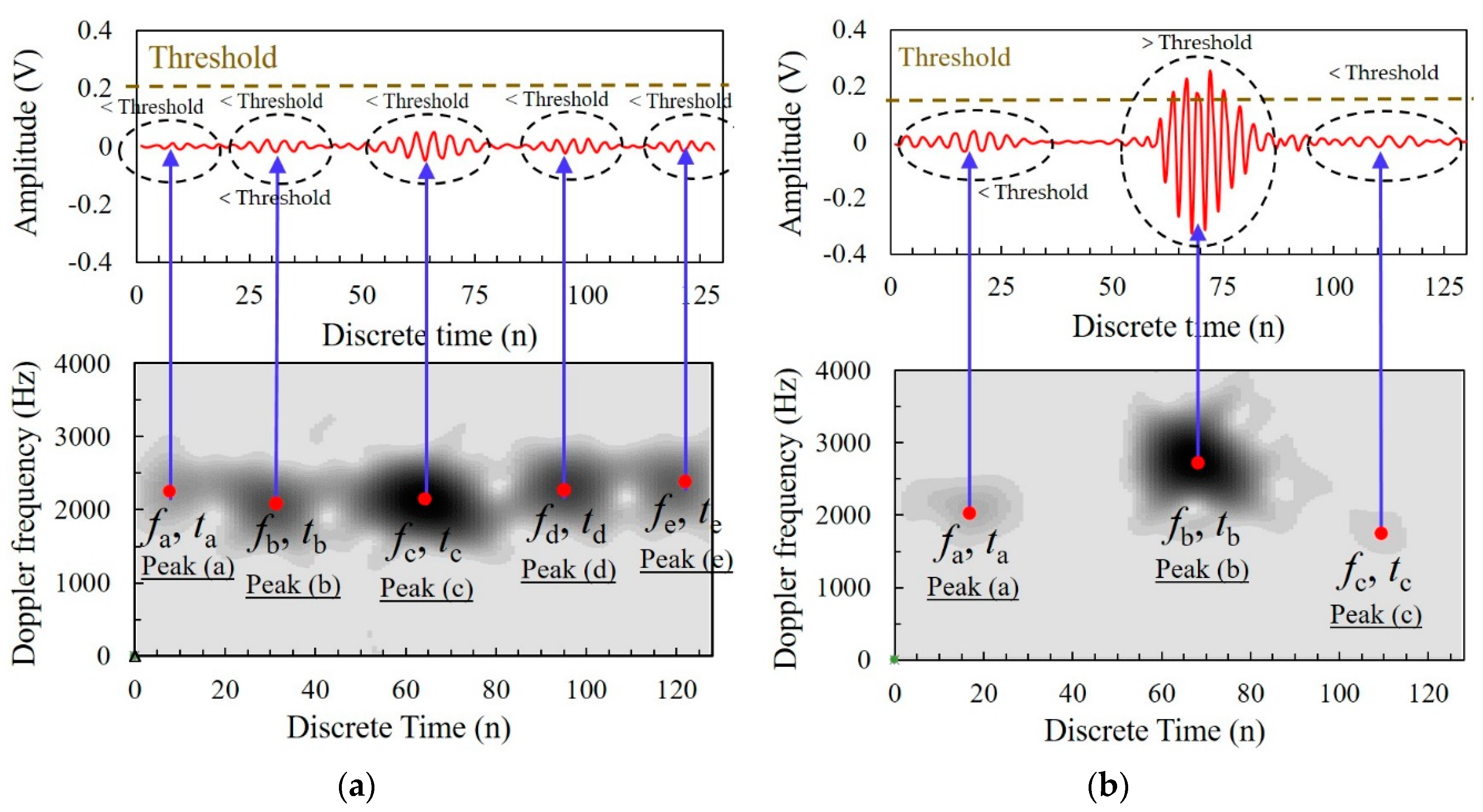
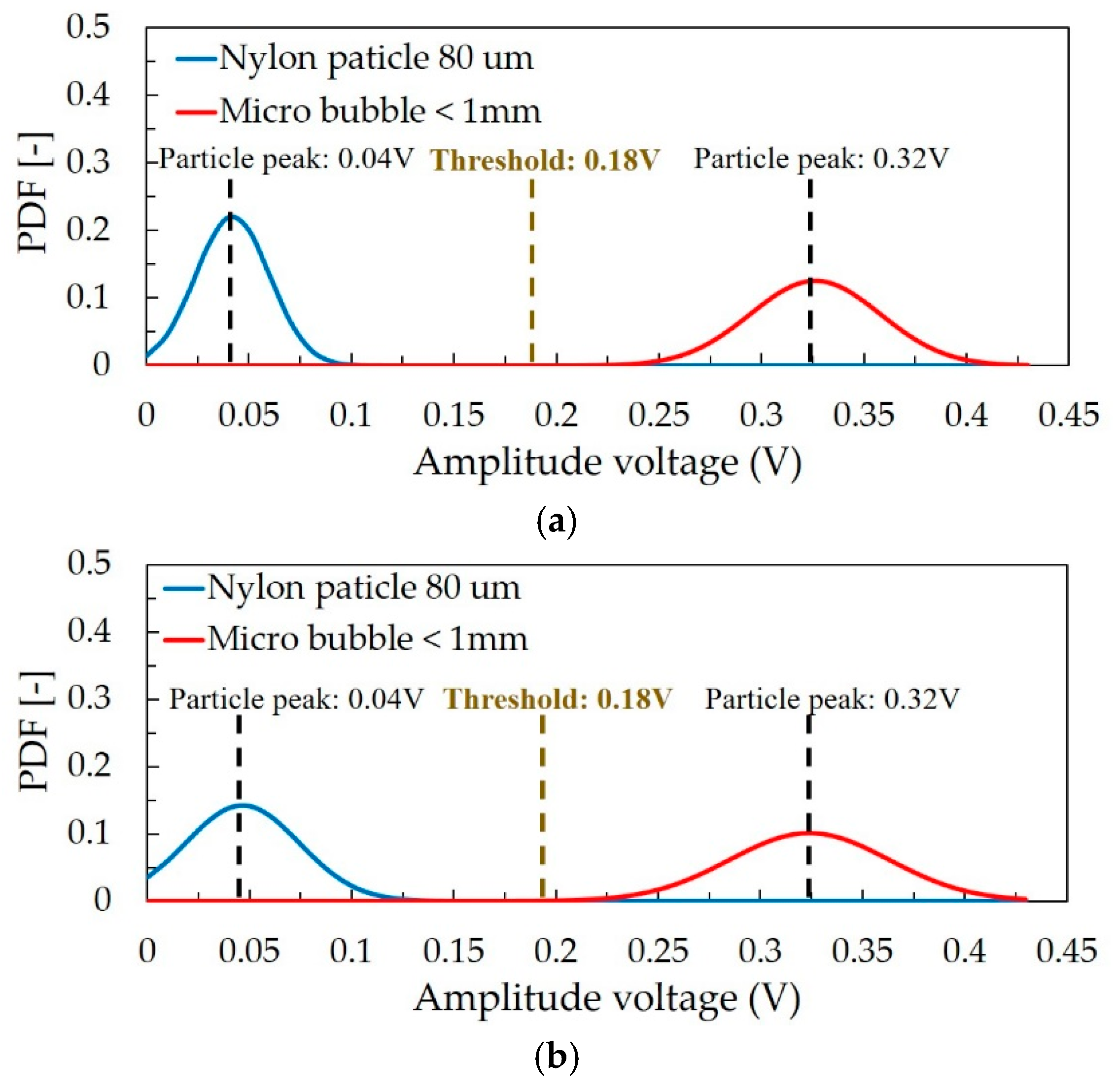
4.2. Doppler Amplitude Threshold Setting

Figure 13 represents the probability density function (PDF) of Doppler amplitude reflected in two conditions; nylon particles 80 µm and microbubbles <1 mm at UL: 200 mm/s and 300 mm/s, respectively. An evaluation was carried out by observing the maximum of Doppler amplitude data of 30,000 Doppler signals in each condition. Whenever a nylon particle was dispersed into the water, the distribution of PDF of Doppler amplitude voltage occurred during 0–0.1 V at UL: 200 mm/s and 300 mm/s. The peak was observed at about 0.04 V. Furthermore, a large number of bubbles at the microscale (diameter <1 mm) were injected into the water without any nylon particles. Clearly, the PDF of Doppler amplitude voltage was distributed between 0.25 V and 0.4 V at both velocity levels of liquid. The peak was observed at about 0.32 V. Hence, it can be concluded that the Doppler amplitude reflected by a particle and bubble is obviously different.
The setting of the threshold value, to precisely separate Doppler amplitude reflected by both reflectors, was done on PDF of Doppler amplitude. Therefore, the threshold was set at about 0.18 V which was the center point between the peak of PDF of particle and bubble. At both velocity levels; UL: 200 mm/s and 300 mm/s, the probability (β) of occurring of bubble data in particle zone (lower than the threshold value) was less than 0.01. Also, the value of particle data that occur within the region of bubble data (Higher than the threshold value) was smaller than 0.01.

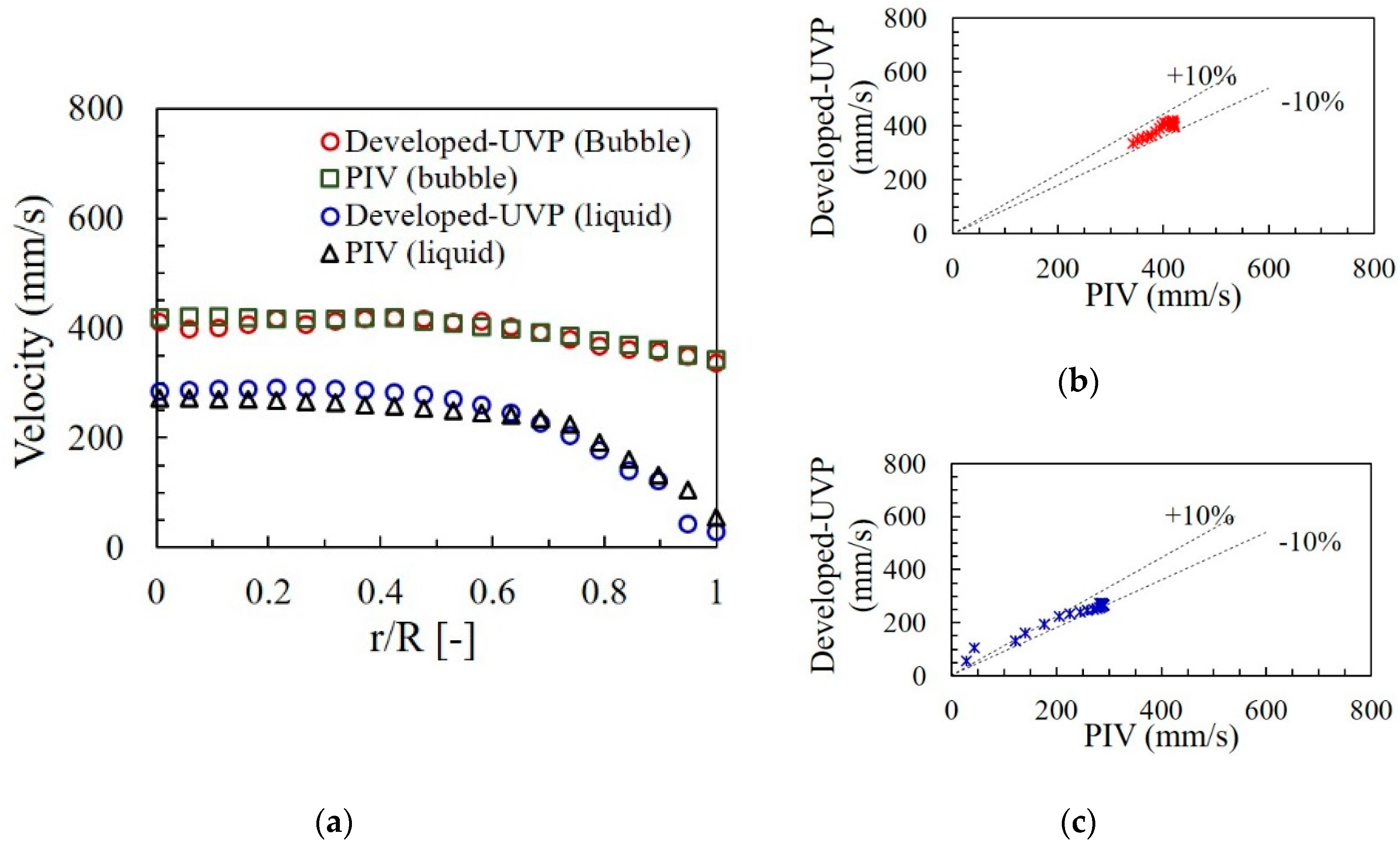
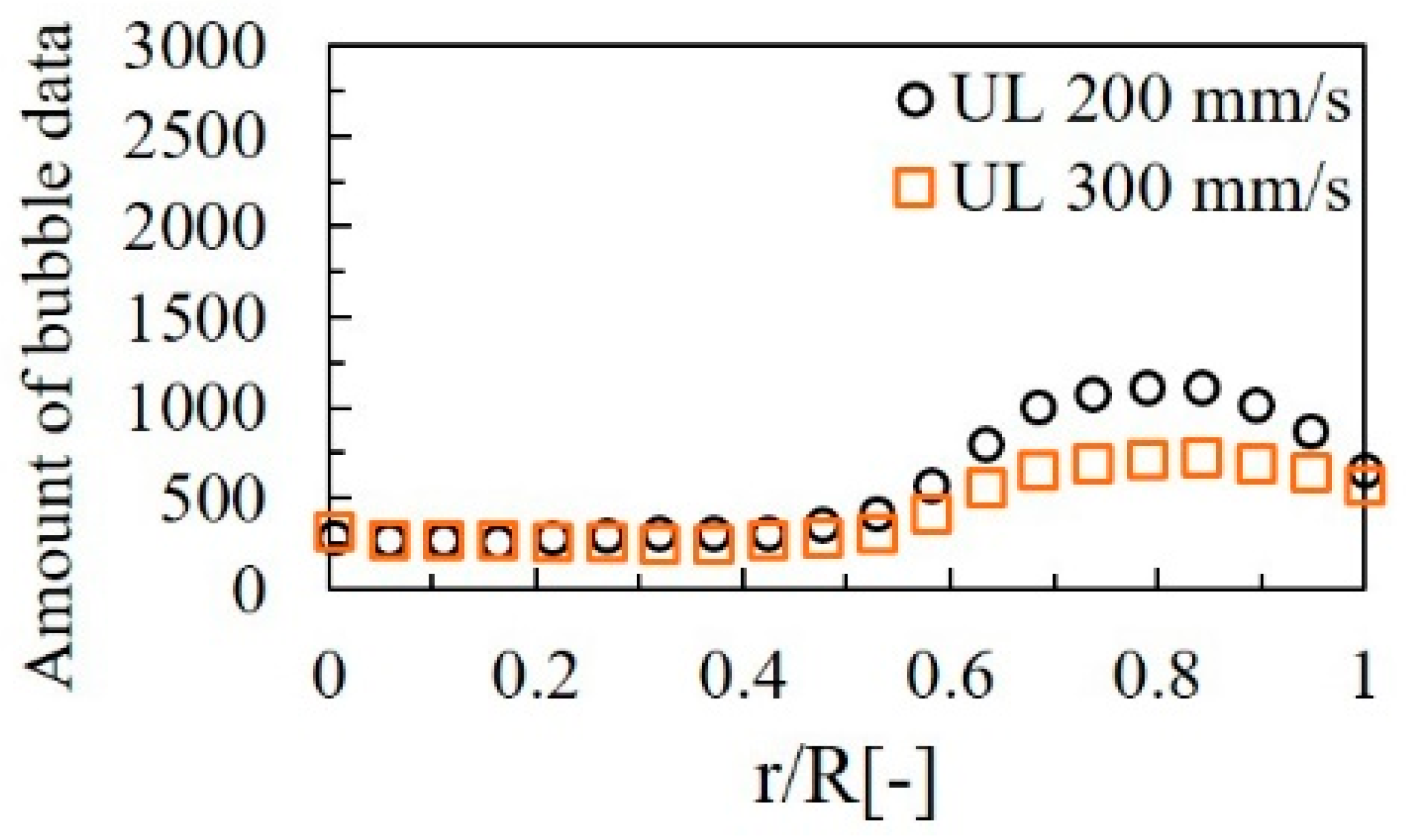
4.3. Velocity Profile Measurement at Two-phase Bubbly Flow

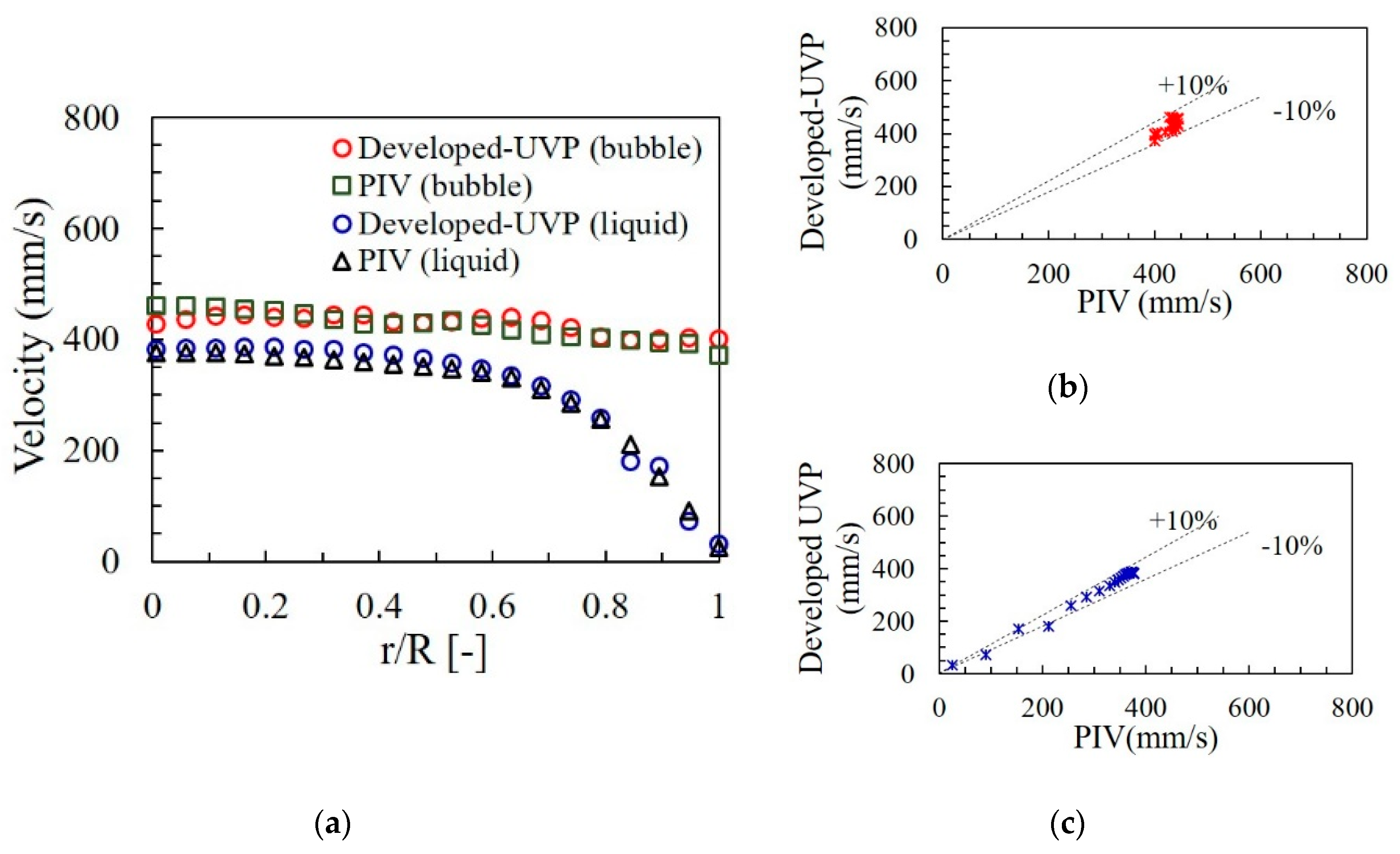
4.3.1. Measurement and Comparison

The experiment was conducted at UL = 200 mm/s and UG = 5.3 mm/s as shown in Figure 14. The bubble diameter in this experiment was about 2–3 mm. Figure 15a shows the measurement results of two-phase bubbly flows. Bubbles rise mainly near the wall region. The graph shows the average velocity profile data. Liquid velocity distribution is the mean of 5000 profiles and bubble rising velocity is averaged by the amount of data obtained as shown in Figure 16. The result of bubble velocity distribution after separation by the Developed-UVP technique was verified using the PIV method. The velocity profiles of bubble measured by both methods were almost coincident with each other. It was confirmed that discrepancy of both systems was within an acceptable range of ±10% as shown in Figure 15b. Furthermore, the liquid velocity profile was obtained and separated from the bubble phase obviously. The result was compared with the liquid phase result of the PIV. The discrepancy between these methods was within the acceptable range of ±10% except a few points at the near-wall zone as illustrated in Figure 15c. However, the liquid velocity profile measurement of Developed-UVP in two-phase bubbly flow can be confidently trusted owing to deletion of the bubble velocity data and had good agreement with PIV method.
Next, The UL increased to 300 mm/s, but gas superficial velocity remained similar to the previous case. The bubble diameter was still about 2–3 mm. Figure 17a represents that the velocity profile of bubble and liquid was obtained separately. Good agreement in the velocity profile measurement of both phases was observed between the Developed-UVP and PIV method due to the discrepancy of both systems was within an acceptable range of ±10% as illustrated in Figure 17b,c, respectively.
From the results at both velocity levels, the measurement error of the bubble and liquid velocity could be caused by measuring equipment, methodology and the experimental condition. Also, the amount of bubble data and void fraction affect the averaging result of bubble velocity. Furthermore, the velocity distribution of bubble and liquid separated had an error at near the wall region (near-wall effect). The error analysis is explained in the detail in Section 4.4.

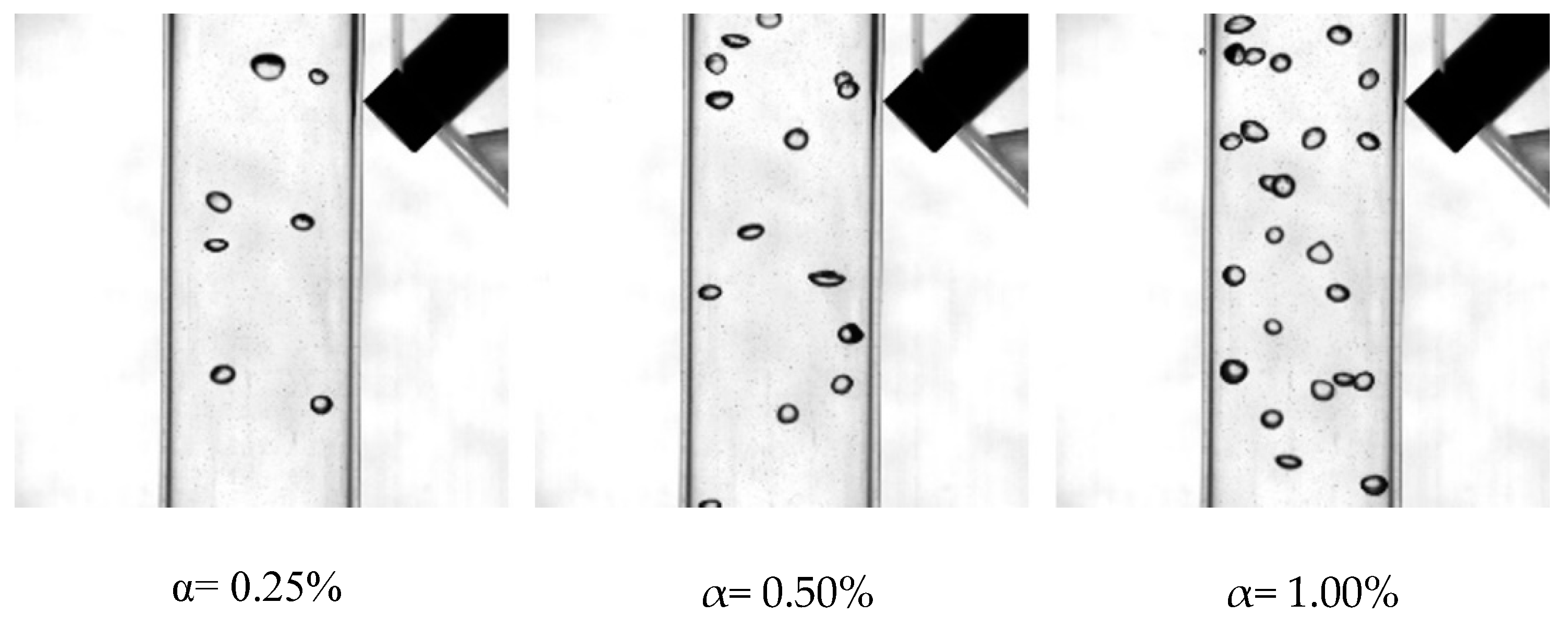
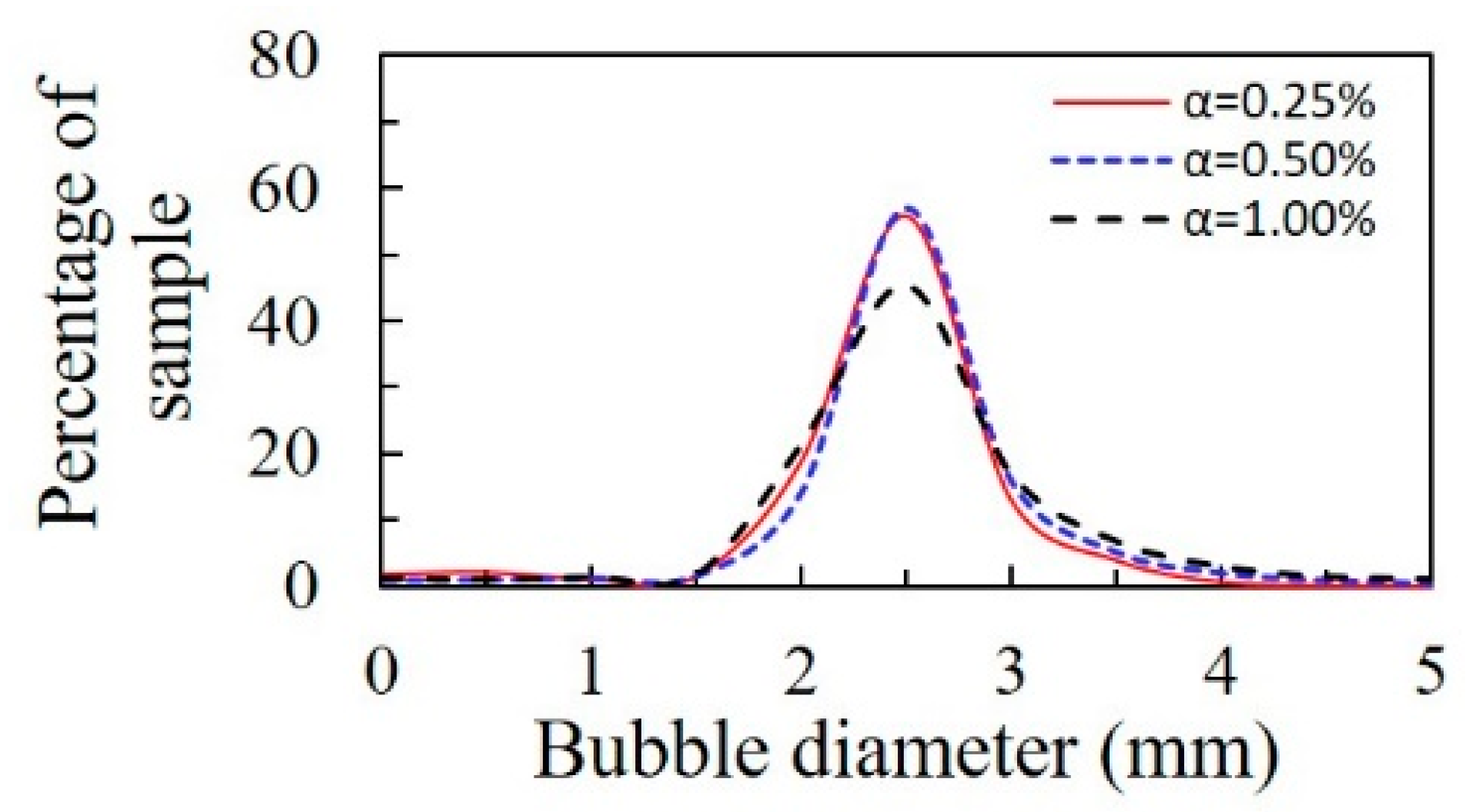
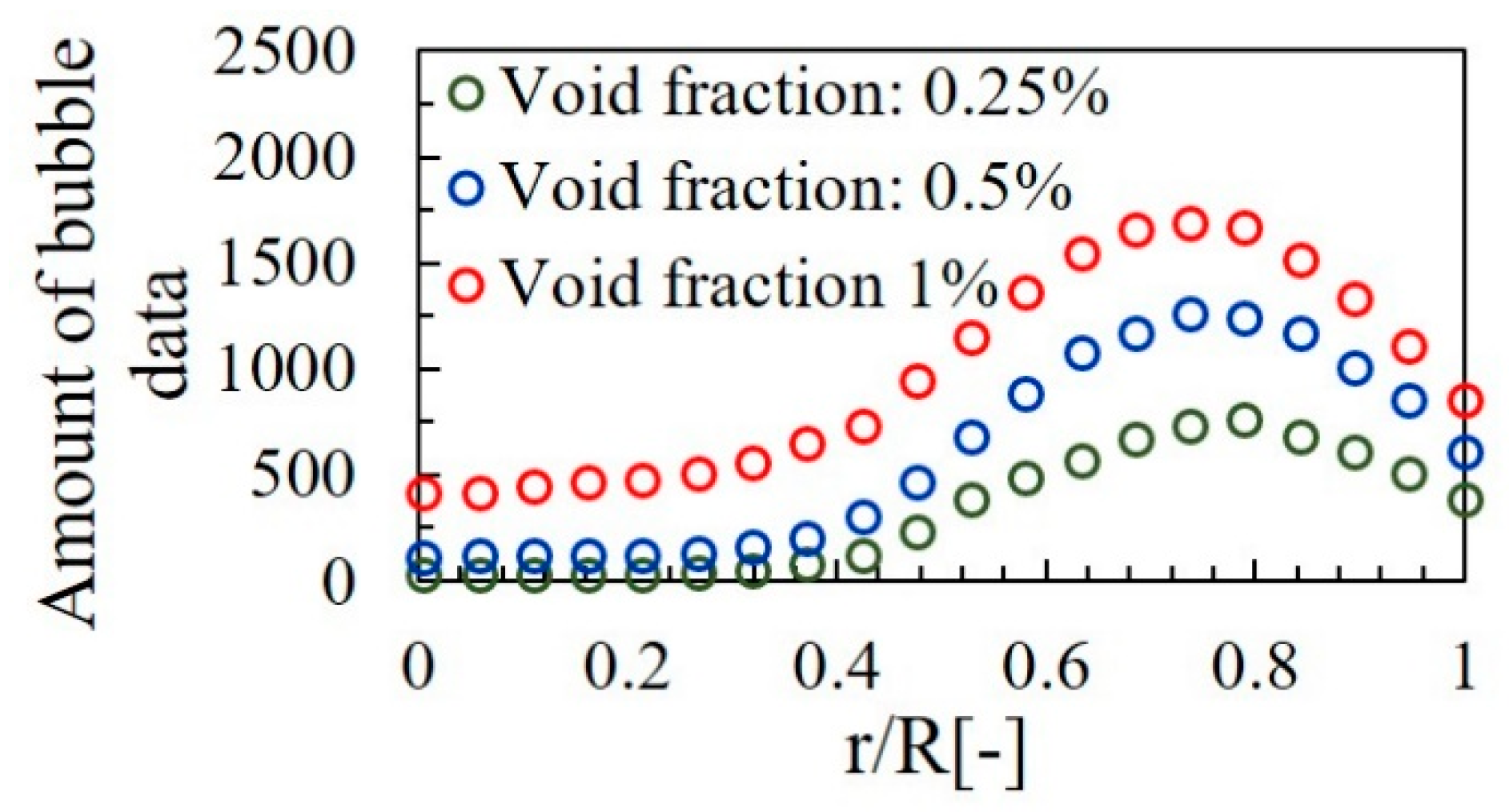
4.3.2. Measurement at a Different Void Fraction

The experiment was conducted on UL = 200 mm/s at different void fraction (α); 0.25%, 0.50% and 1.00%. From the visual observations as shown in Figure 18, the bubble shape was mostly spherical. In the present study, the effects of different bubble shapes will not be taken into account. It was confirmed that the flow regime was mono-dispersed flow regime with the bubble diameter was about 2–3 mm as represented in Figure 19. In this flow regime, the bubbles are uniformly distributed in the cross-section of the pipe, traveling vertically with minor transverse and axial oscillations [34]. Figure 20 represents the measurement results obtained by Developed-UVP. The graph shows the average velocity profile of both phases. The liquid velocity profile is the mean of 5000 profiles and bubble velocity profile is averaged by the amount of data obtained as shown in Figure 21.
The result of bubble velocity in each void fraction was almost coincident with each other except the data of α: 0.25% at center pipe region. The fluctuation within this zone was caused by a small number of averaging data. Furthermore, the liquid velocity profiles could be obtained separately. The profile of liquid rises obviously when void fraction increases due to the enhancement of several bubbles. Hence, It can be concluded that the void fraction with constant bubble diameter affects the velocity level of the liquid. Besides, it influences measurement error of bubble velocity, if the void fraction is very low.

4.4. Error Analysis

The measurement error of the Developed-UVP was analyzed. Basically, it is a combination of systematic error and random error. Various sources of systematic error are investigated and listed in Table 7. These errors are mainly influenced by equipment and methodology. Firstly, a basic frequency at 4MHz that was emitted by the pulser/receiver. Secondly, the sound velocity which was affected by temperature variation. Thirdly, the incident angle of transducer installation. Lastly, Doppler frequency which was mainly affected by pulse repetition frequency, time lapse and frequency estimation of the developed algorithm. However, the error of pulse repetition frequency and time-lapse could be ignored due to the error magnitude was very small when compared with the error of frequency estimation. Consequently, the error of Doppler frequency was mostly involved by the frequency estimation of the developed algorithm. Therefore, the systematic error can be obtained by combining each error component as represented in equation 16 which is 3.02%. The main factor of systematic error is the incident angle.
%   error   of   V i = ( Δ V i V i ) × 100 = ( Δ c c ) 2 + ( Δ f D i f D i ) 2 + ( Δ f 0 f 0 ) 2 + ( Δ sin θ sin θ ) 2 × 100
where ∆ is error magnitude of each parameter.
The random error also affects the measurement accuracy. This error was unpredictable due to fluctuation or instability of the experimental condition occurred randomly that influenced by some phenomena such as the multi-dimensional motion of bubble and particle, and noises which exclude the influences of measuring equipment and methodology. Therefore, if these errors do not occur, the measurement error can be most affected by the systematic error.
Considerably, within the near wall region (at a radius ratio between 0.8 and 1.0), the error occurred which caused by the near-wall effect. This is an effect of the wave overlapping between the wall region and the measuring fluid. The effect cannot be avoided. It is included in systematic error. However, the error from other sources can be ignored owing to the error magnitude was significantly lower than the error obtained from this effect. Therefore, within this zone, the measurement error is mainly influenced by near-wall effect.

5. Conclusions

A UVP method for measuring the instantaneous velocity profiles of liquid and bubbles in two-phase bubbly flow has been developed. Instantaneous velocity profiles of single-phase and two-phase bubbly flow have been measured experimentally. The developed system employs only a single resonant frequency. Therefore, extra equipment is not needed. Signal processing, based on the Doppler pulse repetition technique, has been modified by applying the integration of Short-Time Fourier Transform and Doppler Amplitude Classification. The Developed-UVP can decompose the Doppler frequency of a particle (liquid phase) and bubble. Hence, the velocity distribution of the liquid and bubble can be measured and separated clearly. The experiment was conducted on vertical pipe flow apparatus, and measurement comparison was performed using PIV method. The measurement results clarify that the Developed-UVP is in good agreement with the PIV. Moreover, the effect of void fraction against velocity measurement of both phases was demonstrated. Therefore, it can be concluded that the Developed-UVP can measure liquid and bubble velocity simultaneously in the two-phase bubbly flow.
The Developed-UVP has the following main advantages.
-
Instantaneous velocity profile of liquid and bubble can be obtained simultaneously.
-
The velocity profile of liquid and bubble can be separately obtained even if the velocity data of both phases occur in the same measurement channel.
-
The developed phase separation can distinguish the velocity of both phases, although similarities occur with both phases.
-
The system requires only a single resonant frequency transducer, a single channel pulser/receiver, and basic data processing equipment.
Nevertheless, the developed technique is promising. Consequently, the technique can be applied to scale-up to industrial units. The further study on the applying of developed technique to industrial scale will be our future study.

Author Contributions

The work presented in this paper was a collaboration of all authors. W.W., A.H., N.T.-u, H.T. and H.K. Methodology; W.W., A.H. and N.T.-u, Project administration; H.T. and H.K., Supervision; H.K. Analyzing the data; W.W., A.H. and N.T.-u, Writing the paper; W.W., which was discussed and revised by all authors.

Acknowledgments

The authors are grateful for the support of Ministry of Education, Culture, Sports, Science and Technology (MEXT).

Conflicts of Interest

The authors declare no conflicts of interest.

References

  1. Ishii, M.; Hibiki, T. Thermo-Fluid Dynamics of Two-Phase Flow; Springer: New York, NY, USA, 2012. [Google Scholar]
  2. Ozaki, T.; Suzuki, R.; Mashiko, H.; Hibiki, T. Development of drift-flux model based on 8 × 8 BWR rod bundle geometry experiments under prototypic temperature and pressure conditions. J. Nucl. Sci. Technol. 2013, 50, 563–580. [Google Scholar] [CrossRef] [Green Version]
  3. Wang, G.; Ching, C.Y. Measurement of multiple gas-bubble velocities in gas-liquid flows using hot-film anemometry. Exp. Fluids 2001, 31, 428–439. [Google Scholar] [CrossRef]
  4. Wu, Q.; Ishii, M. Sensitivity study on double-sensor conductivity probe for the measurement of interfacial area concentration in bubbly flow. Int. J. Multiph. Flow 1999, 25, 155–173. [Google Scholar] [CrossRef]
  5. Muñoz-Cobo, J.L.; Chiva, S. Development of Conductivity Sensors for Multi-Phase Flow Local Measurements at the Polytechnic University of Valencia (UPV) and University Jaume I of Castellon (UJI). Sensors 2017, 17, 1077. [Google Scholar] [CrossRef] [PubMed]
  6. Albrecht, H.E.; Borys, M.; Damaschke, N.; Tropea, C. Laser Doppler and Phase Doppler Measurements Techniques; Springer: Berlin/Heidelberg, Germany, 2003. [Google Scholar]
  7. Chen, R.C.; Fan, L.S. Particle image velocimetry for characterizing the flow structure in three- dimensional gas-liquid-solid fluidized beds. Chem. Eng. Sci. 1992, 47, 3615–3622. [Google Scholar] [CrossRef]
  8. Lindken, R.; Merzkirch, W. Velocity measurements of liquid and gaseous phase for a system of bubbles rising in water. Exp. Fluids 2000, 29, 194–201. [Google Scholar] [CrossRef]
  9. Takeda, Y. Velocity profile measurement by ultrasonic Doppler shift method. Int. J. Heat Fluid Flow 2008, 7, 313–318. [Google Scholar] [CrossRef]
  10. Aritomi, M.; Zhou, S.; Nakajima, M.; Takeda, Y.; Mori, M.; Yoshioka, Y. Measurement system of bubbly flow using ultrasonic velocity profile monitor and video data processing unit. J. Nucl. Sci. Technol. 1996, 33, 915–923. [Google Scholar] [CrossRef]
  11. Aritomi, M.; Zhou, S.; Nakajima, M.; Takeda, Y.; Mori, M.; Yoshioka, Y. Measurement system of bubbly flow using ultrasonic velocity profile monitor and video data processing unit (II) Flow characteristic of bubbly counter current flow. J. Nucl. Sci. Technol. 1997, 34, 783–791. [Google Scholar] [CrossRef]
  12. Zhou, S.; Suzuki, Y.; Aritomi, M.; Matsuzaki, M.; Takeda, Y.; Mori, M. Measurement system of bubbly flow using ultrasonic velocity profile monitor and video data processing unit (III) Comparison of flow characteristics between bubbly current and counter current flow. J. Nucl. Sci. Technol. 1998, 35, 335–343. [Google Scholar] [CrossRef]
  13. Suzuki, Y.; Nakagawa, M.; Aritomi, M.; Murakawa, H.; Kikura, H.; Mori, M. Microstructure of the flow field around a bubble in counter-current bubbly flow. Exp. Therm. Fluid Sci. 2002, 26, 221–227. [Google Scholar] [CrossRef]
  14. Yamanaka, G.; Murakawa, H.; Kikura, H.; Aritomi, M. The novel velocity profile measuring method in bubbly flows using ultrasound pulses. In Proceedings of the 7th International Symposium on Fluid Control, Measurement and Visualization, Sorento, Italy, 25–28 August 2003; pp. 214–217. [Google Scholar]
  15. Murakawa, H.; Kikura, H.; Aritomi, M. Application of ultrasonic multi-wave method for two-phase bubbly and slug flow. Flow Meas. Instrum. 2008, 19, 205–213. [Google Scholar] [CrossRef]
  16. Nguyen, T.; Murakawa, H.; Tsuzuki, N.; Kikura, H. Development of multi-wave method using ultrasonic pulse. J. Jpn. Soc. Exp. Mech. 2013, 13, 277–284. [Google Scholar]
  17. Murai, Y.; Tasaka, Y.; Nambu, Y.; Takeda, Y.; Gonzalez, S.R. Ultrasonic detection of moving interfaces in gas-liquid two-phase flow. Flow Meas. Instrum. J. 2010, 21, 356–366. [Google Scholar] [CrossRef]
  18. Wongsaroj, W.; Hamdani, A.; Thong-un, N.; Takahashi, H.; Kikura, H. Ultrasonic Measurement of Velocity Profile on Two-phase bubbly flow Using Fast Fourier Transform (FFT) Technique. IOP Conf. Ser. Mater. Sci. Eng. 2017, 249, 012011. [Google Scholar] [CrossRef]
  19. Wongsaroj, W.; Hamdani, A.; Thong-un, N.; Takahashi, H.; Kikura, H. Ultrasonic Measurement of Velocity Profile on Two-phase bubbly flow Using a Single Resonant Frequency. Proceedings 2018, 2, 549. [Google Scholar] [CrossRef]
  20. Sharma, G.K.; Kumar, A.; Rao, C.B.; Jayakumar, T.; Raj, B. Short time Fourier transform analysis for understanding frequency dependent attenuation in austenitic stainless steel. NDT E Int. 2013, 53, 1–7. [Google Scholar] [CrossRef]
  21. Valérie, R.; Melania, S.; Gérard, L. Step Length Estimation Using Handheld Inertial Sensors. Sensors 2012, 12, 8507–8525. [Google Scholar] [Green Version]
  22. Baba, T. Time-Frequency Analysis Using Short Time Fourier Transform. Open Acoust. J. 2012, 5, 32–38. [Google Scholar] [CrossRef]
  23. Murakawa, H.; Sugimoto, K.; Takenaka, N. Effects of the number of pulse repetitions and noise on the velocity data from the ultrasonic pulsed Doppler method with different algorithms. Flow Meas. Instrum. 2014, 40, 9–18. [Google Scholar] [CrossRef]
  24. Kasai, C.; Namekawa, K.; Koyano, A.; Omoto, R. Real-time Two-dimensional Blood Flow Imaging Using an Autocorrelation Technique. IEEE Trans. Sonic Ultrason. 1985, 32, 458–464. [Google Scholar] [CrossRef]
  25. Qian, S.; Rao, Y.; Chen, D. A fast Gabor spectrogram. In Proceedings of the IEEE International Conference on Acoustics, Speech, and Signal Processing, Istanbul, Turkey, 2–6 August 2002; pp. 653–656. [Google Scholar]
  26. Yufeng, L.; In, S.A. Comparison of Time Frequency Analysis Techniques for Ultrasonic NDE Signal. In Proceedings of the IEEE International Conference on Electro/Information Technology, Mankato, MN, USA, 15–17 May 2011. [Google Scholar]
  27. Treenuson, W.; Tsuzuki, N.; Kikura, H.; Wada, S.; Tezuka, K. Accurate Flowrate Measurement on the Double Bent Pipe using Ultrasonic Velocity Profile Method. Exp. Mech. 2013, 13, 200–211. [Google Scholar]
  28. Weisman, J.; Duncan, D.; Gibson, J.; Crawford, T. Effects of fluid properties and pipe diameter on two-phase flow patterns in horizontal lines. Int. J. Multiph. Flow 1979, 5, 437–462. [Google Scholar] [CrossRef]
  29. Wu, T.Y.; Guo, N.; Teh, C.Y.; Hay, J.X.W. Advances in Ultrasound Technology for Environmental Remediation; Springer: Dordrecht, The Netherlands, 2013. [Google Scholar]
  30. Shi, W.; Yang, J.; Li, G.; Yang, X.; Zong, Y.; Cai, X. Modelling of breakage rate and bubble size distribution in bubble columns accounting for bubble shape variations. Chem. Eng. Sci. 2018, 187, 391–405. [Google Scholar] [CrossRef]
  31. Guédon, G.R.; Besagni, G.; Inzoli, F. Prediction of gas–liquid flow in an annular gap bubble column using a bi-dispersed Eulerian model. Chem. Eng. Sci. 2017, 161, 138–150. [Google Scholar] [CrossRef] [Green Version]
  32. Takeda, Y. Ultrasonic Doppler Velocity Profiler for Fluid Flow; Springer: Tokyo, Japan, 2012. [Google Scholar]
  33. Kikura, H.; Yamanaka, G.; Aritomi, M. Effect of measurement volume size on turbulent flow measurement using ultrasonic Doppler method. Exp. Fluids 2004, 36, 187–196. [Google Scholar] [CrossRef]
  34. Besagni, G.; Inzoli, F. Bubble size distributions and shapes in annular gap bubble column. Exp. Therm. Fluid Sci. 2016, 74, 27–48. [Google Scholar] [CrossRef] [Green Version]
Figure 1. Ultrasonic Velocity Profiler (UVP) measurement configuration, an echo signal and velocity profile reconstruction.
Applsci 09 00050 g001
Figure 2. Demodulation of the Doppler signal.
Applsci 09 00050 g002
Figure 3. Block diagram of the UVP system based on the Doppler pulse repetition technique.
Applsci 09 00050 g003
Figure 4. Multi-frequency and different amplitude effects of the Doppler signal in one measurement channel in accordance with NREP.
Applsci 09 00050 g004
Figure 5. Diagram of a time-frequency analysis of Doppler signal.
Applsci 09 00050 g005
Figure 6. The result of Time-frequency spectrogram: (a) Short-Time Fourier Transform (STFT), (b) Gabor, and (c) Wigner–Ville distribution (WVD).
Applsci 09 00050 g006aApplsci 09 00050 g006b
Figure 7. Block diagram of the proposed technique in the UVP system.
Applsci 09 00050 g007
Figure 8. Effect of the window length in generating a spectrogram on the measured peak frequency.
Applsci 09 00050 g008
Figure 9. Example of the Doppler frequency classification for proposed technique: (a) single-phase flow (only particle), (b) two-phase bubbly flow (with particle and bubble).
Applsci 09 00050 g009
Figure 10. Schematic of the experimental apparatus.
Applsci 09 00050 g010
Figure 11. Measurement results for the single-phase liquid velocity profile: (a) UL = 200 mm/s and (b) UL = 300 mm/s.
Applsci 09 00050 g011
Figure 12. Discrepancy for the single-phase liquid velocity profile: (a) UL = 200 mm/s and (b) UL = 300 mm/s.
Applsci 09 00050 g012
Figure 13. Doppler amplitude threshold setting on probability density function (PDF) of Doppler amplitude reflected by nylon particles 80 µm and microbubble <1 mm; (a) at UL: 200 mm/s and (b) at UL: 300 mm/s.
Applsci 09 00050 g013
Figure 14. The image of bubble distribution in the two-phase bubbly flow.
Applsci 09 00050 g014
Figure 15. Average liquid and bubble velocity distribution in two-phase bubbly flow at UL = 200 mm/s and UG = 5.3 mm/s: (a) velocity profile, (b) discrepancy of bubble velocity, (c) discrepancy of liquid velocity.
Applsci 09 00050 g015
Figure 16. Amount of bubble data.
Applsci 09 00050 g016
Figure 17. Average liquid and bubble velocity distribution in bubbly flow at UL = 300 mm/s and UG = 5.3 mm/s; (a) velocity profile, (b) discrepancy of bubble velocity, (c) discrepancy of liquid velocity.
Applsci 09 00050 g017
Figure 18. The image of bubble distribution in a different void fraction.
Applsci 09 00050 g018
Figure 19. Bubble diameter distribution.
Applsci 09 00050 g019
Figure 20. Velocity profile of bubble and liquid at a different void fraction.
Applsci 09 00050 g020
Figure 21. Amount of bubble data in each void fraction.
Applsci 09 00050 g021
Table 1. Comparison of time-frequency estimator.
MethodReadabilityResolutionComputational Time
Short-Time Fourier TransformExcellentGoodExcellent
GaborExcellentPoorPoor
Wigner–Ville distribution PoorExcellentGood
Table 2. Computational time of time-frequency estimators.
MethodComputational Time (ms)
Short-Time Fourier Transform0.2657
Gabor0.2807
Wigner–Ville distribution0.5865
Table 3. Equipment list for the Ultrasonic Velocity Profiler (UVP) system.
EquipmentDescription
Transducer4 MHz, Model: TX-4-5-8,
MFG: Met-Flow, Lausanne, Switzerland
Pulser/receiverModel: RPR-4000,
MFG: RITEC, Rhode Island, USA
Function generatorModel: AFG-31051,
MFG: RSPRO, Northamptonshire, UK
DigitizerModel: NI USB 5133,
MFG: National Instrument, Texas, USA
Operating softwareModel: LabVIEW 2011,
MFG: National Instrument, Texas, USA
ComputerModel: Vostro,
MFG: Dell, Texas, USA
Table 4. Summary of experimental conditions.
ParameterValue
FluidWater
Fluid temperature25 °C ± 2 °C
Pressure1 atm
Sound velocity in water1493 m/s at 25 °C
ParticleNylon particles (80 μm)
Pipe materialAcrylic resin
Pipe diameter20 mm
Table 5. Parameter configuration of UVP.
ParameterValue
Basic frequency (f0)4 MHz
Incidence angle (θ)45°
Emission pulse shapeGaussian sin
Emission voltage150 Vp-p
Receiving gain45 dB
Pulse repetition frequency (fPRF)8 kHz
Number of repetitions (NREP)128
Number of cycles per pulse (n)4
Channel width (w)0.74 mm
Table 6. Parameter configuration of Particle Image Velocimetry (PIV).
ParameterValue
Shutter speed1:500 s
Number of pictures16,281
Spatial resolution640:480 pixels
MethodCross-correlation
Table 7. Systematic error.
Error SourcesError MagnitudePercentage of Error
Basic frequency f0 at 4 MHz of the emitted pulse±0.065 MHz±1.6%
Sound velocity c due to temperature variation
(1493 m/s at 25 °C ± 2 °C)
±10.42 m/s±0.69%
Incident angle θ at 45°±1 degree±2.46%
Doppler frequency fDi at 4000 Hz (maximum value)(at Sn:1, Wn:24 and fPRF:8 kHz)±8 Hz±0.2%

