The Interannual Changes in the Secondary Production and Mortality Rate of Main Copepod Species in the Gulf of Gdańsk (The Southern Baltic Sea)

 , , and
Abstract
1. Introduction
2. Materials and Methods
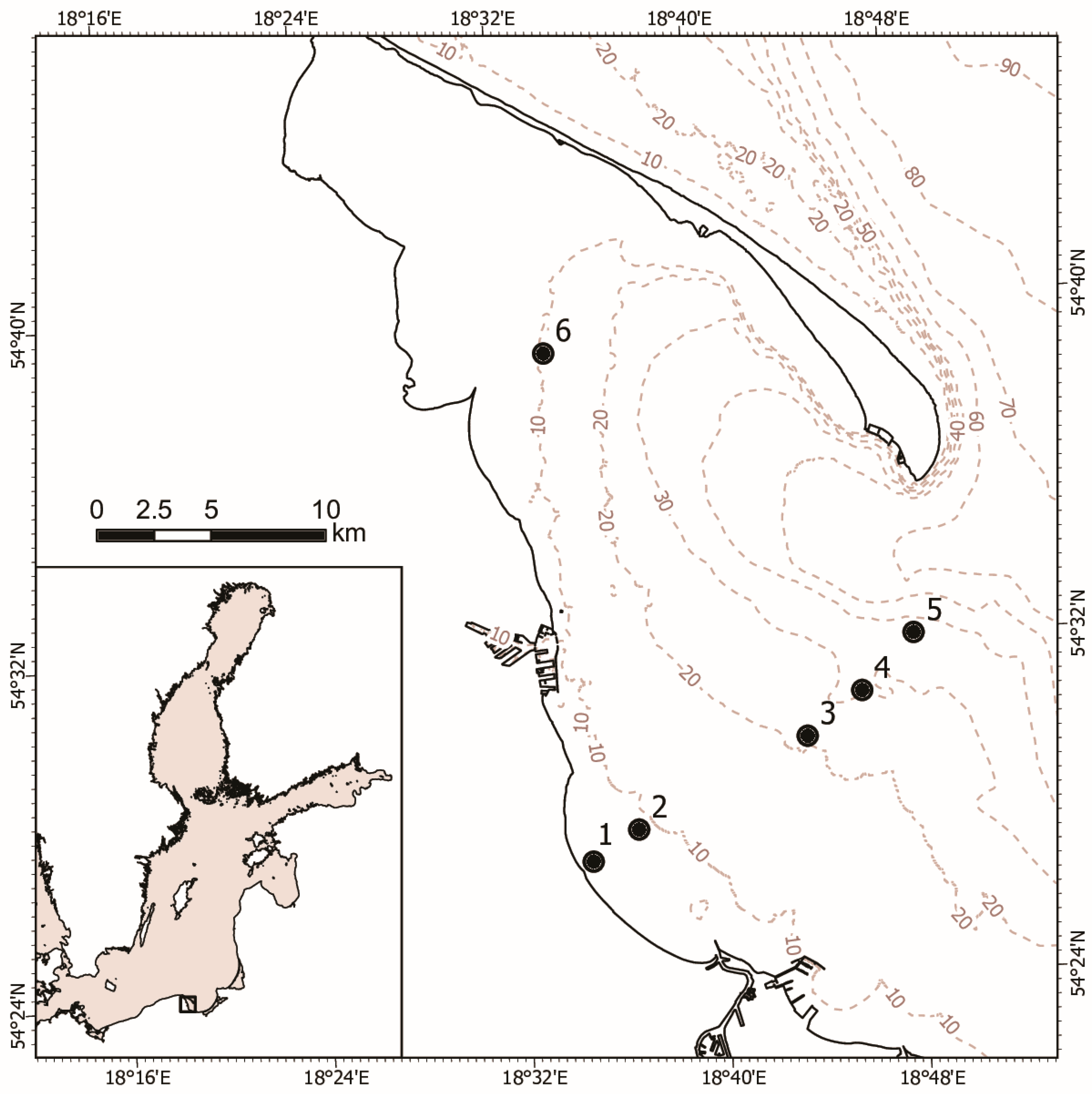
2.1. Study Area
2.2. Sampling
2.3. Model Data
2.4. Biomass and Abundance
2.5. Secondary Production
2.6. Mortality Rate
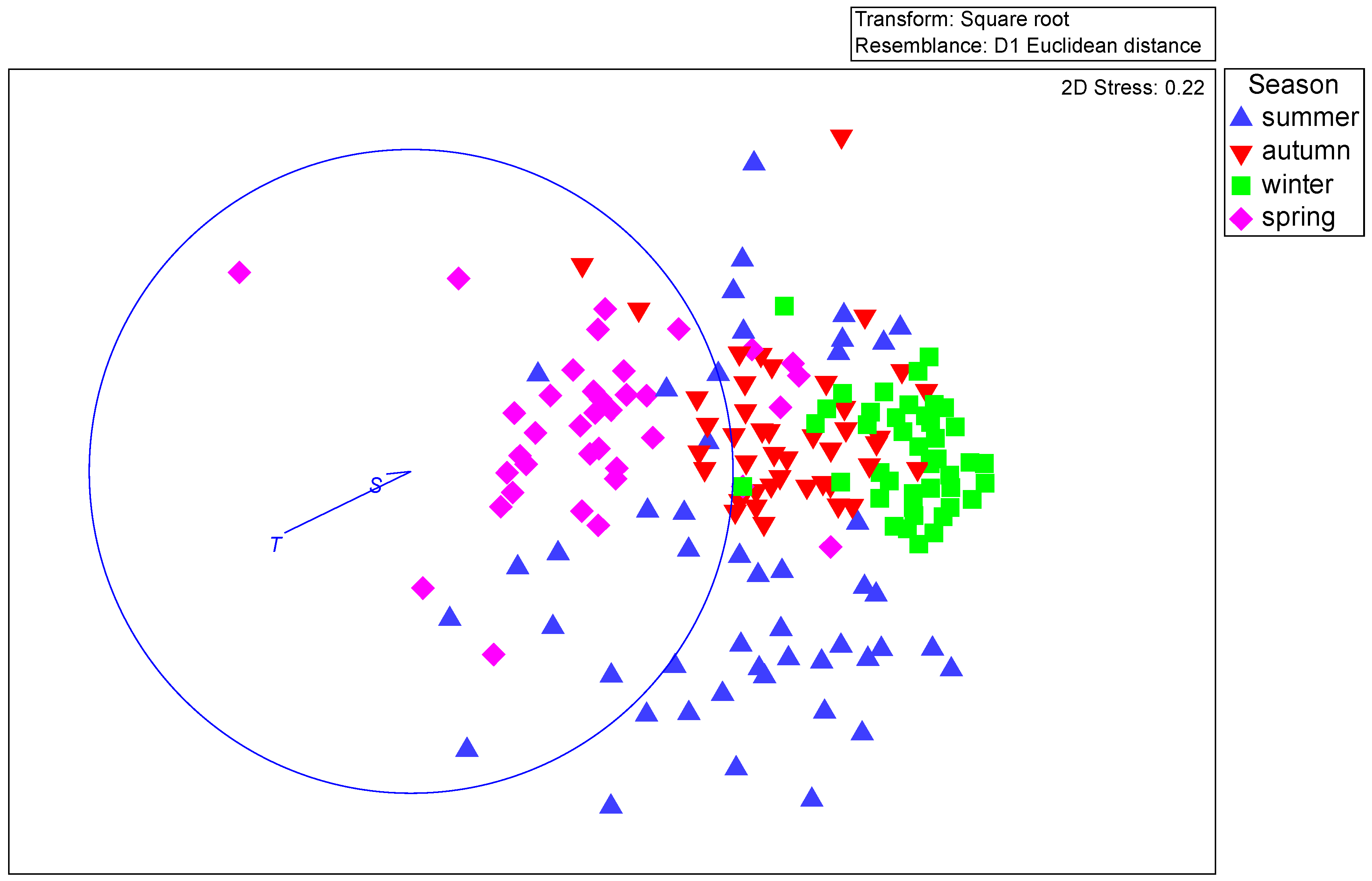
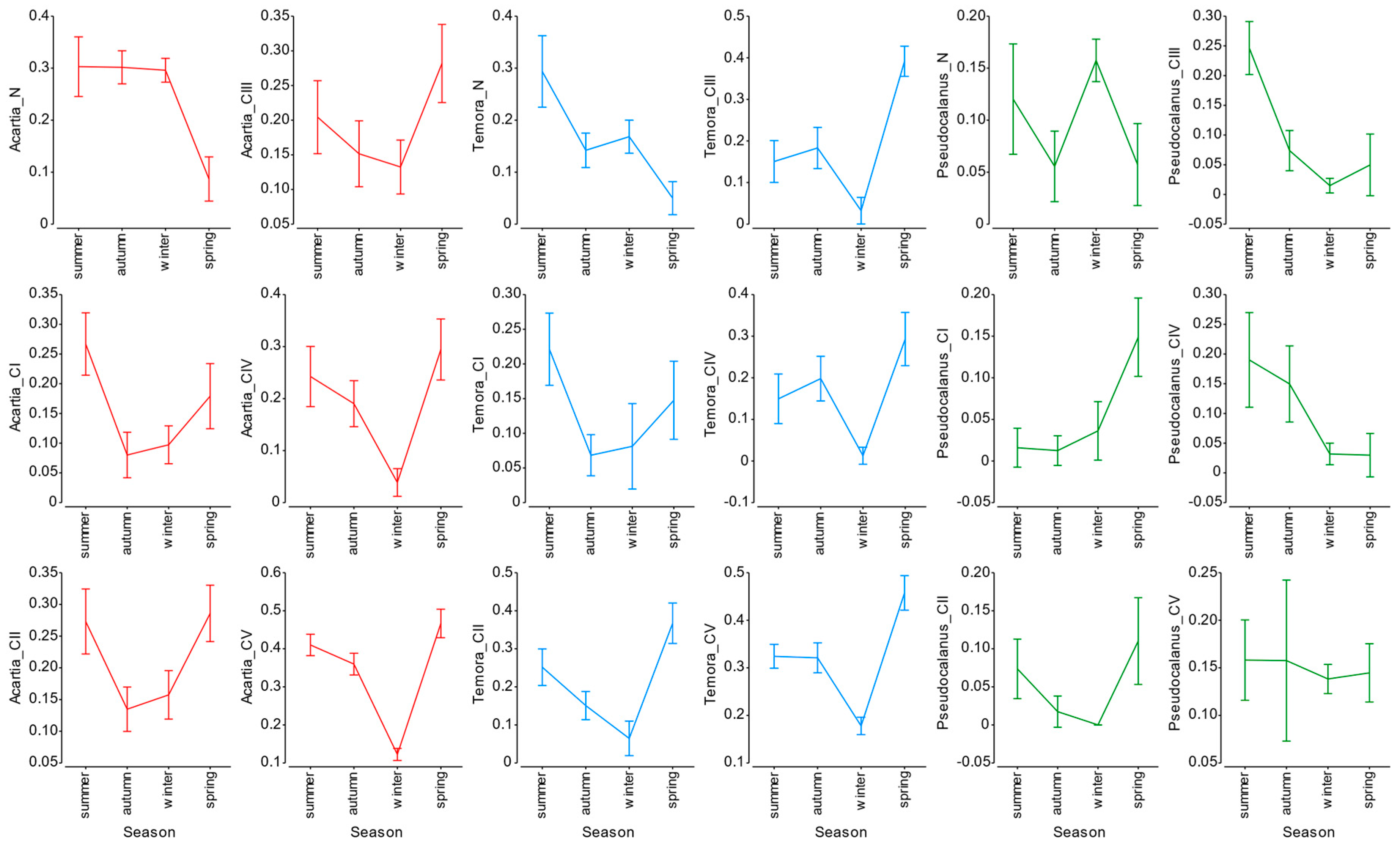
2.7. Statistical Analyses
3. Results
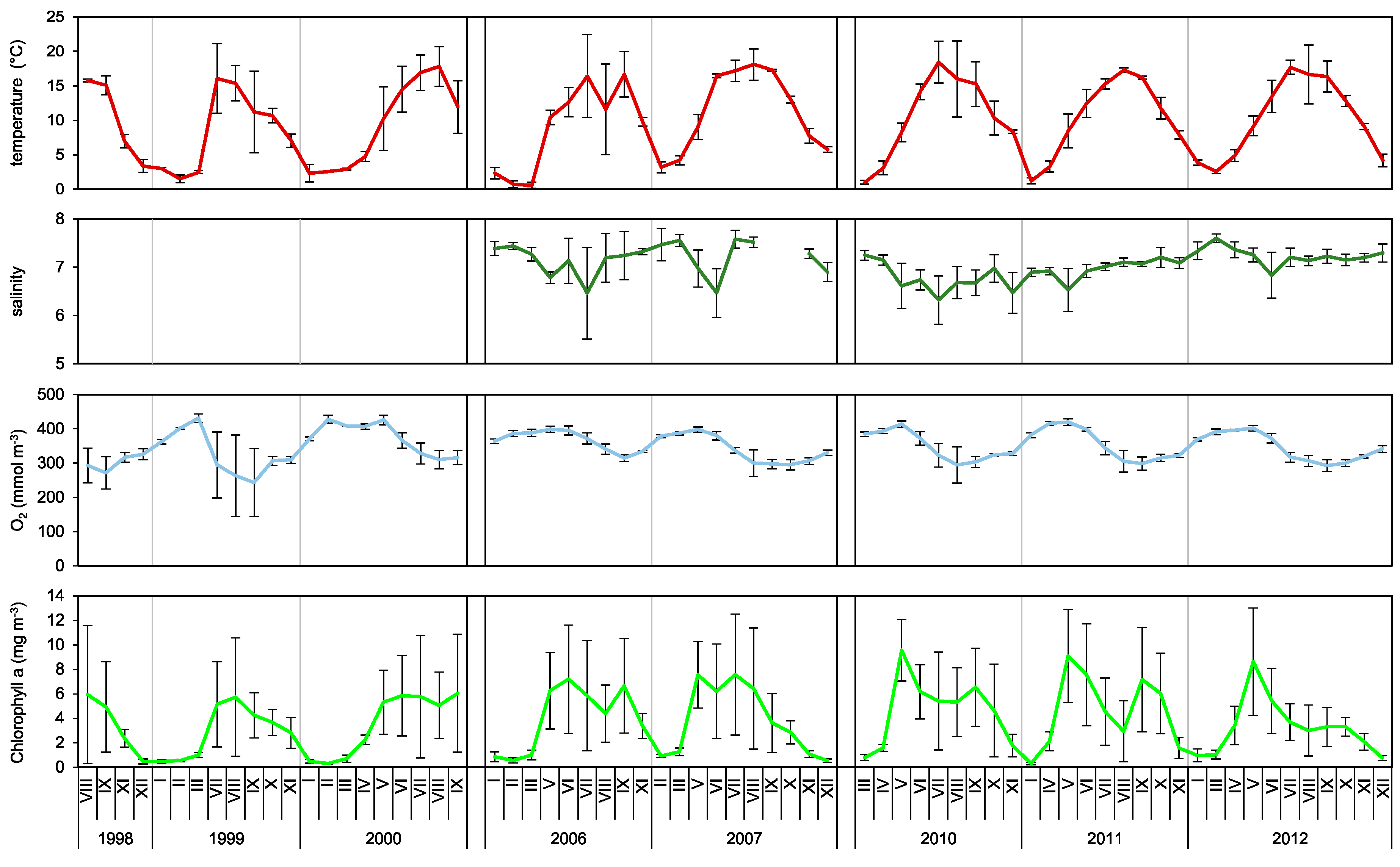
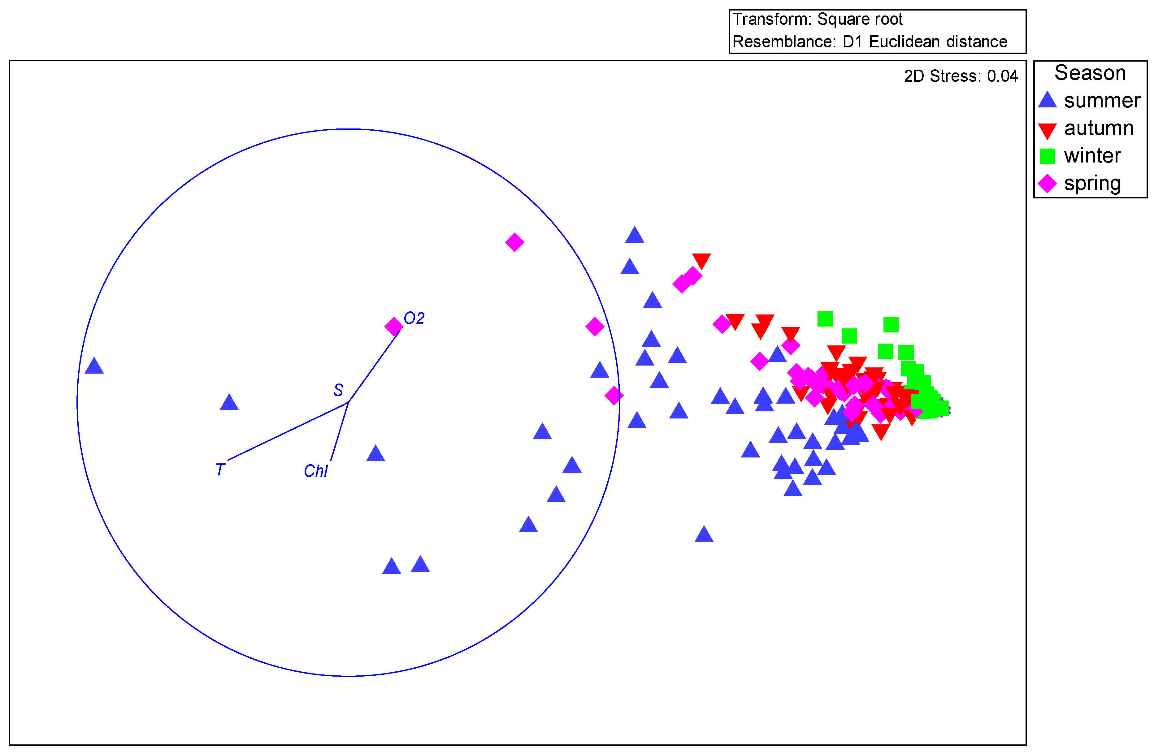
3.1. Hydrology
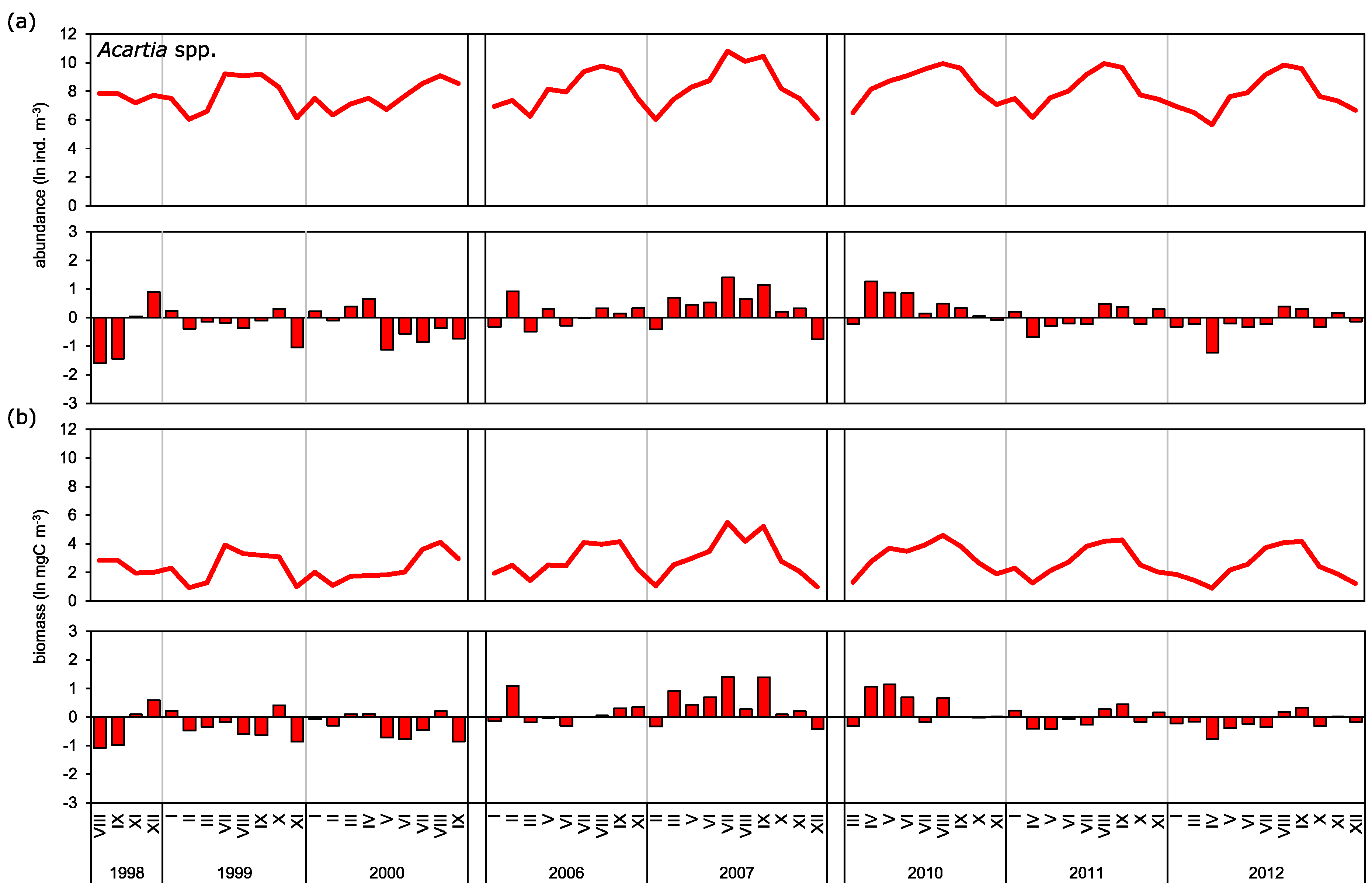
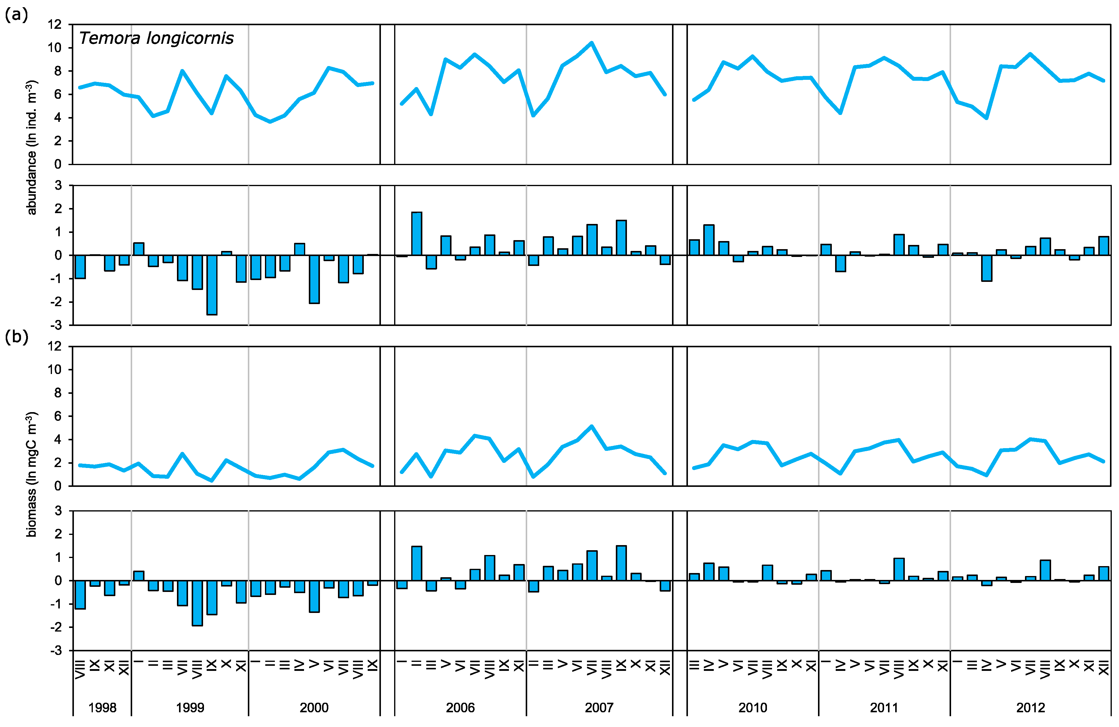
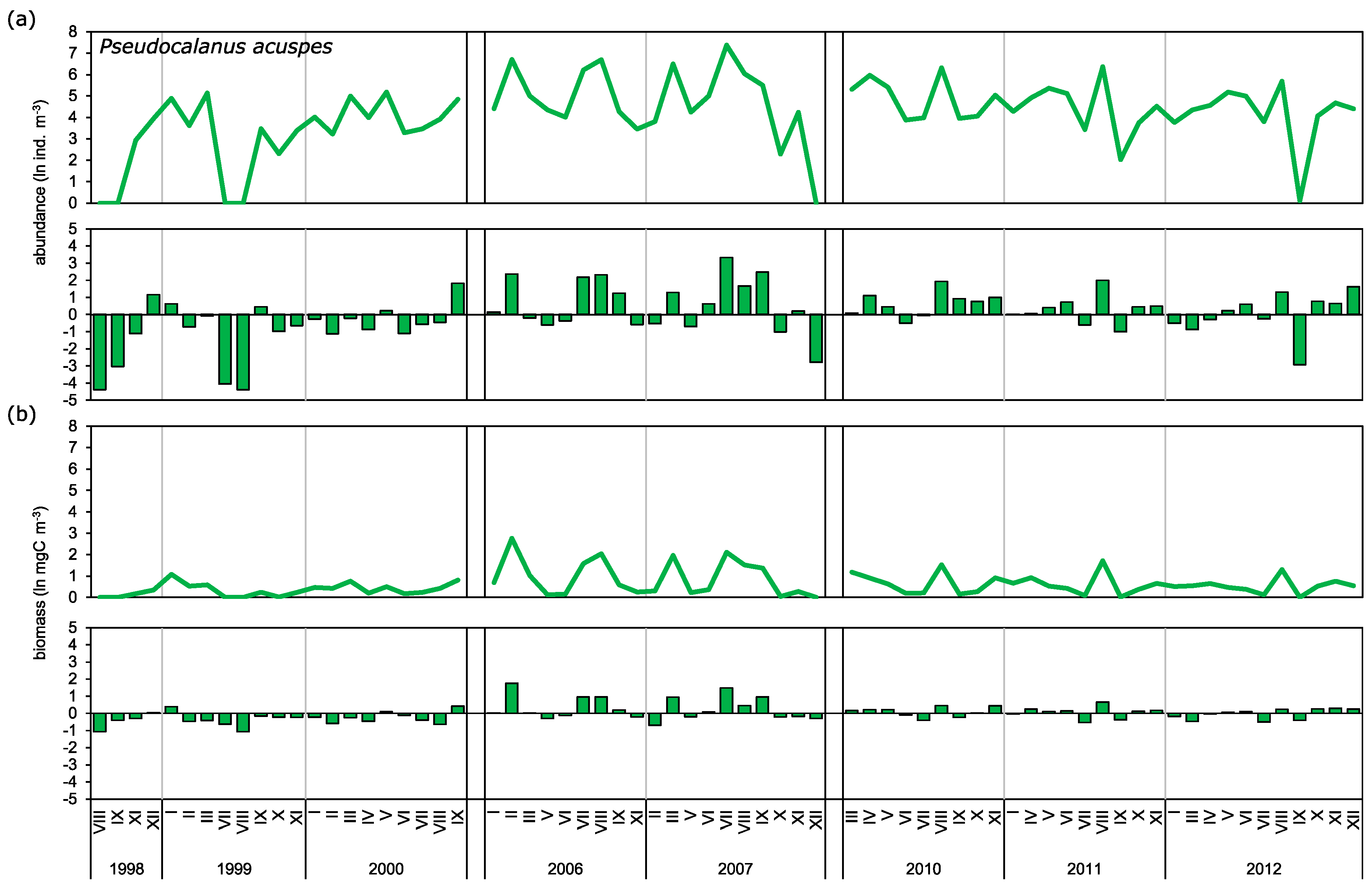
3.2. Abundance and Biomass Anomalies
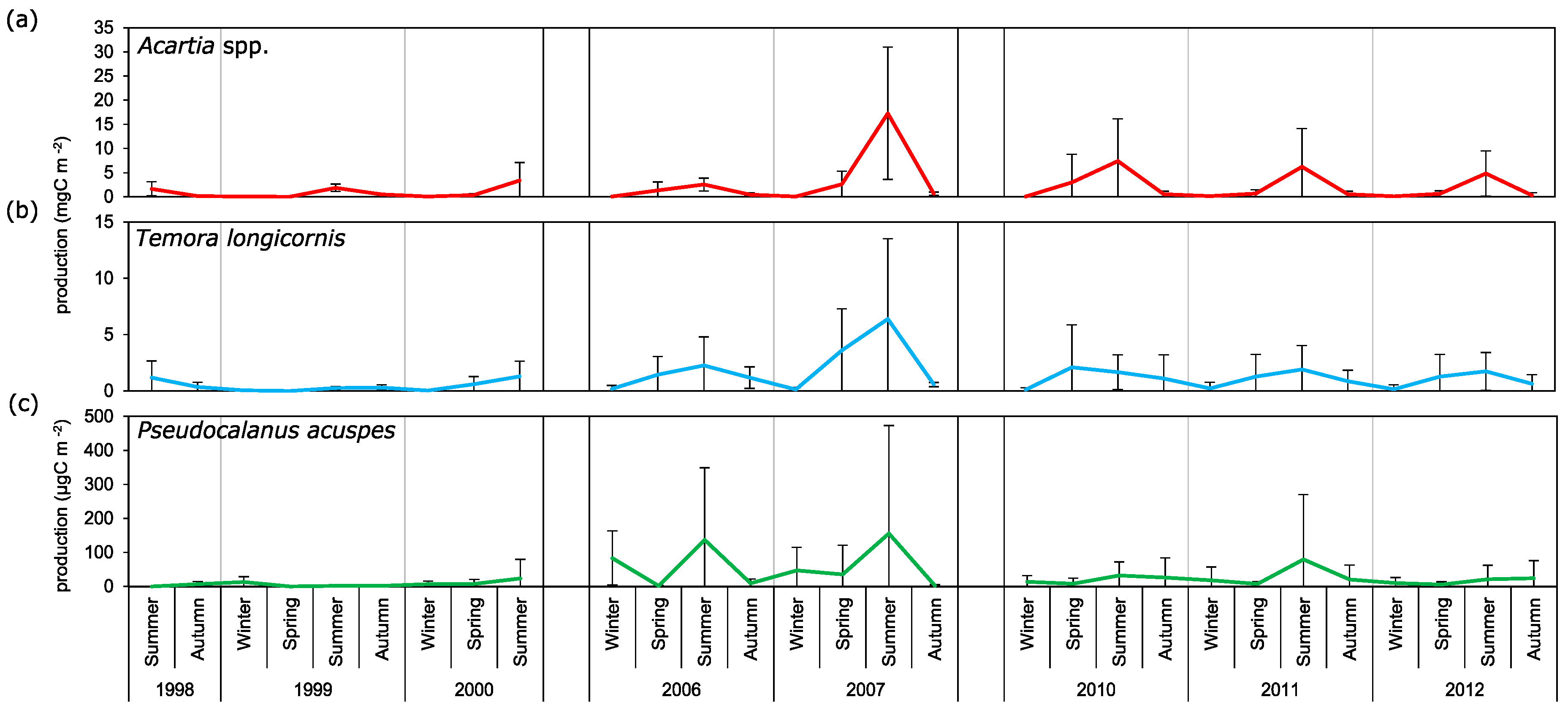
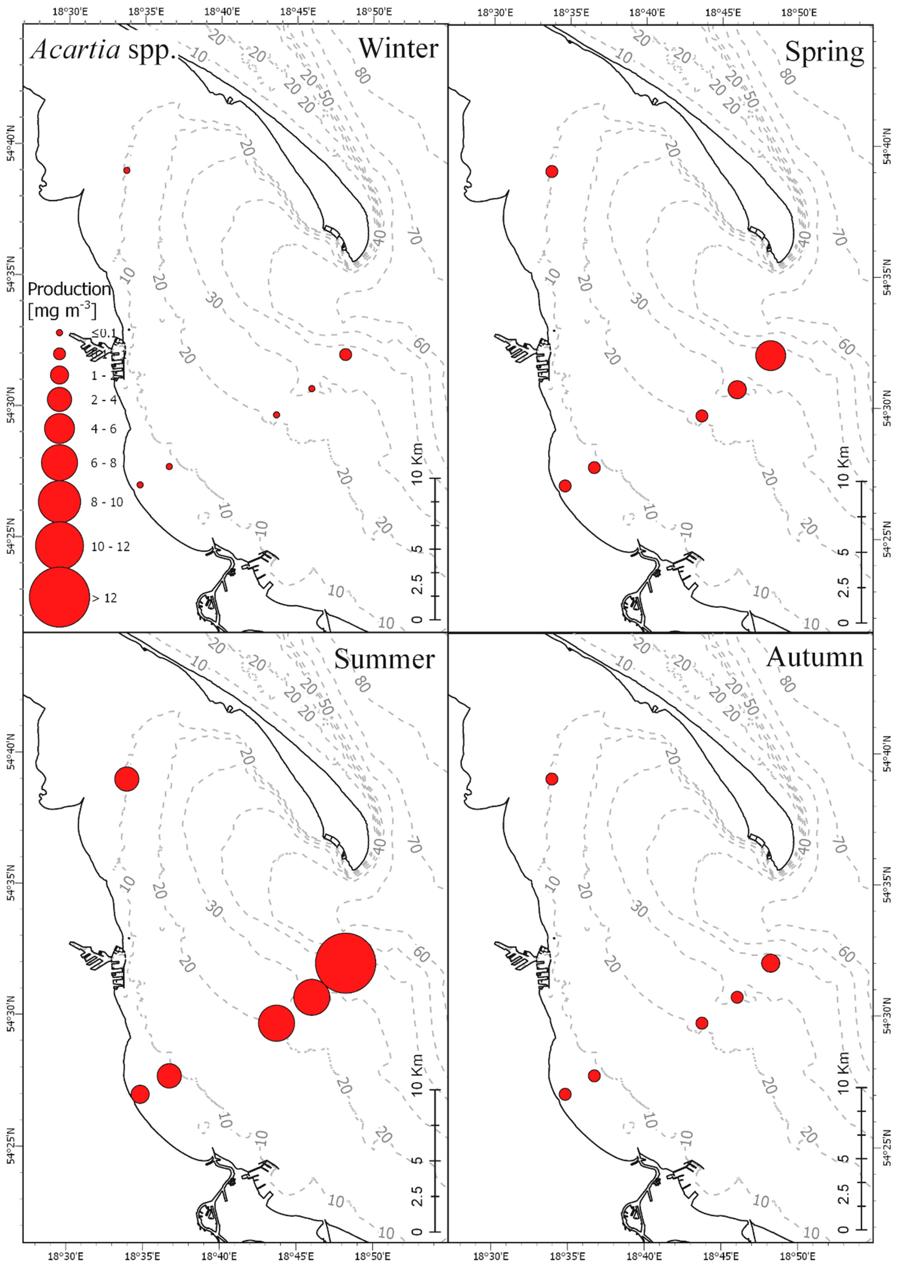
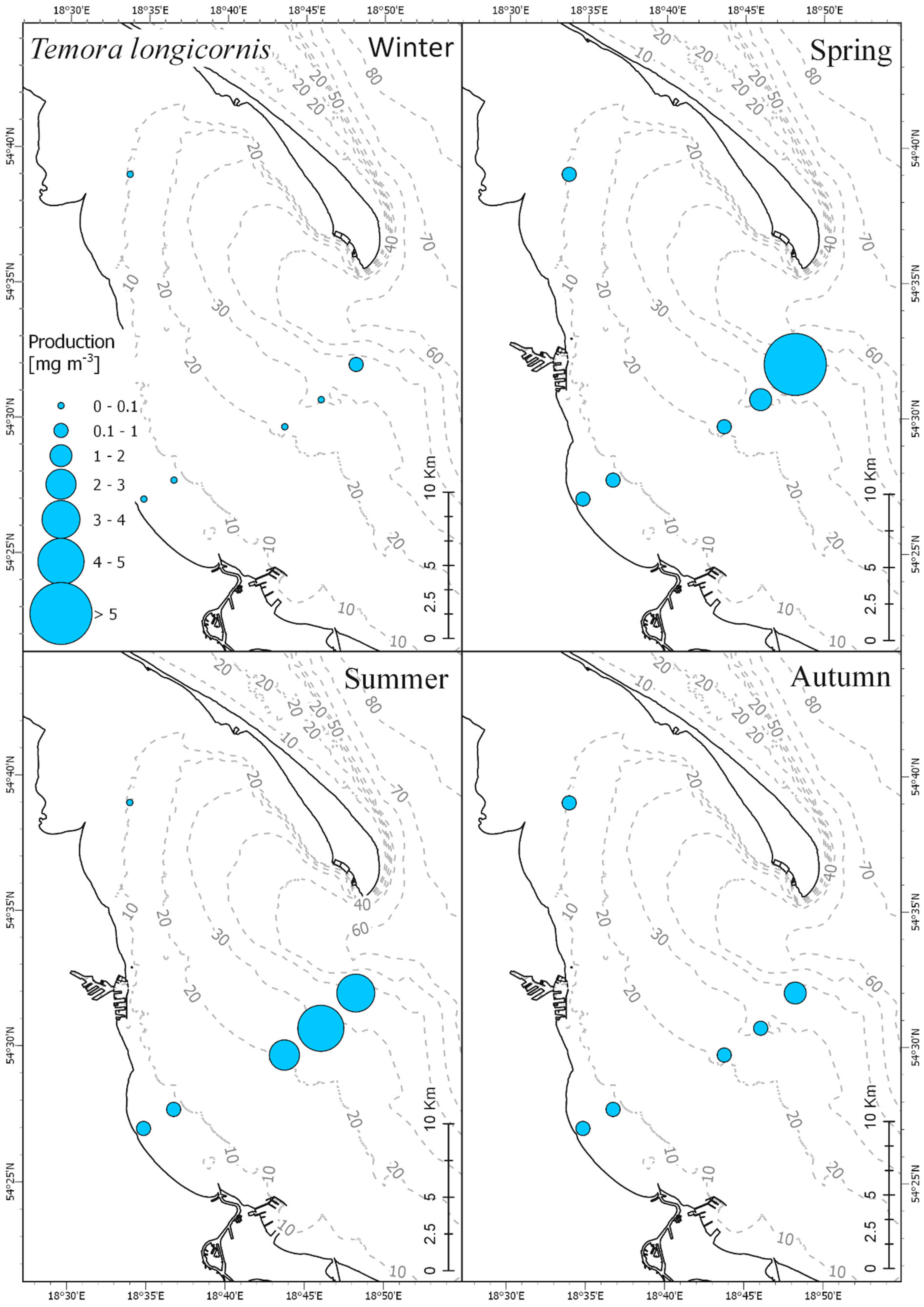
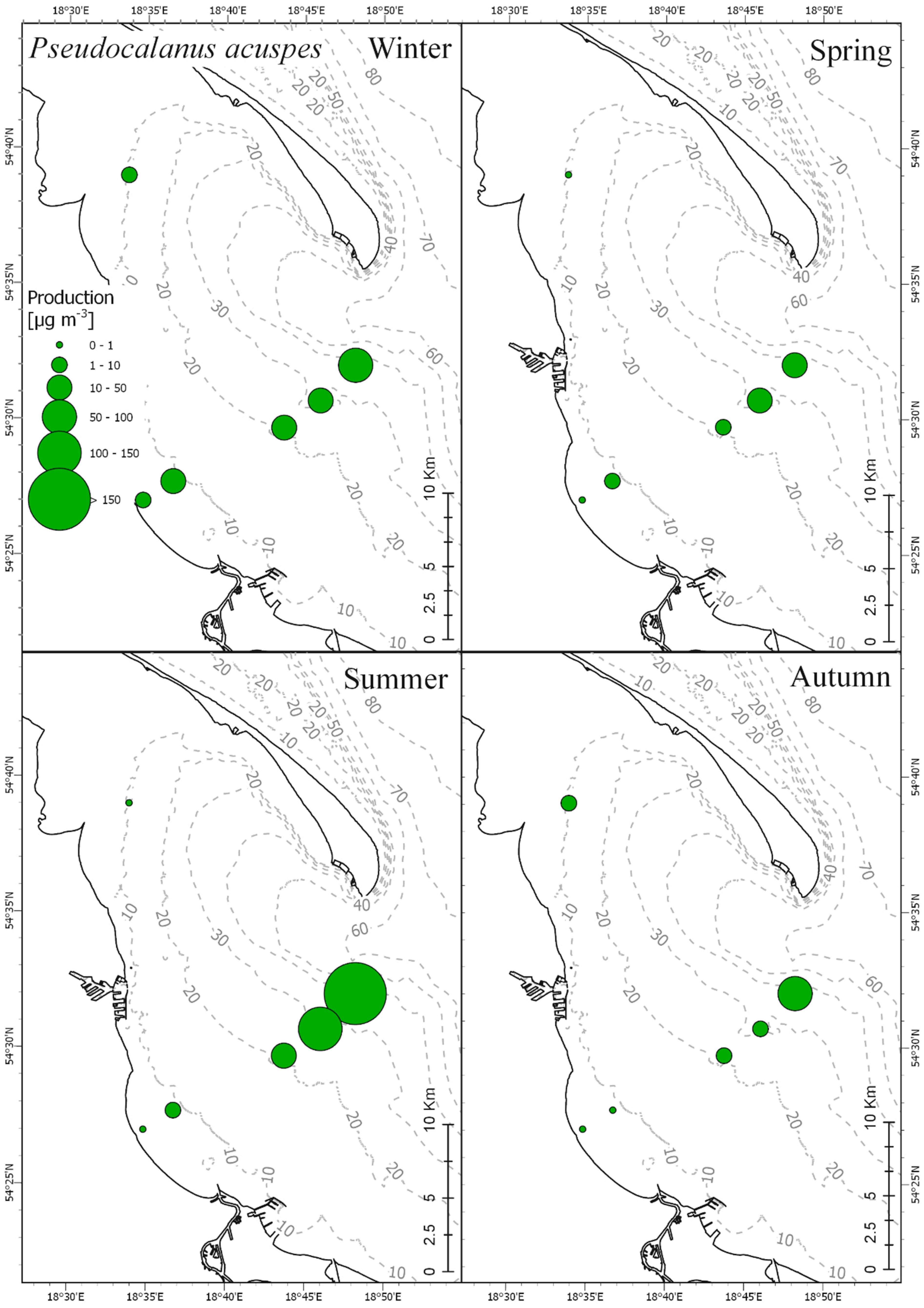
3.3. Secondary Production
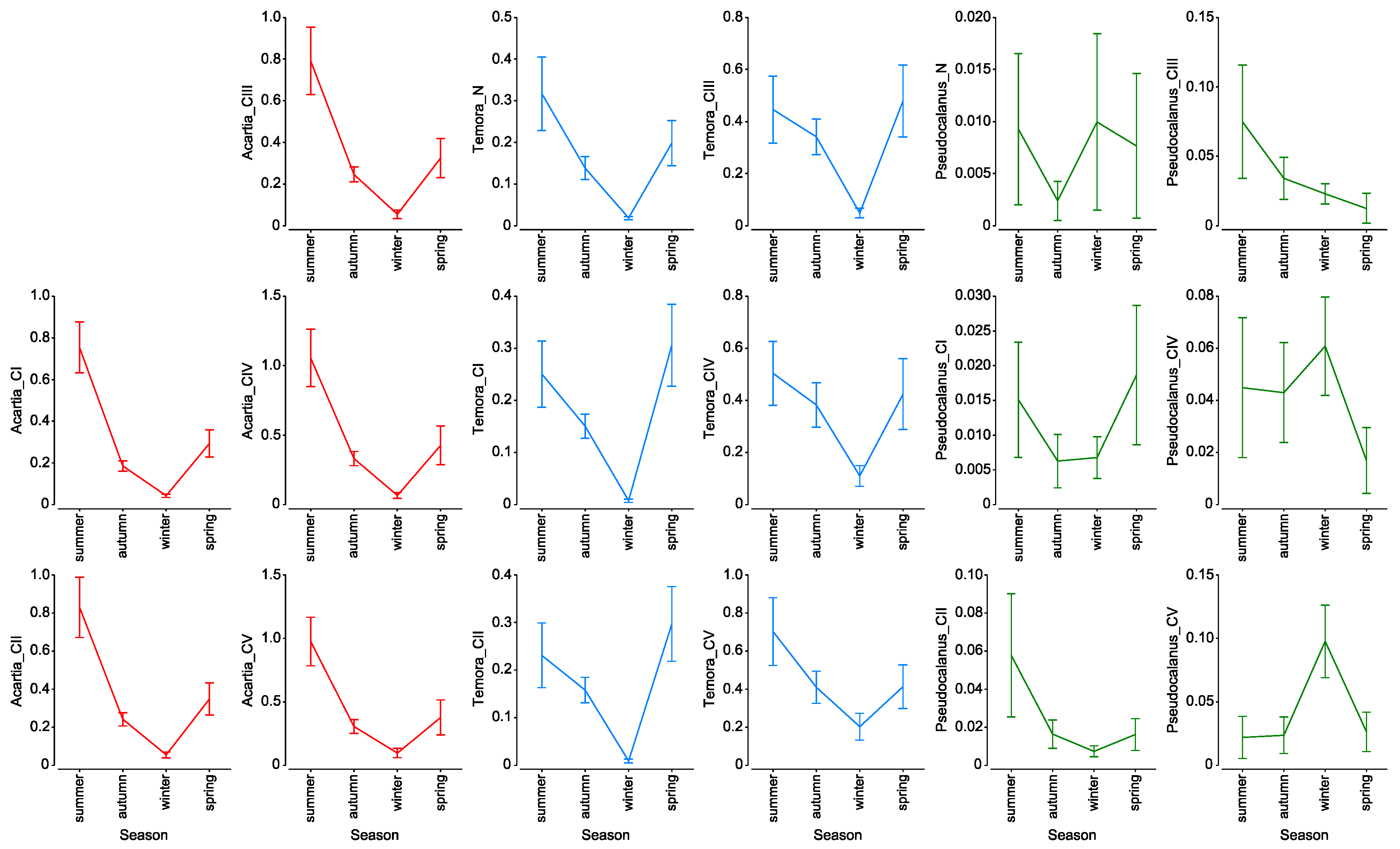
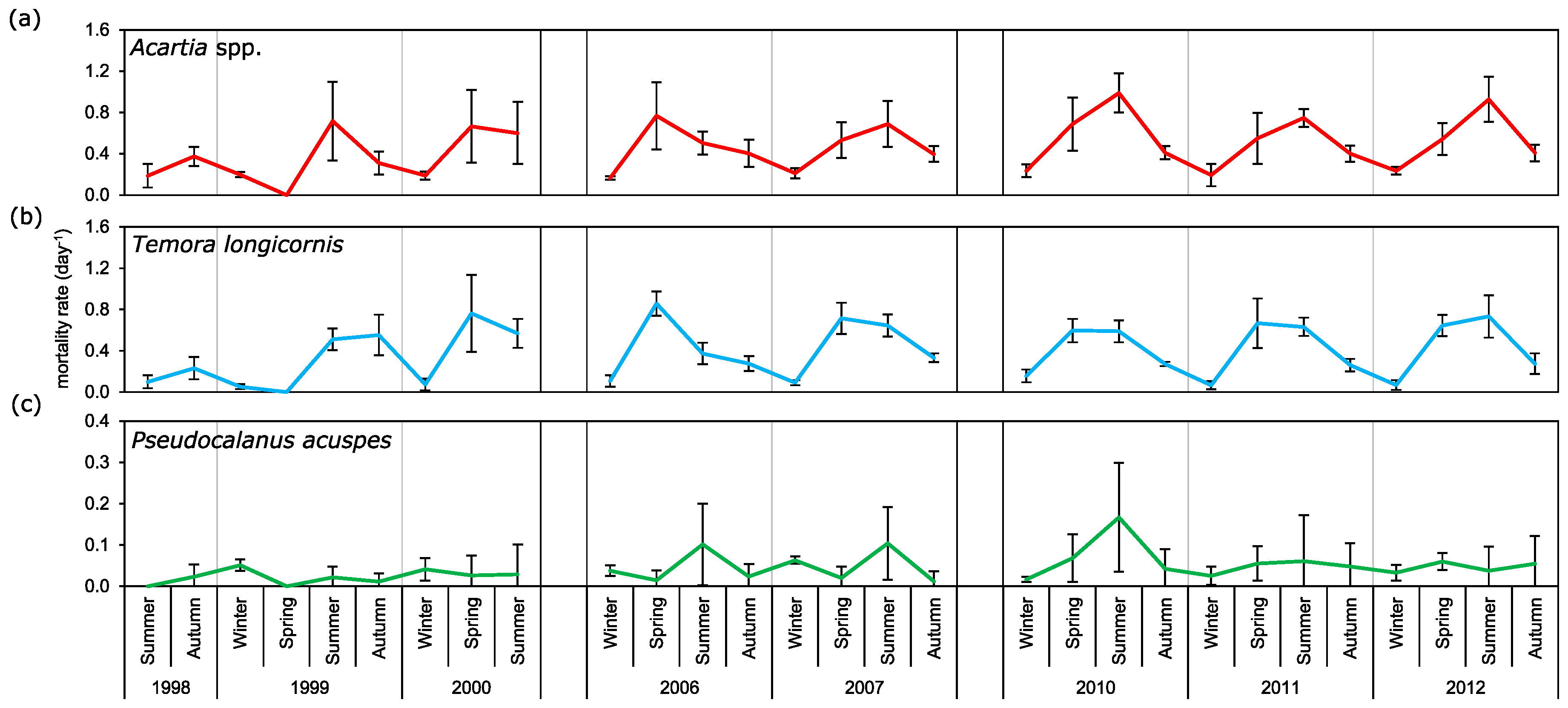
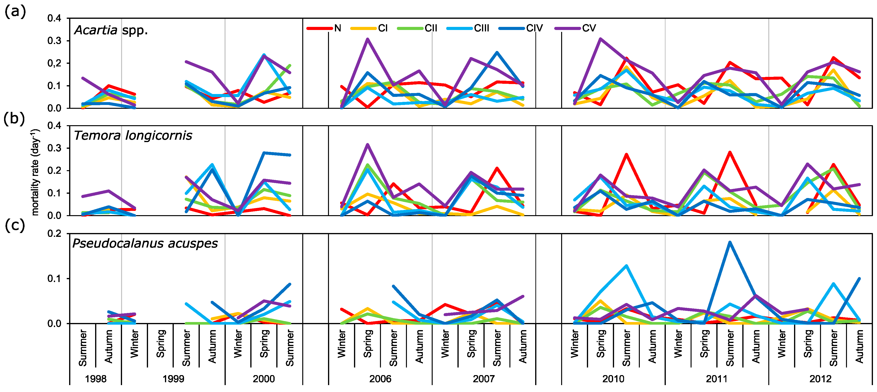
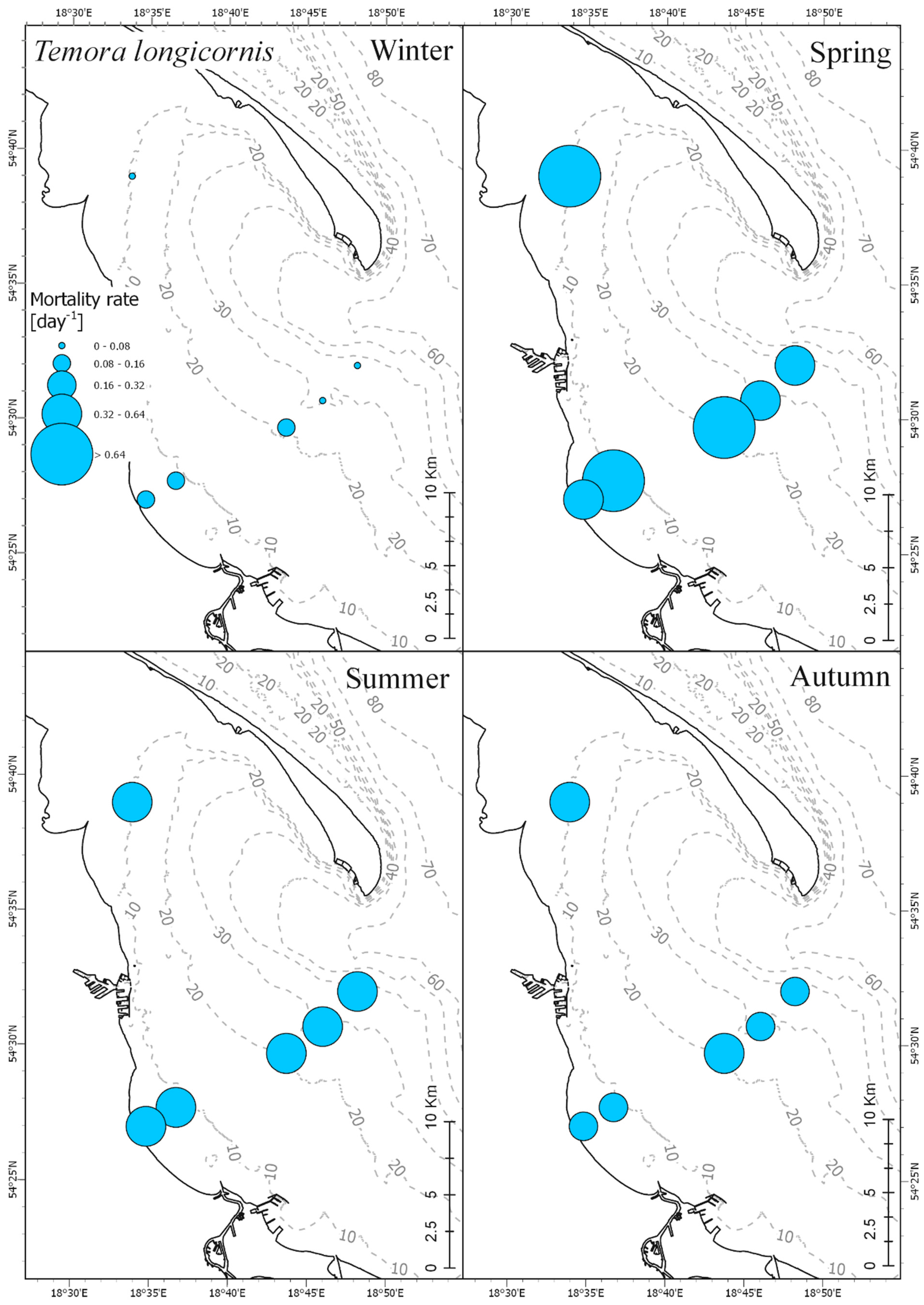
3.4. Mortality Rate
4. Discussion
Author Contributions
Funding
Acknowledgments
Conflicts of Interest
References
- Aksnes, D.L.; Ohman, M.D. A vertical life table approach to zooplankton mortality estimation. Limnol. Oceanogr. 1996, 41, 1461–1469. [Google Scholar] [CrossRef]
- Ohman, M.D.; Wood, S.N. Mortality estimation for planktonic copepods: Pseudocalanus newmani in a temperate fjord. Limnol. Oceanogr. 1996, 41, 126–135. [Google Scholar] [CrossRef]
- Dzierzbicka-Głowacka, L.; Kalarus, M.; Musialik-Koszarowska, M.; Lemieszek, A.; Żmijewska, M.I. Seasonal variability in the population dynamics of the main mesozooplankton species in the Gulf of Gdańsk (southern Baltic Sea): Production and mortality rates. Oceanologia 2015, 57, 78–85. [Google Scholar] [CrossRef]
- Corkett, C.J.; Zillioux, F.J. Studies on the effects of temperature on the egg laying of three species of calanoid copepods in the laboratory (Acartia tonsa, Temora longicornis and Pseudocalanus elongatus). Bull. Plankton Soc. Jpn. 1975, 21, 77–85. [Google Scholar]
- Paffenhöfer, G.A.; Harris, R.P. Feeding, growth, and reproduction of the marine planktonic copepod Pseudocalanus elongatus Boeck. J. Mar. Biol. Assoc. UK 1976, 56, 327–344. [Google Scholar] [CrossRef]
- Klein Breteler, W.C.M.; Fransz, H.G.; Gonzalez, S.R. Growth and development of four calanoid copepod species under experimental and natural conditions. Neth. J. Sea Res. 1982, 16, 195–207. [Google Scholar] [CrossRef]
- Koski, M.; Klein Breteler, W.C.M.; Schogt, N. Effect of food quality on rate of growth and development of the pelagic copepod Pseudocalanus elongatus (Copepoda, Calanoida). Mar. Ecol. Prog. Ser. 1998, 170, 169–187. [Google Scholar] [CrossRef]
- Koski, M.; Klein Breteler, W.C.M. Influence of diet on copepod survival in the laboratory. Mar. Ecol. Prog. Ser. 2003, 264, 73–82. [Google Scholar] [CrossRef][Green Version]
- Klein Breteler, W.C.M.; Schogt, N.; Rampen, S. Effect of diatom nutrient limitation on copepod development: Role of essential lipids. Mar. Ecol. Prog. Ser. 2005, 291, 125–133. [Google Scholar] [CrossRef]
- Dzierzbicka-Głowacka, L.; Lemieszek, A.; Żmijewska, M.I. Development and growth of Temora longicornis: Numerical simulations using laboratory culture data. Oceanologia 2011, 53, 137–161. [Google Scholar] [CrossRef]
- Kiørbe, T.; Johansen, K. Studies of a larval herring (Clupea harengus L.) patch in the Buchan area. IV. Zooplankton distribution and productivity in relation to hydrographic features. Dana 1986, 6, 37–51. [Google Scholar]
- Nielsen, T.G. Contribution of zooplankton grazing to the decline of a Ceratium bloom. Limnol. Oceanogr. 1991, 36, 1091–1106. [Google Scholar] [CrossRef]
- Kiørbe, T.; Nielsen, T.G. Regulation of zooplankton biomass and production in a temperate, coastal ecosystem. 1. Copepods. Limnol. Oceanogr. 1994, 39, 493–507. [Google Scholar] [CrossRef]
- Halsband, C.; Hirche, H.J. Reproductive cycles of dominant calanoid copepods in the North Sea. Mar. Ecol. Prog. Ser. 2001, 209, 219–229. [Google Scholar] [CrossRef]
- Eiane, K.; Ohman, M.D. Stage specific mortality of Calanus finmarchicus, Pseudocalanus elongatus and Oithona similis on Fladen Ground, North Sea, during a spring bloom. Mar. Ecol. Prog. Ser. 2004, 268, 183–193. [Google Scholar] [CrossRef]
- Dzierzbicka-Głowacka, L.; Kalarus, M.; Żmijewska, M.I. Interannual variability in the population dynamics of the main mesozooplankton species in the Gulf of Gdańsk (southern Baltic Sea): Seasonal and spatial distribution. Oceanologia 2013, 55, 409–434. [Google Scholar] [CrossRef][Green Version]
- Musialik-Koszarowska, M.; Dzierzbicka-Głowacka, L.; Kalarus, M.; Lemieszek, A.; Maruszak, P.; Żmijewska, M.I. Population dynamics of the main copepod species in the Gulf of Gdańsk (the southern Baltic Sea): Abundance, biomass and production rates. Oceanol. Hydrobiol. Stud. 2016, 45, 159–171. [Google Scholar] [CrossRef]
- Dzierzbicka-Głowacka, L. A numerical investigation of phytoplankton and Pseudocalanus elongatus dynamics in the spring bloom time in the Gdańsk Gulf. J. Mar. Syst. 2005, 53, 1–4, 19–36. [Google Scholar] [CrossRef]
- Dzierzbicka-Głowacka, L.; Bielecka, L.; Mudrak, S. Seasonal dynamics of Pseudocalanus minutus elongatus and Acartia spp. in the southern Baltic Sea (Gdańsk Deep)—Numerical simulations. Biogeosciences 2006, 3, 635–650. [Google Scholar] [CrossRef]
- Dzierzbicka-Głowacka, L.; Żmijewska, M.I.; Mudrak, S.; Jakacki, J.; Lemieszek, A. Population modelling of Acartia spp. in a water column ecosystem model for the South-Eastern Baltic Sea. Biogeosciences 2010, 7, 2247–2259. [Google Scholar] [CrossRef]
- Copernicus Marine Environment Monitoring Service’s (CMEMS). Available online: http://marine.copernicus.eu/documents/QUID/CMEMSBAL-QUID-003-012.pdf (accessed on 23 March 2019).
- HELCOM. Manual for Marine Monitoring in the COMBINE Programme of HELCOM. 2017. Available online: http://helcom.fi/action-areas/monitoring-and-assessment/manuals-and-guidelines/combine-manual/ (accessed on 20 February 2019).
- Hernroth, L. Recommendations on methods for marine biological studies in the Baltic Sea: Mesozooplankton Biomass Assessment. Balt. Mar. Biol. 1985, 10, 1–32. [Google Scholar]
- Edmondson, W.T.; Winberg, G.G. A Manual on Methods for the Assesment of Secondary Productivity in Freshwaters; Blackwell Scientific Publications: Oxford, UK, 1971; p. 358. [Google Scholar]
- Figiela, M.; Musialik-Koszarowska, M.; Nowicki, A.; Lemieszek, A.; Kalarus, M.; Druet, Cz. Long-term changes in the total development time of Copepoda species occurring in large numbers in the Southern Baltic Sea -numerical calculations. Oceanol. Hydrobiol. Stud. 2016, 45, 1–10. [Google Scholar] [CrossRef]
- Mullin, M.M. Production of zooplankton in the ocean: The present status and problems. Oceanogr. Mar. Biol. Rev. 1969, 7, 293–310. [Google Scholar]
- Clarke, K.R.; Gorley, R.N. PRIMER v7: User Manual/Tutorial; PRIMER-E: Plymouth, UK, 2015. [Google Scholar]
- Ter Braak, C.J.F.; Šmilauer, P. Canoco Reference Manual and User’s Guide: Software for Ordination, Version 5.0; Microcomputer Power: Ithaca, NY, USA, 2012. [Google Scholar]
- Richardson, A.J. In hot water: Zooplankton and climate change. ICES J. Mar. Sci. 2008, 65, 279–295. [Google Scholar] [CrossRef]
- Möllmann, C.; Kornilovs, G.; Sidrevics, L. Long-term dynamics of main mesozooplankton species in the central Baltic Sea. J. Plankton Res. 2000, 22, 2015–2038. [Google Scholar] [CrossRef]
- Gillooly, J. Effect of body size and temperature on generation time in zooplankton. J. Plankton Res. 2000, 22, 241–251. [Google Scholar] [CrossRef]
- Koski, M.; Jonasdottir, S.H.; Bagøien, E. Biological processes in the North Sea II. Vertical distribution and reproduction of neritic copepods in relation to environmental factors. J. Plankton Res. 2010, 51, 63–84. [Google Scholar] [CrossRef][Green Version]
- Escaravage, V.; Soetaert, K. Secondary production of the brackish copepod communities and their contribution to the carbon fluxes in the Westershelde estuary (The Netherlands). Hydrobiologia 1995, 311, 103–114. [Google Scholar] [CrossRef]
- Frost, B.W. A taxonomy of the marine calanoid copepod genus Pseudocalanus. Can. J. Zool. 1989, 67, 525–551. [Google Scholar] [CrossRef]
- Bucklin, A.; Frost, B.W.; Bradford-Grieve, J.; Allen, L.D.; Copley, N.J. Molecular systematic and phylogenetic assessment of 34 calanoid copepod species of the Calanidae and Clausocalanidae. Mar. Biol. 2003, 142, 333–343. [Google Scholar] [CrossRef]
- Renz, J.; Hirche, H.J. Life cycle of Pseudocalanus acuspes Giesbrecht (Copepoda, Calanoida) in the Central Baltic Sea: I. Seasonal and spatial distribution. Mar. Biol. 2006, 148, 567–580. [Google Scholar] [CrossRef]
- Musialik-Koszarowska, M.; Dzierzbicka-Głowacka, L.; Weydmann, A. Influence of environmental factors on the population dynamics of key zooplankton species in the Gulf of Gdańsk (Southern Baltic Sea). Oceanologia 2019, 177, 1–9. [Google Scholar] [CrossRef]
- Hall, C.J.; Burns, C.W. Effects of salinity and temperature on survival and reproduction of Boeckella hamata (Copepoda: Calanoida) from a Periodically Brackish Lake. J. Plankton Res. 2001, 23, 97–104. [Google Scholar] [CrossRef]
- Holste, L.; St. John, M.A.; Peck, M.A. The effects of temperature and salinity on reproductive success of Temora longicornis in the Baltic Sea: A copepod coping with a tough situation. Mar. Biol. 2009, 156, 527–540. [Google Scholar] [CrossRef]
- Nagaraj, M. Combined effects of temperature and salinity on the development of the copepod Eurytemora affinis. Aquaculture 1992, 103, 65–71. [Google Scholar] [CrossRef]
- Bossicart, M. Population Dynamics of Copepods in the Southern Bight of the North Sea (1977–1979), Use of a Multicohort Model to Derive Biological Parameters; Laboratorium voor Ekologie en Systematiek, Vrije Universiteit: Brussel, Belgium, 1980; pp. 171–182. [Google Scholar]
- Evans, F. Seasonal density and production estimates of the commoner planktonic copepods of Northhumberland coastal waters. Est. Coast. Mar. Sci. 1977, 5, 233–241. [Google Scholar] [CrossRef]
- Renz, J. Life Cycle and Population Dynamics of the Calanoid Copepod Pseudocalanus spp. in the Baltic Sea and North Sea. Ph.D. Thesis, University Bremen, Bremen, Germany, 2006. [Google Scholar]
- Renz, J.; Mengedoht, D.; Hirche, H.J. Reproduction, growth and secondary production of Pseudocalanus elongatus Boeck (Copepoda, Calanoida) in the southern North Sea. J. Plankton Res. 2008, 30, 511–528. [Google Scholar] [CrossRef]
- Fransz, H.G.; Miquel, J.C.; Gonzalez, S.R. Mesozooplankton composition, biomass and vertical distribution, and copepod production in the stratified Central North Sea. Neth. J. Sea Res. 1984, 18, 82–96. [Google Scholar] [CrossRef]
- The BACC II, Author Team. Second Assessment of Climate Change for the Baltic Sea Basin. Regional Climate Studies; Springer: Berlin/Heidelberg, Germany, 2008; pp. 1–22. Available online: http://dx.doi.org/10.1007/978-3-319-16006-1 (accessed on 18 January 2019).
- Allen, J.L.; Anderson, D.; Burford, M.; Dyhrman, S.; Flynn, K.; Gilbert, P.M.; Grane’li, E.; Heil, C.; Sellner, K.; Smayda, T.; et al. Global Ecology and Oceanography of Harmful Algal Blooms in Eutrophic Systems; GEOMAP report 4; IOC: Paris, France; SCOR: Baltimore, MD, USA, 2006; pp. 1–74. [Google Scholar]
- Ohman, M.D.; Wood, S.N. The inevitability of mortality. ICES J. Mar. Sci. 1995, 52, 517–522. [Google Scholar] [CrossRef]
- Cushing, D.H. The possible density-dependence of larval mortality and adult mortality in fishes. In The Early Life History of Fish; Blaxter, J.H.S., Ed.; Springer: New York, NY, USA; Heidelberg/Berlin, Germany, 1974; pp. 103–111. [Google Scholar]
- Peterson, I.; Wróblewski, S.J. Mortality rate of fishes in the pelagic ecosystem. Can. J. Fish. Aquat. Sci. 1984, 41, 1117–1120. [Google Scholar] [CrossRef]
- Thor, P.; Nielsen, T.G.; Tiselius, P. Mortality rates of epipelagic copepods in the post-spring bloom period in Disko Bay, western Greenland. Mar. Ecol. Prog. Ser. 2008, 359, 151–160. [Google Scholar] [CrossRef]
- Plourde, S.; Pepin, P.; Head, E.J.H. Long-term seasonal and spatial patterns in mortality and survival of Calanus finmarchicus across the Atlantic Zone Monitoring Programme region, northwest Atlantic. ICES J. Mar. Sci. 2009, 66, 1942–1958. [Google Scholar] [CrossRef]
- Maud, J.L.; Atkinson, A.; Hirst, A.G.; Lindeque, P.K.; Widdicombe, C.L.; Harmer, R.A.; McEvoy, A.J.; Cummings, D.G. How does Calanus helgolandicus maintain its population in a variable environment? Analysis of a 25-year time series from the English Channel. Prog. Oceanogr. 2015, 137, 513–523. [Google Scholar] [CrossRef]
- Ohman, M.D.; Durbin, E.G.; Runge, J.A.; Sullivan, B.K.; Field, D.B. Relationship of predation potential to mortality of Calanus finmarchicus on Georges Bank, northwest Atlantic. Limnol. Oceanogr. 2008, 53, 1643–1655. [Google Scholar] [CrossRef]
- Hernroth, L.; Grondahl, F. On the Biology of Aurelia aurita. Ophelia 1993, 22, 189–199. [Google Scholar] [CrossRef]
- Rodriguez-Grana, L.; Calliari, D.; Tiselius, P.; Hansen, B.W.; Skold, H.N. Gender-specific ageing and non-Mendelian inheritance of oxidative damage in marine copepods. Mar. Ecol. Prog. Ser. 2010, 401, 1–13. [Google Scholar] [CrossRef]
- Kimmerer, W.J.; McKinnon, A.D. High mortality in a copepod population caused by a parasitic dinoflagellate. Mar. Biol. 1990, 107, 449–452. [Google Scholar] [CrossRef]
- Wendt, I.; Backhaus, T.; Blanck, H.; Arrhenius, Å. The toxicity of the three antifouling biocides DCOIT, TPBP and medetomidine to the marine pelagic copepod Acartia tonsa. Ecotoxicology 2016, 25, 871–879. [Google Scholar] [CrossRef]
- Tang, K.W.; Gladyshev, M.I.; Dubovskaya, O.P.; Kirillin, G.; Grossart, H.-P. Zooplankton carcasses and non-predatory mortality in freshwater and inland sea environments. J. Plankton Res. 2014, 36, 597–612. [Google Scholar] [CrossRef]
- Hirst, A.G.; Kiorboe, T. Mortality of marine planktonic copepods: Global rates and patterns. Mar. Ecol. Prog. Ser. 2002, 230, 195–209. [Google Scholar] [CrossRef]
- Ackefors, H. Ecological zooplankton investigations in the Baltic proper 1963–1965. Inst. Mar. Res. Lysekil Ser. Biol. Rep. 1969, 18, 1–139. [Google Scholar]
- Siudziński, K. Zooplankton of Gdańsk Bay; Studies and Materials of the Marine Fisheries Institute: Gdynia, Poland, 1977; Volume 18A, pp. 1–111. [Google Scholar]


| RMS Error | 0–5 m | 5–30 m | 30–80 m |
|---|---|---|---|
| Dissolved oxygen (mmol m−3) | 19 | 38 | 51 |
| Chlorophyll a (mg m−3) | 5 | 3 | 0.9 |
| Month | Acartia spp. | T. longicornis | P. acuspes |
|---|---|---|---|
| January | 7.28 ± 0.30 | 5.26 ± 0.63 | 4.27 ± 0.43 |
| February | 6.45 ± 0.63 | 4.62 ± 1.26 | 4.34 ± 1.60 |
| March | 6.74 ± 0.44 | 4.87 ± 0.62 | 5.21 ± 0.71 |
| April | 6.88 ± 1.15 | 5.09 ± 1.11 | 4.86 ± 0.83 |
| May | 7.85 ± 0.70 | 8.19 ± 1.04 | 4.95 ± 0.52 |
| June | 8.23 ± 0.56 | 8.49 ± 0.41 | 4.38 ± 0.76 |
| July | 9.41 ± 0.69 | 9.10 ± 0.87 | 4.04 ± 2.34 |
| August | 9.46 ± 0.75 | 7.58 ± 0.93 | 4.38 ± 2.83 |
| September | 9.30 ± 0.78 | 6.94 ± 1.14 | 3.02 ± 2.10 |
| October | 7.98 ± 0.27 | 7.41 ± 0.15 | 3.29 ± 0.92 |
| November | 7.18 ± 0.49 | 7.46 ± 0.66 | 4.04 ± 0.78 |
| December | 6.83 ± 0.83 | 6.39 ± 0.69 | 2.78 ± 2.42 |
| Month | Acartia spp. | T. longicornis | P. acuspes |
|---|---|---|---|
| January | 2.08 ± 0.21 | 1.54 ± 0.48 | 0.69 ± 0.24 |
| February | 1.39 ± 0.74 | 1.29 ± 0.98 | 1.01 ± 1.17 |
| March | 1.62 ± 0.47 | 1.26 ± 0.44 | 1.01 ± 0.52 |
| April | 1.67 ± 0.80 | 1.13 ± 0.53 | 0.67 ± 0.33 |
| May | 2.55 ± 0.68 | 2.94 ± 0.69 | 0.41 ± 0.20 |
| June | 2.79 ± 0.59 | 3.21 ± 0.38 | 0.29 ± 0.12 |
| July | 4.08 ± 0.64 | 3.85 ± 0.77 | 0.62 ± 0.85 |
| August | 3.91 ± 0.56 | 3.01 ± 1.13 | 1.07 ± 0.80 |
| September | 3.83 ± 0.80 | 1.92 ± 0.80 | 0.40 ± 0.49 |
| October | 2.69 ± 0.27 | 2.45 ± 0.21 | 0.25 ± 0.21 |
| November | 1.87 ± 0.40 | 2.50 ± 0.58 | 0.47 ± 0.30 |
| December | 1.40 ± 0.53 | 1.52 ± 0.53 | 0.30 ± 0.28 |
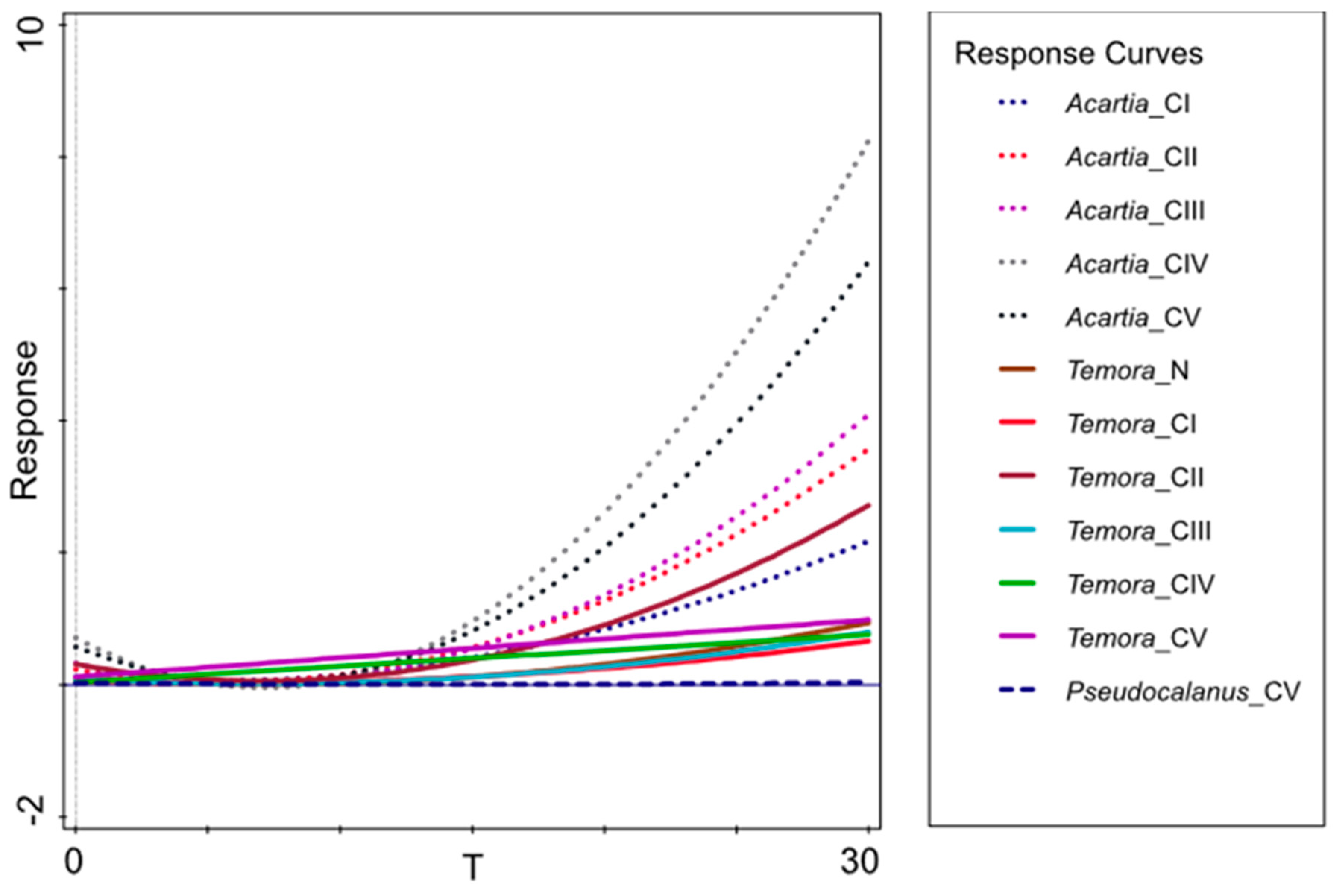
| Predictors | T | |||
| Distribution | normal | |||
| Link function | identity | |||
| GLM fitted for 12 response variables: | ||||
| Developmental stages | Type | R2[%] | F | p |
| Acartia spp._CI | quadratic | 18.4 | 18.4 | <0.00001 |
| Acartia spp._CII | quadratic | 1.0 | 17.4 | <0.00001 |
| Acartia spp._CIII | quadratic | 20.5 | 21.0 | <0.00001 |
| Acartia spp._CIV | quadratic | 24.6 | 26.6 | <0.00001 |
| Acartia spp._CV | quadratic | 20.9 | 21.5 | <0.00001 |
| Temora longicornis_N | quadratic | 19.5 | 19.8 | <0.00001 |
| Temora longicornis_CI | quadratic | 12.2 | 11.3 | 0.00002 |
| Temora longicornis_CII | quadratic | 15.0 | 14.3 | <0.00001 |
| Temora longicornis_CIII | quadratic | 14.0 | 13.3 | <0.00001 |
| Temora longicornis_CIV | linear | 5.5 | 9.6 | 0.00229 |
| Temora longicornis_CV | linear | 4.3 | 7.4 | 0.00732 |
| Pseudocalanus acuspes_CV | quadratic | 8.3 | 7.4 | 0.00086 |
| Predictors | T | |||
| Distribution | normal | |||
| Link function | identity | |||
| GLM fitted for 11 response variables: | ||||
| Developmental stages | Type | R2[%] | F | p |
| Acartia spp._CI | linear | 5.1 | 8.9 | 0.00331 |
| Acartia spp._CII | linear | 4.1 | 7.1 | 0.00868 |
| Acartia spp._CIV | linear | 11.5 | 21.3 | <0.00001 |
| Acartia spp._CV | quadratic | 20.3 | 20.7 | <0.00001 |
| Temora longicornis_N | linear | 5.4 | 9.3 | 0.00266 |
| Temora longicornis_CI | linear | 8.6 | 15.5 | 0.00012 |
| Temora longicornis_CII | linear | 5.6 | 9.8 | 0.00206 |
| Temora longicornis_CIII | linear | 4.5 | 7.7 | 0.00617 |
| Temora longicornis_CIV | linear | 4.0 | 6.9 | 0.00946 |
| Temora longicornis_CV | quadratic | 8.6 | 7.7 | 0.00064 |
| Pseudocalanus acuspes_CV | linear | 4.8 | 8.2 | 0.00478 |
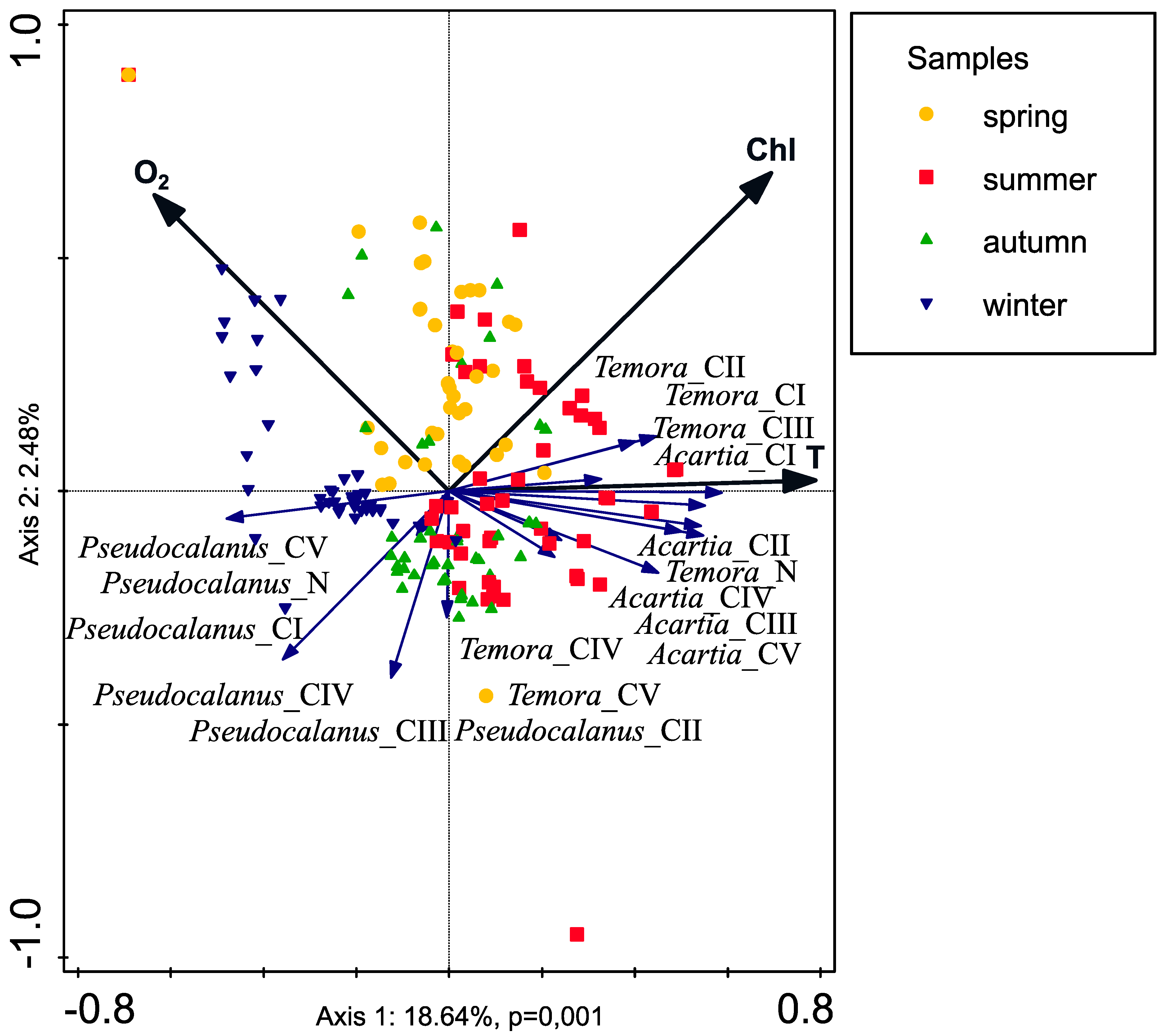
| Name | Explains % | pseudo-F | p |
|---|---|---|---|
| Temperature (T) | 11.8 | 15.6 | 0.001 |
| Dissolved oxygen (O2) | 5.0 | 7.0 | 0.002 |
| Chlorophyll a | 4.5 | 6.6 | 0.005 |
| Salinity (S) | 0.5 | 0.8 | 0.442 |
© 2019 by the authors. Licensee MDPI, Basel, Switzerland. This article is an open access article distributed under the terms and conditions of the Creative Commons Attribution (CC BY) license (http://creativecommons.org/licenses/by/4.0/).
Share and Cite
Dzierzbicka-Głowacka, L.; Musialik-Koszarowska, M.; Kalarus, M.; Lemieszek, A.; Prątnicka, P.; Janecki, M.; Żmijewska, M.I. The Interannual Changes in the Secondary Production and Mortality Rate of Main Copepod Species in the Gulf of Gdańsk (The Southern Baltic Sea). Appl. Sci. 2019, 9, 2039. https://doi.org/10.3390/app9102039
Dzierzbicka-Głowacka L, Musialik-Koszarowska M, Kalarus M, Lemieszek A, Prątnicka P, Janecki M, Żmijewska MI. The Interannual Changes in the Secondary Production and Mortality Rate of Main Copepod Species in the Gulf of Gdańsk (The Southern Baltic Sea). Applied Sciences. 2019; 9(10):2039. https://doi.org/10.3390/app9102039
Chicago/Turabian StyleDzierzbicka-Głowacka, Lidia, Maja Musialik-Koszarowska, Marcin Kalarus, Anna Lemieszek, Paula Prątnicka, Maciej Janecki, and Maria Iwona Żmijewska. 2019. "The Interannual Changes in the Secondary Production and Mortality Rate of Main Copepod Species in the Gulf of Gdańsk (The Southern Baltic Sea)" Applied Sciences 9, no. 10: 2039. https://doi.org/10.3390/app9102039
APA StyleDzierzbicka-Głowacka, L., Musialik-Koszarowska, M., Kalarus, M., Lemieszek, A., Prątnicka, P., Janecki, M., & Żmijewska, M. I. (2019). The Interannual Changes in the Secondary Production and Mortality Rate of Main Copepod Species in the Gulf of Gdańsk (The Southern Baltic Sea). Applied Sciences, 9(10), 2039. https://doi.org/10.3390/app9102039