Automatic Identification of Bridge Vortex-Induced Vibration Using Random Decrement Method


1
Key Laboratory for Wind and Bridge Engineering of Hunan Province, College of Civil Engineering, Hunan University, Changsha 410082, China
2
Hunan Provincial Key Laboratory of Structures for Wind Resistance and Vibration Control, School of Civil Engineering, Hunan University of Science and Technology, Xiangtan 41120, China
*
Authors to whom correspondence should be addressed.
Appl. Sci. 2019, 9(10), 2049; https://doi.org/10.3390/app9102049
Submission received: 27 February 2019
/
Revised: 6 May 2019
/
Accepted: 9 May 2019
/
Published: 17 May 2019
(This article belongs to the Special Issue Structural Damage Detection and Health Monitoring)
Abstract
:Vortex-induced vibration (VIV) has been occasionally observed on a few long-span steel box-girder suspension bridges. The underlying mechanism of VIV is very complicated and reliable theoretical methods for prediction of VIV have not been established yet. Structural health monitoring (SHM) technology can provide a large amount of data for further understanding of VIV. Automatic identification of VIV events from massive, continuous long-term monitoring data is a non-trivial task. In this study, a method based on the random decrement technique (RDT) is proposed to identify the VIV response automatically from the massive acceleration response without manual intervention. The raw acceleration data is first processed by RDT and it is found that the RDT-processed data show different characteristics for the VIV response and conventional random response. A threshold based on the coefficient of variation (COV) of peak values of processed data is defined to distinguish between the two kinds of responses. Both random vibration and VIV for a three-DOF (degree-of-freedom) mass-spring-damper system are obtained by numerical simulation to verify the proposed method. The method is finally applied to the Xihoumen suspension bridge for identifying VIV response from three-month monitoring data. It is shown that the proposed method performs comparably with the method of novelty detection. A total of 60 VIV events have been successfully identified. Vortex-induced vibrations for the second to ninth vertical modes with modal frequency within 0.1~0.5 Hz occurs at wind velocity 5–18 m/s, with wind direction nearly perpendicular to bridge axis. Amplitude of VIV generally decreases with increase of wind turbulence intensity; however, noticeable VIV amplitude are still observed for turbulence intensity up to 13% in some cases.
1. Introduction
Due to their high flexibility and low structural damping, long-span cable-supported bridges are susceptible to a variety of wind-induced vibrations [1,2,3,4]. Wind buffeting and vortex-induced vibration are two typical wind-induced vibrations. Wind buffeting is caused by natural fluctuation of wind flow, and it is usually a broad-band, small amplitude vibration. On the other hand, vortex-induced vibration (VIV) is a kind of resonant vibration excited by periodic vortex shedding and it is single mode, large-amplitude vibration. VIV has been observed occasionally on several long-span bridges, such as Volgograd continuous bridge with steel box girder in Russia [5], the Great Belt East suspension bridge in Denmark [6,7], the Trans-Tokyo Bay Crossing Bridge in Japan [8], the Second Severn Bridge in UK [9], the Yi Sun-sin suspension bridge in South Korea [10], the Xihoumen Bridge in China [11], among others. As VIV usually happens at low wind velocity of 6–12 m/s, it can result in discomfort to users and fatigue problem to structures.
VIV of bluff body is a complex aeroelastic phenomenon that is caused by nonlinear fluid and structure interaction. When the airflow passes through the bluff body like a bridge deck, periodic vortexes sheds at either side of the body. The vortex shedding frequency, fs, of the flow is generally proportional to the wind velocity as described by the Strouhal number, St = fsD/U. At a certain wind velocity, that is, when the vortex shedding frequency is close to one of the natural frequencies of the structure, fn, resonant self-excited vibration occurs if the structural damping is sufficiently low. Once the bridge decks are set into resonant vibrations, the vortex-shedding frequency of the flow becomes locked onto the vibration frequency of bridge decks, such that vortex-induced vibrations sustain over a range of wind velocity. Due to the structure–fluid interaction, the VIV is highly nonlinear as excitation forces due to vortex shedding are difficult to predict. At present, most of the researches on VIV are based on wind tunnel test methods, focusing on influencing factors of VIV, characteristics and modeling of excitation forces, and searching for effective measures to suppress vibration, among others. However due to inadequacy in modelling of Reynolds number, flow turbulence, and three-dimensional effect, wind tunnel tests sometimes fail to predict the full-scale aeroelastic responses of VIV of prototype bridges.
Some field measurements have been made to investigate the characteristics of VIV, and its correlation with wind conditions. Frandsen [6] monitored the Great Belt East Bridge and employed the fast Fourier transform spectral analyses to identify the VIV from field measured data of the Great Belt East Bridge. The VIV with amplitudes up to 30 cm occurred at wind velocity about 4–12 m/s, while the wind direction is nearly perpendicular to bridge axis. The wind pressures and accelerations were measured simultaneously in that article and it was observed that pressures and accelerations were highly correlated at lock-in, but once out of this regime they become uncorrelated. The increase of turbulence intensity can reduce the correlation. Similar observations have been reported by Larsen et al. [7]. Fujino [8] investigated the VIV measured in Trans-Tokyo Bay Crossing Bridge and found that the first mode can only be observed when the wind direction is within ±20° of the bridge transverse axis. The maximum vertical amplitude can reach 50cm during the VIV, so tuned mass dampers (TMD) and vertical plates were implemented for the first two modes and higher modes, respectively. The result of wind tunnel tests agreed with the phenomenon of field observations. Li et al. [11] carried out the research about the Xihoumen Bridge. During the monitoring period, thirty-seven VIV events were observed and the stochastic subspace identification method was used to obtain the modal parameters from the measured data. It was found that the inhomogeneity of wind field along the bridge axis can affect VIV as an important factor. Cantero et al. [12] investigated the monitoring data of Hardanger Bridge, which is currently the longest suspension bridge in Norway. It found that the vortex shedding frequency of hangers is correlated to the 60 s mean wind velocity, and the possibility of identifying the VIV of hangers by analyzing the acceleration signal of deck is demonstrated. Kim et al. [13] investigated the relationship between the amplitude of the VIV and the identified damping ratios based on the monitoring data of Jindo bridge. The multiple tuned mass dampers (MTMD) was then installed in the main span of the bridge to mitigate the vibration, and it was found that the effect of MTMD is gradually obvious when the wind velocity approaches the onset wind velocity of the VIV.
Long-term structural health monitoring has increasingly become an important technique for health monitoring and condition assessment of bridges [14,15,16,17,18,19,20]. It records a large amount of data of bridges when subjected to vortex-induced vibrations; therefore, providing a powerful tool for verifying wind tunnel tests and further understanding of VIV. However, as VIV occurs only at special wind conditions, the majority of recorded acceleration responses are random vibrations caused by wind buffeting, passing vehicles, and other environmental effects. Only a few of them are vortex-induced vibrations due to periodic vortex shedding at specified wind conditions. In the previous studies [6,7,8,9,10], the VIV was selected out mainly by visual inspection of measured data. How to identify the VIV signal from the massive monitoring data, without manual intervention, becomes an important problem to be addressed. Wind buffeting is a multi-modal random vibration, while VIV is a single-mode, nearly harmonic vibration. Therefore, there are significant differences between the VIV and random vibration. Automatic identification aims at distinguishing between those two modes, and can be cast into the machine learning framework, such as classical classification problem or outlier detection. In the context of structural damage detection, a great amount of work has been conducted by using supervised and unsupervised learning algorithms for discriminating the damage state from the intact structure [16,18,21,22]. Fugate et al. developed a damage detection algorithm that is based on statistical analysis of residual errors of fitted auto-regression models [16]. Worden et al. suggested the damage detection to be addressed in the framework of outlier detection, especially in the case of low-level damage detection [21]. Rogers et al. developed a Bayesian non-parametric clustering approach for damage detection [23]. Unlike damage detection, VIV happens only at some specific wind conditions, and; therefore, studies addressing the automatic detection of VIV are rather limited. Li et al. [24] proposed a technique based on cluster analysis to identify VIV events from long-term monitoring data, where the power spectral density of acceleration response is taken as feature of cluster analysis, and that method is applied to the Xihoumen Bridge. Later they developed a decision tree method to classify the mode branch of VIV [25]. Their techniques are capable of identifying VIV events but also can discriminate different modes of vibration. However, in above studies the power spectral density of the acceleration response was taken as input, which may require a certain degree of manual intervention. Therefore, signal-based automatic identification of VIV events is an important and meaningful task.
The aim of this study is to determine the character of the response measured from a long-term monitoring system, that is, vortex-induced vibration or random vibration (wind buffeting or traffic-induced vibration). Random decrement technique (RDT) is an important tool for analyzing the random vibration signal [26,27]. It is well known that the RDT-processed random signal can be regarded as kind of free vibration data. As will be shown later, the VIV signal processed with RDT is a kind of sinusoidal response with nearly constant amplitude. In recognition of the difference, this paper proposes an automatic identification method for VIV based on random decrement technique. The coefficient of variation (COV) of the peak values of the processed signals is defined as the extracted feature, and the hypothesis of Gaussian distribution is employed to establish the threshold according to the Pauta criterion. The organization of the paper is as follows: In Section 2, the RDT-based automatic identification method of VIV is presented. In Section 3, numerical validation of the proposed method is carried out by using simulated response of VIV and random vibration. In Section 4, the proposed method is applied to three-month monitoring data of Xihoumen Bridge in China for identifying the VIV, and the dynamic characteristics of VIV are also described.
2. Presentation of Method
2.1. Overview of Proposed Method
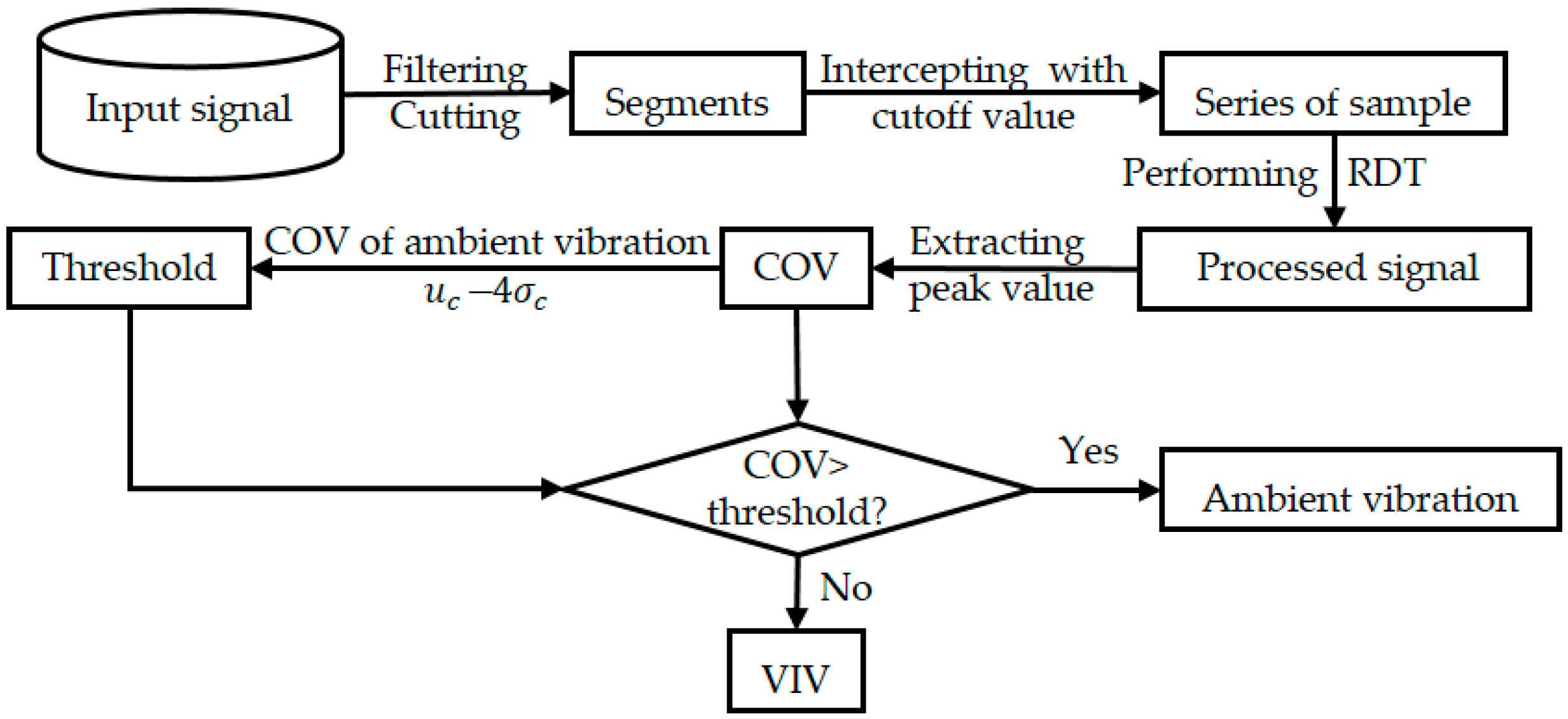
Figure 1 showed the flowchart of the proposed method for automatic identification of VIV from massive long-term monitoring data. In general, two steps are involved in this method. The first step is the establishment of a threshold of output, COV in this study, using random vibration data. In the second step, when the COV of new data fall below the threshold, the data will be identified as vortex-induced vibrations; otherwise it will be classified as random vibration.
In the first step, the raw acceleration data is processed with filtering to remove the undesired frequency components; a banded-pass filtering of 0.07–0.7 Hz is employed. The filtered data is processed by random decrement technique to obtain the random decrement signature from which the threshold is established.
2.2. Character of VIV and Random Vibration
A bridge at operation stage is usually subjected to ambient dynamic loadings, such as wind and traffic. When the dynamic loadings are random, the induced response will also be random, such as those caused by wind buffeting and passing vehicles. Wind buffeting is a kind of forced vibration caused by natural fluctuation of incoming wind. In some circumstances, the dynamic loading can be caused by periodic excitation such as vortex-shedding forces, and the induced response becomes periodic or even sinusoidal. Wind buffeting is usually not a serious concern due to its small amplitude at common wind velocity, while vortex-induced vibration can cause user discomfort and fatigue problems due to its large vibration amplitude up to 50 cm. The theoretical background of wind buffeting and vortex-induced vibration may be found in Simiu and Scanlan [1].
The majority of measured structural responses of a bridge at normal operation stage are random responses induced by wind buffeting and passing vehicles. Due to the broad-banded nature of excitation, random response is characterized by multimodal vibration, indicating a number of predominant frequency components in the power spectrum of random vibration. On the other hand, vortex-induced vibration is a kind of resonant vibration that is caused by the periodic shedding and its resulting sinusoidal forces. Therefore, VIV is characterized as single mode vibration for a specific wind velocity. Several distinct differences between random vibration and VIV are highlighted:
- (1)
- Random vibration is caused by the frequent random excitation, such as wind buffeting and passing vehicles. It is always occurring, regardless of the magnitude of wind velocity, while VIV occurs only at a specific wind velocity.
- (2)
- Random vibration is characterized by multiple mode responses, while VIV only has a single predominant frequency in the power spectrum.
Figure 2 showed the two typical segments from the health monitoring system of the Xihoumen Bridge, which corresponds to random vibration and VIV. It is obvious that the VIV signal is close to the harmonic signal, and is usually considerably larger than wind buffeting.
2.3. Random Decrement Technique
In this section, the background of RDT was briefly introduced. The random decrement technique is a time-domain method that uses the ensemble average of ambient data to approximate the free vibration responses when structures are exposed to linear, Gaussian white noise excitation. It was initially proposed by Cole in 1973 [28,29]. Later in 1982, Vandiver provided a strict mathematical proof for a single-degree-of-freedom system under the assumption of input to be a zero-mean, stationary, and Gaussian random process [27]. The technique can also be extended to multi-degrees-of-freedom systems naturally, and is identified as the multimode random decrement technique (MRDT) [30,31].
For a linear dynamical model, the forced vibration response, y(t), at a measurement point of a structure under any linear, Gaussian white noise excitation, f(t), can be expressed as:
where D(t) is free vibration response with an initial displacement of 1 and an initial velocity of 0; V(t) is free vibration response with an initial displacement of 0 and an initial velocity of 1; y(0) and (0) are initial displacement and velocity of the vibration system, respectively; h(t) is unit impulse response function of a viscously damped single-degree-of-freedom system; f(t) is dynamic loading; and ζ, ω, and ωd are modal damping ratio, natural frequency, and damped frequency, respectively.
As shown in Equation (1), the response y(t) in each time instant t can be decomposed as a linear superposition of three parts: The first two parts in the right hand side of Equation (1) represent the free vibration response due to initial displacement and initial velocity, and the third part is the forced vibration response due to dynamic loading, f(t). When f(t) follows a Gaussian white noise process, the responses, y(t), will also obey a Gaussian white noise process.
Figure 3 shows the overview of random decrement technique. By selecting an appropriate constant A to intercept a measured random vibration response signal, y(t), a series of sub-response process, y(t − ti), can be obtained as follow:
Since the f(t) is a zero-mean stationary Gaussian process, the starting point of time does not affect its random characteristics. By moving a series of time starting points ti of y(t − ti) to the origin of coordinate, a series of sample function, xi(t) (I = 1, 2, …, N), of random processes can be obtained:
Because f(t) and are zero-mean stationary Gaussian processes, the expectation of a sub- excitation process, E[f(t)], and the expectation of the sub-response process, E[], are zero. The mathematical expectation of xi(t) (I = 1, 2, …, N) is obtained as follows:
In practice, due to the limited measurement time and data, the average of x(t) is used to replace the mathematical expectation:
Therefore, a damped free vibration response with an initial displacement of A and an initial velocity of 0 is obtained.
2.4. Analysis of VIV Signal by RDT
The buffeting of the bridge is a kind of random vibration caused by turbulent flow, and the pulsating wind component in the atmosphere is the main contributing factor. Since pulsating wind is a stationary random excitation with a mean of zero, the response of the structure is also a stationary random response. It is therefore obvious that the buffeting response processed with RDT reduces to a kind of damped free-decaying response. In contrast, vortex-induced vibration is nearly a sinusoidal response with one dominant frequency, and VIV processed with RDT will become a harmonic response with nearly constant amplitude, as shown below.
The vortex-induced vibration of the bridge is a kind of wind-induced limiting vibration with both forced and self-excited properties. VIV events can be observed at a certain wind speed, and the measured vibration signal is close to the harmonic signal. Therefore, the harmonic response at a certain measurement point can be described as follows,
where Y is amplitude of the vibration; ω is circle frequency of the vibration, which is close to one of structural modal frequencies; θ is phase angle, which is a phase lag between force and structural response; η(t) is Gaussian white noise signal, which is a zero-mean stationary Gaussian process.
Likewise, the RDT is applied to vortex-induced vibration given by Equation (8). By selecting a constant A to intercept the signal, a series of segments can be obtained. The subsample function is given as follow:
Two subsamples of segments are taken as example for illustration, as follows
Similarly, ensemble average of yi(t) is given as follows:
It can be seen from the above equation that the VIV data processed with RDT becomes a harmonic signal.
2.5. Etablishment of Threshold-Discrimiating VIV and Random Vibration
As seen in Equations (7) and (11), there is a significant difference between the results of random vibration and VIV obtained with RDT. Specifically, the random vibration reduces to a kind of damped free vibration, while the VIV become a harmonic vibration. Figure 4 showed the obtained result of the acceleration data previously shown in Figure 2. It is verified that the result obtained from the random vibration is a damped free vibration, with the initial amplitude of 5 × 10⁻³ m/s2. As the length of the segment is limited, the number of the subsample that intercepted from the segment is limited, which makes the signal different from an ideal free vibration. By contrast, the amplitude of the VIV signal after the random decrement process changes little with time, remaining at about 5 × 10⁻² m/s2.
In order to distinguish the two kinds of responses given in Figure 4, the COV of peak values of the processed signals is used. First, the peak value of processed data is selected, and the COV of peak value is calculated for random vibration and for VIV. For random vibration signals, the COV of the random decrement signal will be significantly larger than that of VIV signal.
The calculation formula for COV is:
In order to determine the characteristic value of COV for random vibration, a large number of COV of the random vibration signal should be used. The mean value uc and the standard deviation σc are obtained from large data set of COV. In this paper, the Pauta criterion was considered when calculating the threshold for determining the VIV, the confidence interval was chosen as 99.99%:
When the COV is greater than the above threshold dc, the signal is determined as random vibration, and when the COV is less than the threshold, it is determined as a VIV. The main steps of the proposed method are summarized as follows:
- (1)
- Selecting the cutoff value A and the length of the output signal in the segment;
- (2)
- Performing the random decrement method to obtain the processed signal;
- (3)
- Extracting the peak value of the processed signal to obtain the COV of each signal segment;
- (4)
- Selecting a certain number of COV of the random vibration signal to obtain a threshold value;
- (5)
- Calculate the COV using steps (1)–(4) for a new data set. When the COV for the new data set is less than the threshold, it is identified as VIV.
3. Numerical Simulation
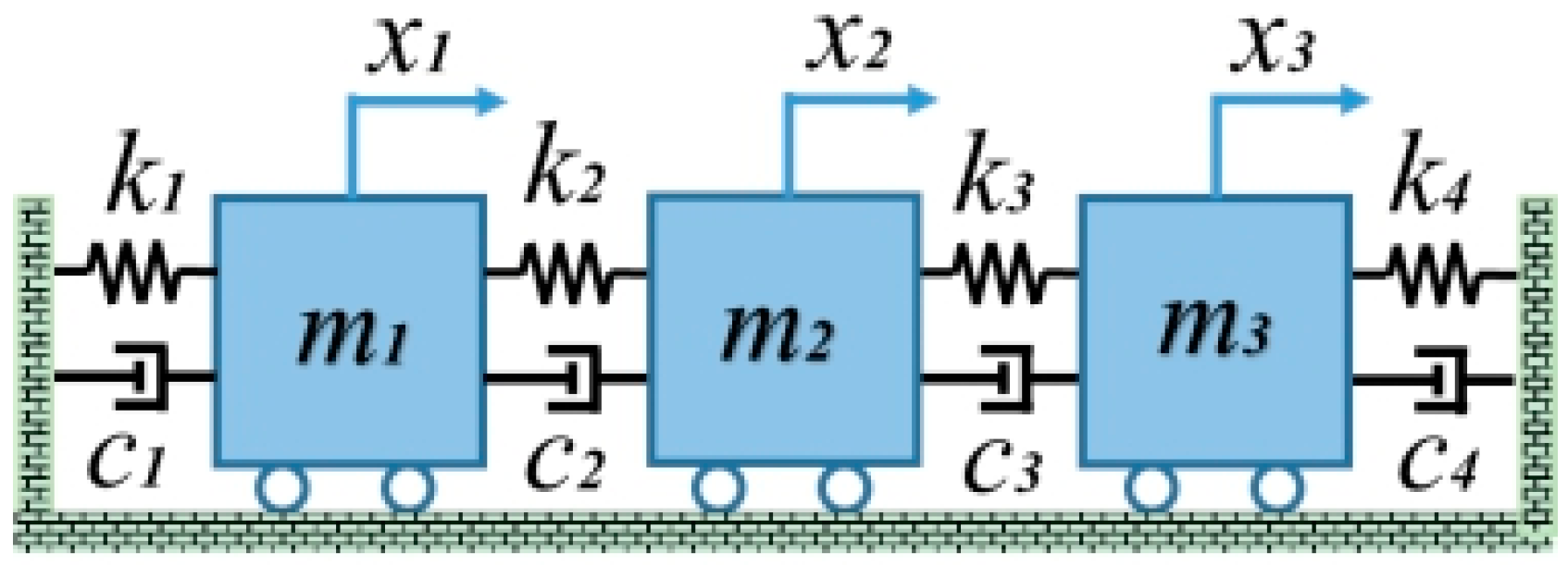
3.1. Description of a Three-DOF System
In order to verify the feasibility of the method proposed, a numerical example was carried out.Assuming a three-DOF mass-spring-damper system, as shown in Figure 5, where m1 = m2 = m3 = 400 kg, k1 = k4 = 20 kN/m, k2 = k3 = 25 kN/m, ci = 5ki. The natural frequencies of the above system were f1 = 0.874 Hz, f2 = 1.688 Hz, and f3 = 2.292 Hz. The damping ratios were ζ1 = 1.37%, ζ2 = 2.65%, and ζ3 = 3.60%. The frequencies of the second and third modes were relatively close.
3.2. VIV Identification Using RDT
In order to obtain the dynamic responses of the system, the Gaussian white noise excitation with zero mean was applied to the three masses firstly, and then the acceleration response of the three masses was calculated. The sampling frequency was 100 Hz and the sampling time was 1300 s. Next, the periodic vortex-induced force was simulated by harmonic excitation, F = (5~7 × 10⁻⁴)sin(2πf1t). The harmonic excitation was changed every 200 s to simulate the change of wind speed. Applying the harmonic force on m2 and considering noise at the same time. The sampling time was 600s. Finally, the Gaussian white noise excitation with zero mean value was applied to each mass unit again. The sampling time was 4100 s. The three segments were combined to simulate the whole process of vortex vibration, which was 6000 s totally. The load information of the three stagesis listed in Table 1 and the acceleration signal is shown in Figure 6.
In above figure, the signals of 0~1300 s and 1900~6000 s were the response signals caused by white noise excitation, and the signals from 1300 to 1900s were the response signals of m2 under the harmonic excitation with noise (0.03 SNR, signal-to-noise ratio). The overall data was divided into a series of segments, and the length of each segment has a length of 120 s. The parameter used in RDT was as follows: the interception A = 1.0 × σ, the length of RD is about 35 s (corresponding to 30 cycles). If the data length is too short, it is difficult to perform meaningful RDT; on the other hand, the false negative rate of detecting VIV will increase if the data length is too long.
After applying RDT for each segment, the COV of peak value of processed data were then calculated. The result was shown in Figure 7. Based on the calculated COV of peak in each segment of buffeting responses, and the threshold value was determined as dc = 0.1822. When the COV was smaller than the threshold value, the signal was regarded as VIV. The COV for the data during 1320~1900 s was significantly less than the threshold, thus they were identified as VIV. The identification results of VIV were shown in Table 2. It was shown that the vibration type was correctly identified except for the data during 1200–1320 s. It can be seen from the Table 2 that since 100 s buffeting signal and 20 s VIV signal were contained in 1200~1320 s, the identification result was random vibration. During 1800~1920 s, which contained 100 s VIV signal and 20 s buffeting signal, the identification result was VIV. The time interval can be appropriately adjusted, and the results of different time intervals can be combined to determine the VIV occurrence period.
Since the SNR can influence the identification result, the harmonic excitation with different SNR was applied to this three-DOF system, and the segment of 1320 to 1920 s was selected to further study. The SNR was changed from 0.001 to 0.03, and the simulation was repeated 1000 times at each SNR level. The number of segments identified as vortex-induced vibration was then divided by 1000, and named as the identification ratio. It can be seen in Figure 8 that the identification ratio was lower than 1 when the SNR was lower than 0.015. The power spectrum of two segments, with the SNR of 0.015 and 0.03 separately, were given in Figure 9. The ratio of the second to the first largest peak of the two spectrums were given as 0.27 and 0.05, thus the signal received from the harmonic excitation with SNR 0.015 is not VIV [24]. That means the SNR has little effect on this identification method. In summary, the simulation results demonstrated the feasibility of the method.
4. Application to the Xihoumen Bridge
4.1. Description of Bridge and SHM
The Xihoumen (XHM) Bridge is a two-span continuous suspension bridge with a 1650 m central main span and a 578 m side span, as shown in Figure 10. It carries asix-lane roadway by separated twin steel box girders, which are employed to improve the aerodynamic performance of the bridge against flutter. It is located in the sea area affected by typhoon, as shown in Figure 11. During the construction period, in September and October 2007, the bridge was attacked by typhoonsWipha and Rosa, respectively. Since it was opened to traffic in 2009, it has withstood many severe typhoons with wind velocity up to 50 m/s. However, at the normal wind velocity of 6~10 m/s, the VIV is easy to occur at the stiffening girder of the Xihoumen Bridge.
To measure the characteristics of the environmental loadings and the structural response of the bridge, a SHM system was implemented [32]. The environmental loadings monitored included the wind loads, vehicle loadings, the temperature, and humidity. The structural responses included displacement, acceleration, and strain of the bridge. There are various kinds of sensors, including ultrasonic anemometers, propeller anemometers, wind pressure transducers, GPS, and accelerometers. Those sensors were placed on the girder, towers, and some suspenders. In this paper, only the data from anemometers and accelerometers were used.
A propeller anemometer (PA) was installed on the top of the east side of each tower. The propeller anemometer can measure the wind speed and direction with a sampling frequency of 1Hz and a measuring range of 0~100 m/s. Six three-dimensional ultrasonic anemometers (UA), as shown in Figure 12, were installed on the bridge deck. Those anemometers can measure the three-dimensional wind velocity with a frequency of 32 Hz in the range of 0~65 m/s. Figure 13 showed the position of those two kinds of anemometers.
Thirty uniaxial accelerometers were installed on the stiffening girder and pylons of the bridge. Figure 14 illustrates the measurement locations for the accelerometers, where three accelerometers were positioned at each location. At position of AC1, AC2, AC3, and AC4, the three sensors in each position were arranged to obtain the vertical, lateral, and torsional acceleration responses. The positions of AC5, AC6, AC7, and AC8 were located at anchorages and piers, and they were used to measure the acceleration responses in vertical, lateral, and longitudinal directions. Three accelerometers were installed at the AC9, AC10, respectively. Two of them were used to measure the acceleration along the axis of the bridge and another one was used to measure the lateral accelerometers. Figure 15 showed two kinds of data acquisition instruments.
According to the description of bridge owners, the bridge experienced notable VIV by several dozen every year, which does cause discomfort to users. Based on the data recorded by the SHM of the Xihoumen Bridge in 2015, the proposed method was employed to identify the VIV events from massive long-term monitoring. The data in a whole year was up to 1 Terabyte. The acceleration data at the measuring stations of quarter and half span of the main span were used. The sampling frequency of the acceleration data was 50 Hz. The wind velocity measured at the two positions was also used, and the sampling frequency of wind was 32 Hz. The measured data in January, May, and August 2015 was used to identify the VIV events. According to modal analysis given below, it can be seen that the position of half span was the nodal point for the third, fifth, seventh, and ninth order modes, and the position of quarter span was the nodal point of the seventh mode. So according to the data of the half span, it was possible to identify the VIV, and the data of half span could be used to verify whether the identification result is correct. Since the measurement position of quarter span and half span were both the nodal point of the seventh order mode, the seventh mode cannot be identified by the peak method.
4.2. Structural Dynamic Characteristics
A finite element model of the Xihoumen Bridge was established to analyze the modal characteristic, and was shown in Figure 16. Beam element was adopted to simulate the main girder, towers, and piers; cable element was adopted to simulate the cable and suspenders; and mass element was adopted to simulate the ancillary facilities in the bridge. The anchorage point of the main cable and the tower bottom are both fixed with the foundation. At the position of the south tower, tower and girder are coupled in the lateral direction, vertical direction, and rotating around the axis, and only coupled in the lateral direction at the position of the north tower. The mode shapes for the first nine vertical-bending modes obtained from the finite element model were shown in Figure 17. The frequency characteristics of the vertical modes, identified from the acceleration responses of the bridge girder by peak-picking method are shown in Table 3 for comparison. A good agreement between analytical and experimental modal frequencies is observed.
4.3. Bridge Wind Field
As shown in Figure 11, the Xihoumen Bridge spans the narrow waterway between Cezi Island (North) and Jintang Island (South). According to its geographical location, the Xihoumen Bridge will not only encounter low velocity wind but also typhoons with much higher wind velocity. Therefore, the bridge encounters a large wind velocity range. As the largest suspension bridge in China at the time of 2019, it is very flexible and has multiple low natural frequencies, which are sensitive to dynamic wind action.
Figure 18 showed the wind rose diagram of the 10 min mean wind velocity at the quarter span of the bridge, measured in January, May, and August 2015. It can be seen that the 10 min mean wind velocity in three months is less than 20 m/s, and the wind direction distribution varies in different months. The northwest wind mainly occurs in winter and the southeast wind in summer. The wind direction distribution is the most dispersed in August. In the northwest direction, the wind direction varies greatly; for the southeast direction, most of the wind direction is almost perpendicular to the bridge. In general, the wind direction is likely to be perpendicular to the bridge, and this direction easily causes VIV. Additionally, the wind velocity changes in range, which may cause different modes of VIV in the bridge.
4.4. Identification of VIV
In order to obtain the threshold to identify VIV, the acceleration data without VIV were selected out by visual inspection ofthe data. These data included those on January 1 (wind velocity 2.5~14.5 m/s), January 17th (wind velocity 0.5~12 m/s), and May 10 (wind velocity 2.5~16 m/s), May 14 (wind velocity 0.5~12 m/s), and August 24 (wind velocity 2~15 m/s). For the data at the two measurement positions of quarter span and half span, the banded filtering process with the range of 0.07~0.7 Hz was performed at first. The data was then processed by the random decrement method, with the 10 min signal as input segment and the output segment length of 300 s. The threshold was calculated from the COV of peak values for each output segment. The thresholds of the two measuring points were shown in Table 4.
During the identification stage, all measured acceleration responses in January, May, and August are processed by random decrement method. If the COV for a segment is smaller than the threshold, it is considered as a VIV; otherwise it will be classified as wind buffeting. VIV is found on the first nine vertical modes of the XHM Bridge. By taking the data in January 4 as an example, as shown in Figure 19, it can be seen that VIV occurs at about 02:00 from the acceleration data at quarter span, while the data at half span does not indicate VIV. Another method based on artificial neural network (ANN) and the novelty detection technique is employed for automatic identification of VIV [24,33]. In this method, the power spectral density of the acceleration response was first used to construct a feature vector, and then a feature vector for random vibration was fed to ANN to train the model. In the test stage, any deviation from the expected output was classified as VIV. The results obtained from the novelty detection technique were shown in Figure 20. Again, the VIV is automatically detected from the acceleration response at quarter span.
The acceleration responses and the corresponding power spectrum at 02:00 were shown in Figure 21. In this figure, a single-mode vibration of the steady-state amplitude was observed at quarter span, and the predominant frequency is 0.1831 Hz, which corresponds to the third vertical bending mode of the girder. The vibration of half span behaves as random vibration. It can be seen from Figure 17 that the position of half span is close to the nodal point of the vibration mode, so the VIV of the third mode cannot be detected from the acceleration responses at the position of half span, and that is the reason why the power spectrum of the two points are different.
Another selected example of VIV observed on August 25 was shown in Figure 22. The identification result of both half span and quarter span indicates that the VIV occurred around 02:00, and the acceleration signals of half span and quarter span are likely at that period. As shown in Figure 22, the predominant frequency is 0.4322 Hz, which is associated with the eighth vertical mode of the girder.
Figure 23 showed the relationship between the 10 min mean wind velocity and the root mean square (RMS) of the displacement of VIV measured at the position of quarter span. It is obvious that the VIV happens mostly in the low wind velocity at 5 to 18 m/s. It can be seen that the wind velocity of each mode of VIV had a certain lock-in range, and the wind velocity range of adjacent modes partially overlapped. The overlap of lock-in velocity range for different modes suggests a hysteretic behavior or path dependency exists for VIV—whether the VIV develops from a lower velocity or from a higher velocity. The displacement of a high order mode, such as the seventh to ninth order, is apparently lower than others in this figure, which is partially caused by mode shape factor for different modes.
Figure 24 showed the relationship between the turbulence intensity for 10 min duration and the RMS of the VIV displacement for each mode. It can be seen that with increase of turbulence intensity the RMS amplitude of VIV generally decreased. However, for the sixth mode, significant VIV develop for a wide turbulence range, even for turbulence intensity as high as 13%. This observation suggests that the current section model tests for VIV may give unreliable results if modelling of turbulence is not respected.
5. Conclusions
In this study, an automatic identification method based on the random decrement technique was developed to detect VIV events from massive long-term continuous monitoring data. A simple COV-based threshold was demonstrated to successfully distinguish VIV from random vibration through numerical simulation of the three-DOF structure. The method was applied to automatically select out the VIV of the Xihoumen Bridge by using three-month monitoring data of acceleration, and the characteristics of VIV of the bridge was evaluated.
From the three-month monitoring data, a total number of 60 VIV events were successfully identified. The frequency range of VIV was between 0.1–0.5 Hz, which corresponds to the modal frequencies of the second to ninth vertical modes of stiffening girders. At wind velocity 5–18 m/s, different vertical modes were excited according to Stouhal number principle. Each mode had its own lock-in wind velocity; the Stouhal number was approximately 0.11. VIV happened most frequently for the third mode and sixth mode, which are symmetrical modes of vibration. A possible reason is that the symmetrical modes were less damped than the unsymmetrical modes. The maximum vibration amplitude of VIV at measurement locations was about 14 cm. Correlation with mean wind shows that the VIV happened mostly for the wind direction perpendicular to the bridge axis. VIV of some modes was observed for turbulence intensity up to 13%, and was less affected by turbulence intensity. The identified VIV events could be helpful for further understanding of VIV as well as its correlation with wind parameters. Evaluation of aerodynamic damping will also be carried out using the identified VIV data.
Author Contributions
Formal analysis, Z.H., and Y.L.; Methodology, X.H. and Q.W.; Motivation, Z.C.
Funding
The work was finically supported by NSFC (No. 51422806).
Conflicts of Interest
The authors declare no conflicts of interest.
References
- Simiu, E.; Scanlan, R.H. Wind Effects on Structures: Fundamentals and Applications to Design, 3rd ed.; John Wiley & Sons: New York, NY, USA, 1996. [Google Scholar]
- Sarpkaya, T. A critical review of the intrinsic nature of vortex-induced vibrations. J. Fluids Struct. 2004, 19, 389–447. [Google Scholar] [CrossRef]
- Wang, W.X.; Wang, X.Y.; Hua, X.G. Vibration control of vortex-induced vibrations of a bridge deck by a single-side pounding tuned mass damper. Eng. Struct. 2018, 173, 61–75. [Google Scholar] [CrossRef]
- Zhou, S.; Hua, X.G.; Chen, Z.Q.; Chen, W. Experimental investigation of correction factor for VIV amplitude of flexible bridges from an aeroelastic model and its 1:1 section model. Eng. Struct. 2017, 141, 263. [Google Scholar] [CrossRef]
- Weber, F.; Maslanka, M. Frequency and damping adaptation of a TMD with controlled MR damper. Smart Mater. Struct. 2012, 21, 55011–55027. [Google Scholar] [CrossRef]
- Frandsen, J.B. Simultaneous pressures and accelerations measured full-scale on the Great Belt East suspension bridge. J. Wind Eng. Ind. Aerodyn. 2001, 89, 95–129. [Google Scholar] [CrossRef]
- Allan, L.; Jens, H.W. A Two-Dimensional Discrete Vortex Method for Bridge Aerodynamics Applications. J. Wind Eng. Ind. Aerodyn. 1997, 67, 183–189. [Google Scholar]
- Fujino, Y.; Yoshida, Y. Wind-Induced Vibration and Control of Trans-Tokyo Bay Crossing Bridge. J. Struct. Eng. 2002, 128, 1012–1025. [Google Scholar] [CrossRef]
- Macdonald, J.H.G.; Irwin, P.A.; Fletcher, M.S. Vortex-induced vibrations of the Second Severn Crossing cable-stayed bridge—Full-scale and wind tunnel measurements. Proc. ICE Struct. Build. 2002, 152, 123–134. [Google Scholar] [CrossRef]
- Kim, H.K.; Kim, S.J.; Hwang, Y.C. Report of an Unexpected Vortex-Induced Vibration in an Actual Suspension Bridge. In Proceedings of the IABSE Symposium Report, IABSE Conference-Structural Engineering: Providing Solutions to Global Challenges, Geneva, Switzerland, 23–25 September 2015. [Google Scholar]
- Li, H.; Laima, S.J. Field monitoring and validation of vortex-induced vibrations of a long-span suspension bridge. J. Wind Eng. Ind. Aerodyn. 2014, 124, 54–67. [Google Scholar] [CrossRef]
- Cantero, D.; Oiseth, O.; Ronnquist, A. Indirect monitoring of vortex-induced vibration of suspension bridge hangers. Struct. Health Monit. 2017, 17, 837–849. [Google Scholar] [CrossRef]
- Kim, S.; Park, J.; Kim, H.K. Damping identification and serviceability assessment of a cable-stayed bridge based on operational monitoring data. J. Bridge Eng. 2017, 22, 04016123. [Google Scholar] [CrossRef]
- Brownjohn, J.M.W. Structural health monitoring of civil infrastructure. Philos. Trans. R. Soc. A 2007, 365, 589–622. [Google Scholar] [CrossRef]
- Memmolo, V.; Maio, L.; Boffa, N.D.; Monaco, E.; Ricci, F. Damage detection tomography based on guided waves in composite structures using a distributed sensor network. Optim. Eng. 2016, 55, 011007. [Google Scholar] [CrossRef]
- Fugate, M.L.; Sohn, H.; Farrar, C.R. Vibration-based damage detection using statistical process control. Mech. Syst. Signal Process. 2011, 15, 707. [Google Scholar] [CrossRef]
- Worden, K.; Farrar, C.R.; Manson, G.; Park, G. The fundamental axioms of structural health monitoring. Philos. Trans. R. Soc. A 2007, 463, 1639. [Google Scholar]
- Farrar, C.R.; Worden, K. Structural Health Monitoring: A Machine Learning Perspective; Wiley: New York, NY, USA, 2011. [Google Scholar]
- Song, G.B.; Wang, C.J.; Wang, B. Structural health monitoring of civil structures. Appl. Sci. 2017, 7, 789. [Google Scholar] [CrossRef]
- Yi, T.H.; Song, G.B.; Stiros, S.C. Distributed sensor networks for health monitoring of civil infrastructures. Shock. Vib. 2015, 2015, 271912. [Google Scholar] [CrossRef]
- Worden, K.; Manson, G.; Fieller, N.R.J. Damage detection using outlier analysis. J. Sound Vib. 2000, 229, 647. [Google Scholar] [CrossRef]
- Vitola, J.; Vejar, M.A.; Tibaduiza, D.A.; Pozo, F. Data-driven methodologies for structural damage detection based on machine learning applications. In Pattern Recognition: Analysis and Applications; Ramakrishnan, S., Ed.; Intechopen: Primorje-Gorski Kotar, Croatia, 2016. [Google Scholar]
- Rogers, T.J.; Worden, K.; Fuentes, R.; Dervillis, N.; Tygesen, U.T.; Cross, E.J. A Bayesian non-parametric clustering approach for semi-supervised structural health monitoring. Mech. Syst. Signal Process. 2019, 119, 100. [Google Scholar] [CrossRef]
- Li, S.W.; Laima, S.J.; Li, H. Cluster analysis of winds and wind-induced vibrations on a long-span bridge based on long-term field monitoring data. Eng. Struct. 2017, 138, 245–259. [Google Scholar] [CrossRef]
- Li, S.W.; Laima, S.J.; Li, H. Data-driven modeling of vortex-induced vibration of a long-span suspension bridge usingdecision tree learning and support vector regression. J. Wind. Eng. Ind. Aerod. 2018, 172, 196–211. [Google Scholar] [CrossRef]
- Huan, S.L.; McInnis, B.C.; Denman, E.D. Analysis of the random decrement method. Int. J. Syst. Sci. 1983, 14, 417–423. [Google Scholar] [CrossRef]
- Vandiver, J.K.; Dunwoody, A.B.; Campbell, R.B.; Cook, M.F. A Mathematical Basis for the Random Decrement Vibration Signature Analysis Technique. J. Mech. Des. 1982, 104, 307–313. [Google Scholar] [CrossRef]
- Cole, H.A. On-Line Failure Detection and Damping Measurement of Aerospace Structures by Random Decrement Signatures; NASA Cr-2205; Nat. Aeronautics and Space Administration: Washington, DC, USA, 1973.
- Cole, H.A. On the line analysis of random vibration. In Proceedings of the AIAA/ASME 9th Structures, Structural Dynamics and Materials Conference, Palm Springs, CA, USA, 1–3 April 1968. [Google Scholar]
- Tamura, Y.; Zhang, L.M.; Yoshida, A.; Nakata, S.; Itoh, T. Ambient vibration tests and modal identification of structures by FDD and 2DOF-RD technique. In Proceedings of the Structural Engineers World Congress, Yokohama, Japan, 9–12 October 2002. [Google Scholar]
- Wen, Q.; Hua, X.G.; Chen, Z.Q. AMD-Based Random Decrement Technique for Modal Identification of Structures with Close Modes. J. Aerosp. Eng. 2018, 31, 04018057. [Google Scholar] [CrossRef]
- Liu, Z.Q.; Li, N.; Guo, J. Design and implementation of structural monitoring systems for Xihoumen Bridge (II): Implementations. Eng. Sci. 2010, 12, 101–106. [Google Scholar]
- Hua, X.G.; Sun, R.F.; Wen, Q. Automatic detection of vortex-induced resonance events in bridges using novelty detection. J. Vib. Eng. 2018, 31, 948–956. (In Chinese) [Google Scholar]
Figure 1.
Flowchart of the proposed method (coefficient of variation-COV, Random decrement technique-RDT, Vortex-induced vibration-VIV).
Figure 1.
Flowchart of the proposed method (coefficient of variation-COV, Random decrement technique-RDT, Vortex-induced vibration-VIV).

Figure 2.
Comparison of the measured acceleration responses: (a) Random vibration; (b)VIV (Vortex-induced vibration-VIV).
Figure 2.
Comparison of the measured acceleration responses: (a) Random vibration; (b)VIV (Vortex-induced vibration-VIV).

Figure 3.
Overview of the random decrement technique (RDT).

Figure 4.
Random decrement signal of random vibration and VIV: (a) Signal of random vibration; (b) signal of VIV.
Figure 4.
Random decrement signal of random vibration and VIV: (a) Signal of random vibration; (b) signal of VIV.

Figure 5.
Three-degree-of-freedom (DOF) system consisting of spring and damper.

Figure 6.
Time history of acceleration response at m2.

Figure 7.
Coefficient of variation (COV) COV of every 30 cycles with interval of 100 cycles.

Figure 8.
The identification result with different signal-to-noise ratio (SNR).

Figure 9.
(a) The power spectrum with signal-to-noise ratio (SNR) of 0.015; (b) the power spectrum with signal-to-noise ratio (SNR) of 0.3.
Figure 9.
(a) The power spectrum with signal-to-noise ratio (SNR) of 0.015; (b) the power spectrum with signal-to-noise ratio (SNR) of 0.3.

Figure 10.
Elevation of XHM Bridge.

Figure 11.
Location of Xihoumen (XHM) Bridge.

Figure 12.
Anemometers in XHM Bridge: (a) Ultrasonic anemometers; (b) propeller anemometer.

Figure 13.
Location of anemometers.

Figure 14.
Location of accelerometers in bridge girder and pylon.

Figure 15.
Date logging system: (a) Acceleration signal conditioner; (b) data acquisition sub-station.
Figure 15.
Date logging system: (a) Acceleration signal conditioner; (b) data acquisition sub-station.

Figure 16.
Finite element model of XHM Bridge.

Figure 17.
Main vertical modes for stiffening girder of XHM Bridge: (a) mode 1; (b) mode 2; (c) mode 3; (d) mode 4; (e) mode 5; (f) mode 6; (g) mode 7; (h) mode 8; (i) mode 9.
Figure 17.
Main vertical modes for stiffening girder of XHM Bridge: (a) mode 1; (b) mode 2; (c) mode 3; (d) mode 4; (e) mode 5; (f) mode 6; (g) mode 7; (h) mode 8; (i) mode 9.

Figure 18.
Wind rose diagramof XHM Bridge in different months: (a) January; (b) May; (c) August.

Figure 19.
Acceleration responses and the identification results on January 4: (a) Acceleration at quarter span; (b) acceleration at half span; (c) COV and threshold at quarter span; (d) COV and threshold at half span.
Figure 19.
Acceleration responses and the identification results on January 4: (a) Acceleration at quarter span; (b) acceleration at half span; (c) COV and threshold at quarter span; (d) COV and threshold at half span.

Figure 20.
Novelty index obtained using artificial-neural-network (ANN)-based novelty detection: (a) Quarter span; (b) half span.
Figure 20.
Novelty index obtained using artificial-neural-network (ANN)-based novelty detection: (a) Quarter span; (b) half span.

Figure 21.
Selected acceleration response and its power spectral density (PSD) on 1 January: (a) Acceleration at quarter span; (b) PSD at quarter span; (c) acceleration at half span; (d) PSD at half span.
Figure 21.
Selected acceleration response and its power spectral density (PSD) on 1 January: (a) Acceleration at quarter span; (b) PSD at quarter span; (c) acceleration at half span; (d) PSD at half span.

Figure 22.
The random decrement signal and power spectrum of the eighth mode VIV on 25 May 2015: (a) Acceleration at quarter span; (b) COV and threshold at quarter span; (c) acceleration at half span; (d) COV and threshold at half span; (e) the identified VIV signal at quarter span; (f) the identified VIV signal at half span; (g) PSD of VIV data at quarter span; (h) PSD of VIV data at half span.

Figure 23.
Relationship between 10 min mean wind velocity and root mean squares (RMS) of displacement at quarter span.
Figure 23.
Relationship between 10 min mean wind velocity and root mean squares (RMS) of displacement at quarter span.

Figure 24.
Relationship between turbulence intensity and root mean squares (RMS) of displacement at quarter span.
Figure 24.
Relationship between turbulence intensity and root mean squares (RMS) of displacement at quarter span.


Table 1.
Load information of the three stages.
| Stage | Last Time | Sampling Frequency | Load | Load Position |
|---|---|---|---|---|
| 1 | 1300 s | 100 Hz | Gaussian white noise | m1, m2, and m3 |
| 2 | 600 s | 100 Hz | F = (5~7 × 10⁻⁴)sin(2πf1t)+ noise | m2 |
| 3 | 4100 s | 100 Hz | Gaussian white noise | m1, m2, and m3 |
Table 2.
Comparison of identification results with actual situation.
| Time | Actual Situation | Identification Results |
|---|---|---|
| 0~1200 s | R* | R |
| 1200~1320 s | R-V | R |
| 1320~1800 s | V* | V |
| 1800~1920 s | V-R | V |
| 1920~6000 s | R | R |
R—random vibration; V—VIV.
Table 3.
Comparison between analytical and identified modal frequencies of XHM Bridge.
| Mode Order | 1st | 2nd | 3rd | 4th | 5th | 6th | 7th | 8th | 9th |
|---|---|---|---|---|---|---|---|---|---|
| Simulation (Hz) | 0.101 | 0.133 | 0.184 | 0.229 | 0.274 | 0.324 | 0.375 | 0.428 | 0.482 |
| Measurement (Hz) | 0.098 | 0.134 | 0.183 | 0.232 | 0.275 | 0.324 | 0.378 | 0.433 | 0.494 |
| Deviation (%) | 2.08 | 0.75 | 0.54 | 1.31 | 0.36 | 0.00 | 0.8 | 1.17 | 2.49 |
Table 4.
COV threshold for automatic identification of Vortex-induced vibration (VIV).
| Measuring point position | Quarter span | Half span |
| Value of threshold | 0.0653 | 0.0245 |
© 2019 by the authors. Licensee MDPI, Basel, Switzerland. This article is an open access article distributed under the terms and conditions of the Creative Commons Attribution (CC BY) license (http://creativecommons.org/licenses/by/4.0/).
Share and Cite
MDPI and ACS Style
Huang, Z.; Li, Y.; Hua, X.; Chen, Z.; Wen, Q. Automatic Identification of Bridge Vortex-Induced Vibration Using Random Decrement Method. Appl. Sci. 2019, 9, 2049. https://doi.org/10.3390/app9102049
AMA Style
Huang Z, Li Y, Hua X, Chen Z, Wen Q. Automatic Identification of Bridge Vortex-Induced Vibration Using Random Decrement Method. Applied Sciences. 2019; 9(10):2049. https://doi.org/10.3390/app9102049
Chicago/Turabian StyleHuang, Zhiwen, Yanzhe Li, Xugang Hua, Zhengqing Chen, and Qing Wen. 2019. "Automatic Identification of Bridge Vortex-Induced Vibration Using Random Decrement Method" Applied Sciences 9, no. 10: 2049. https://doi.org/10.3390/app9102049
Note that from the first issue of 2016, this journal uses article numbers instead of page numbers. See further details here.