Fault Feature Extraction and Enhancement of Rolling Element Bearings Based on Maximum Correlated Kurtosis Deconvolution and Improved Empirical Wavelet Transform

Abstract

In order to extract and enhance the weak fault feature of rolling element bearings in strong noise conditions, the Empirical Wavelet Transform (EWT) is improved and a novel fault feature extraction and enhancement method is proposed by combining the Maximum Correlated Kurtosis Deconvolution (MCKD) and improved EWT method. At first, the MCKD method is conducted to de-noise the signal by eliminating the non-impact components. Then, the Fourier spectrum is segmented by local maxima or minima in the envelope of the amplitude spectrum with a pre-set threshold based on the noise level. By building up the wavelet filter banks based on the spectrum segmentation result, the signal is adaptively decomposed into several sub-signals. Finally, by choosing the most meaningful sub-signal with the maximum kurtosis, the fault feature can be extracted in the squared envelope spectrum and teager energy operator spectrum of the chosen component. Both simulations and experiments are performed to validate the effectiveness of the proposed method. It is shown that the spectrum segmentation result of improved EWT is more reasonable than the traditional EWT in strong noise conditions. Furthermore, compared with commonly used methods, such as the Fast Kurtogram (FK) and the Optimal Wavelet Packet Transform (OWPT) method, the proposed method is more effective in the fault feature extraction and enhancement of rolling element bearings.

1. Introduction

Rolling element bearings are extensively used in various industrial applications, such as aircrafts, marine vessels, coal mining machines, manufacturing, etc., and their failure is one of the most frequent reasons for machine breakdowns and accidents [1,2,3]. Consequently, the fault diagnosis of rolling element bearings is of great significance and has attracted increasing attention in recent years. Generally, a series of cyclic impacts are generated and the resonant frequencies of bearings and adjacent components are excited, triggering the modulation phenomenon in the incipient stage of bearing faults [4]. The collected vibration signal contains rich information of machines. Therefore, the vibration analysis is a preferred approach to diagnose bearing faults [5,6,7], and the fault characteristic frequency is often considered as the vital indicator of rolling element bearing faults [8]. However, noises inevitably exist and may inhibit the extraction of the fault feature [9]. Therefore, the extraction of the weak periodic feature, which can identify the fault type and the damage level at the same time, has gained a leading role in the fault diagnosis of rolling element bearings [10,11].

Traditional approaches are based on the time domain or frequency domain analysis. In order to perceive and analyze the weak fault in rolling element bearings signals, state-of-the-art technologies, including the Wavelet Transform (WT) [12,13,14] and Empirical Mode Decomposition (EMD) [15,16], are introduced to detect the early failure under noise interference. It is known that both WT and EMD attempt to decompose the processed signal into a series of distinct modes. By analyzing certain modes, the dominant or interesting features can be obtained and separated from other irrelevant modes. WT, including both Discrete Wavelet Transform (DWT) and Wavelet Packet Transform (WPT), is one of the most widely used methods for signal de-noising. The time and scale spectra information of the fault is always carried by its corresponding wavelet sub-band signal component. Therefore, it is able to understand the physical meaning of the fault detection process. However, the prescribed subdivision scheme and predetermined basis functions cannot adaptively process a signal based on the information contained in the signal [17,18]. Correspondingly, EMD, proposed by Huang et al. [19], is capable of decomposing a signal into a set of distinct modes adaptively. These modes represent natural oscillatory modes imbedded in the signal and behave as basis functions derived from the signal itself. However, the lack of mathematical theory often leads to mode mixing or over-estimation phenomenon [17,20].

In 2013, by explicitly building an adaptive wavelet filter bank to segment the spectrum adaptively, Gilles [17] proposed a novel signal decomposition method and named it Empirical Wavelet Transform (EWT). Combining advantages of both WT and EMD, the EWT can construct the wavelet basis in an adaptive way and decompose a signal according to the contained information. Therefore, EWT has attracted much attention and been used in a variety of applications, including medicine, biology [21,22], and machinery [23,24,25,26,27,28,29,30,31,32,33]. The traditional spectrum segmentation is achieved by detecting local maxima or minima of the spectrum. However, the amount of pseudo-maxima and pseudo-minima caused by the strong background noise always leads to an improper segmentation of the spectrum. In order to solve this problem, some modifications about the spectrum segmentation have been proposed [34,35]. Amezquita-Sanchez and Adeli [34] presented an adaptive multiple signal classification-empirical wavelet transform (MUSIC-EWT) methodology. Different from the traditional EWT, the MUSIC algorithm is used to estimate the frequencies contained in the signal and to build appropriate boundaries in the MUSIC-EWT. Comparatively, to ensure each mono-component is modulated by the fault characteristic frequency, Pan et al. [35] used the local minima as segmentation boundaries and then conducted the spectrum segmentation based on the scale space representation with a pre-determined scale parameter. Finally, satisfying modes can be obtained by merging similar mono-components together.

However, these modifications ignore the spectrum shape of rolling element bearing vibration signal in noise conditions and fail to get a reasonable segmentation result. In order to avoid the inaccurate identification of the internal modes caused by the heavy background noise, pre-treatment or post-treatment are combined with the EWT to enhance the feature extraction performance. Zi et al. [36] used the wavelet spatial neighboring coefficient de-noising with data-driven threshold to increase the signal to noise ratio (SNR) before EWT. The effectiveness of the proposed method has been validated by analyzing two experimental cases. By developing a feasible and efficient spectrum segmentation method, Yang et al. [37] also proposed an enhanced EWT and validated the effectiveness of this method by using the bearing and gearbox signals. In 2016, Lin et al. [38] utilized EWT to decompose the acoustic emission (AE) signals to extract the bearing fault feature by calculating the correlated kurtosis (CK) of the mono-components. However, a suitable time interval in the calculation of CK is difficult to pre-define and the performance of the proposed method is not good enough for engineering applications. Therefore, it can be included that although literatures report variant EWT technologies for rolling element bearings, the faults diagnosis in heavy noise condition is still a difficult task.

In order to diagnose faults of the rolling element bearings in strong noise condition, the EWT is improved by calculating the envelope of amplitude spectrum, and a new fault feature extraction method based on the combination of the Maximum Correlated Kurtosis Deconvolution (MCKD) and improved EWT is proposed in this paper. Already proven as an efficient tool for enhancing the periodic impulses in fault diagnosis of rolling element bearings and gearboxes [39,40,41,42,43,44,45,46,47,48,49,50,51], the MCKD is firstly used to de-noise the collected vibration signal. Then, the vibration signal is decomposed into a set of modes by the improved EWT, which performs segmentation based on the local maxima or minima of the amplitude spectrum envelope. Finally, by calculating the squared envelope spectrum, the fault feature can be extracted from the selected EWT mode.

The remainder of this paper is organized as follows. The basic processes of MCKD and EWT are introduced in Section 2. Then, the EWT is improved and the fault feature extraction method is proposed by the combination of the MCKD and improved EWT in Section 3. Section 4 presents the preliminary validation of MCKD-EWT using simulations. Additionally, comparisons with the EMD, EWT, and improved EWT are also performed in this section. In Section 5, the real vibration signals from the bearing test rig are utilized to further validate the effectiveness of the proposed method by comparing the proposed method with FK (Fast Kurtogram) and OWPT (Optimal Wavelet Packet Transform) methods. Conclusions are summarized in Section 6.

2. The Basic Theory

2.1. MCKD Algorithm

MCKD encourages the periodicity of the periodic impacts or impulse-like vibration behaviors by selecting a finite impulse response (FIR) filter to maximize the CK of the filtered signal [44]. For an arbitrary collected vibration signal $x\left(n\right)$, which is caused by the bearing fault impulses $y\left(n\right)$, a reverse FIR filter f is needed to obtain $y\left(n\right)$ from $x\left(n\right)$.

$$y\left(n\right)={\displaystyle \sum _{k=1}^{L}f\left(k\right)}\hspace{0.33em}x\left(n-k+1\right)$$

(1)

where $k=1,2\cdots ,n$, and L is the length of the filter f.

The MCKD is used to search a reverse FIR filter f by maximizing the CK of the impulses $y\left(n\right)$. The CK is defined as:

$$C{K}_M\left(T\right)=\frac{{\displaystyle \sum _{n=1}^N{\left({\displaystyle \prod _{m=0}^M{y}_{n-mT}}\right)}^2}}{{\left({\displaystyle \sum _{n=1}^N{y}_n^2}\right)}^{M+1}}$$

(2)

where T is the period of impulses and M is the shift number.

The optimization function of MCKD is expressed as:

$$\underset{f}{\max }C{K}_M\left(T\right)=\underset{f}{\max }\frac{{\displaystyle \sum _{n=1}^N{\left({\displaystyle \prod _{m=0}^M{y}_{n-mT}}\right)}^2}}{{\left({\displaystyle \sum _{n=1}^N{y}_n^2}\right)}^{M+1}}$$

(3)

Apparently, the optimization function is used to find the optimal filter coefficients corresponding to the maximum of $C{K}_M\left(T\right)$. Namely,

$$\frac{d}{d{f}_k}C{K}_M\left(T\right)=0,\left(k=1,2\cdots L\right)$$

(4)

By solving Equation (4), the filter coefficients are finally expressed as follows,

$$f=\frac{{‖y‖}^2}{2{‖\beta ‖}^2}{\left(X_0{X}_0^T\right)}^{-1}{\displaystyle \sum _{m=0}^M\left(X_{mT}{\alpha }_m\right)}$$

(5)

where

$$X_{mT}={\left[\begin{array}{ccccc}{x}_{1-mT}& x_{2-mT}& x_{3-mT}& \cdots & x_{N-mT}\\ 0& x_{1-mT}& x_{2-mT}& \cdots & x_{N-1-mT}\\ 0& 0& x_{1-mT}& \cdots & x_{N-2-mT}\\ ⋮& ⋮& ⋮& \ddots & ⋮\\ 0& 0& 0& \cdots & x_{N-L-mT+1}\end{array}\right]}_{L\times N}$$

(6)

$${\alpha }_m=\left[\begin{array}{c}{y}_{1-mT}^{-1}\left(y_1^2{y}_{1-T}^2\cdots y_{1-mT}^2\right)\\ y_{2-mT}^{-1}\left(y_2^2{y}_{2-T}^2\cdots y_{2-mT}^2\right)\\ ⋮\\ y_{N-mT}^{-1}\left(y_N^2{y}_{N-T}^2\cdots y_{N-mT}^2\right)\end{array}\right]$$

(7)

$$\beta =\left[\begin{array}{c}{y}_1{y}_{1-T}\cdots y_{1-mT}\\ y_2{y}_{2-T}\cdots y_{2-\mathrm{m}T}\\ ⋮\\ y_N{y}_{N-T}\cdots y_{N-mT}\end{array}\right]$$

(8)

Equation (5) is nonlinear and can be solved iteratively through the following procedures.

Step 1.

Set the period of deconvolution T, the number of shift M, and the maximum iteration number n;

Step 2.

Compute $X_0$, $X_0^T$, and $X_{mT}$ by using the acquired signal x;

Step 3.

Initiate the filter coefficients f with L samples; Generally, the initial filter coefficients equals ${\left[\begin{array}{cccc}0\hfill & 0\hfill & \cdots \hfill & \begin{array}{cccc}1\hfill & -1\hfill & 0\hfill & 0\hfill \end{array}\hfill \end{array}\right]}^T$ to prevent the MCKD algorithm from converging to the local solution. The difference is in the center.

Step 4.

Calculate the output signal by Equation (1);

Step 5.

Compute ${\alpha }_m$ and $\beta$ based on signal y;

Step 6.

Update the filter coefficient f by Equation (5);

Step 7.

Determine whether the difference between iterations ($\Delta C{K}_M\left(T\right)$) is less than the given threshold. If this criterion is satisfied or the iteration equals n, then terminate the iteration progress; otherwise, the process is reverted back to Step 4;

Step 8.

Once the optimal filter coefficients f is obtained, the final output signal can be calculated using Equation (1).

For simplification, the derivation is not given here. However, the detailed derivations can be referred to in a previous study [44].

2.2. Empirical Wavelet Transform

In order to address the mode mixing or over-estimation phenomenon of the EMD method, Gilles [17] proposed an adaptive method named the empirical wavelet transform (EWT) method. The key step of EWT is segmenting the Fourier spectrum of the collected signal. EWT divides the spectrum into several portions, and each portion corresponds to a mode centered at the specific frequency and compact support, such as AM-FM signal. Assuming that we want to segment the Fourier spectrum into N continuous segments, it needs to find (N − 1) the largest local maxima in the Fourier spectrum. In most cases, 0 and $\pi$ are always taken as two boundaries (the Fourier spectrum is normalized). For this set of maxima, we define that ${\omega }_n$ is the boundary between each segment, where ${\omega }_0=0$ and ${\omega }_N=\pi$. Each segment is shown as $A_n=\left[{\omega }_{n-1},{\omega }_n\right]$, then ${\cup }_{n=1}^N{A}_n=\left[0,\pi \right]$.

Centered on each ${\omega }_n$, we define a transition phase $T_n$, with width $2{\tau }_n$ and ${\tau }_n=\gamma {\omega }_n$; $\gamma$ is properly chosen to get a tight frame and is given in Equation (9).

$$\gamma <{\min }_n\left(\frac{{\omega }_{n+1}-{\omega }_n}{{\omega }_{n+1}+{\omega }_n}\right)$$

(9)

According to the boundaries defined by the segmentation of the Fourier spectrum, a series of empirical wavelets can be constructed as bandpass filters based on the idea of the construction of both Littlewood-Paley and Meyer’s wavelets [52]. For $\forall n>0$, the empirical scaling function and the empirical wavelet function are defined by the following Equations (10) and (11), respectively.

$${\widehat{\varphi }}_{\hspace{0.33em}n}\left(\omega \right)=\left\{\begin{array}{ll}1,\hfill & \left|\omega \right|\le {\omega }_n-{\tau }_n\hfill \\ \cos \left[\frac{\pi }{2}\beta \left(\frac{1}{2{\tau }_n}\left(\left|\omega \right|-{\omega }_n+{\tau }_n\right)\right)\right],\hfill & {\omega }_n-{\tau }_n\le \left|\omega \right|\le {\omega }_n+{\tau }_n\hfill \\ 0,\hfill & otherwise\hfill \end{array}\right.$$

(10)

$${\widehat{\psi }}_n\left(\omega \right)=\{\begin{array}{ll}1,\hfill & {\omega }_n+{\tau }_n\le \left|\omega \right|\le {\omega }_{n+1}-{\tau }_{n+1}\hfill \\ \cos \left[\frac{\pi }{2}\beta \left(\frac{1}{2{\tau }_{n+1}}\left(\left|\omega \right|-{\omega }_{n+1}+{\tau }_{n+1}\right)\right)\right],\hfill & {\omega }_{n+1}-{\tau }_{n+1}\le \left|\omega \right|\le {\omega }_{n+1}+{\tau }_{n+1}\hfill \\ \sin \left[\frac{\pi }{2}\beta \left(\frac{1}{2{\tau }_n}\left(\left|\omega \right|-{\omega }_n+{\tau }_n\right)\right)\right],\hfill & {\omega }_n-{\tau }_n\le \left|\omega \right|\le {\omega }_n+{\tau }_n\hfill \\ 0,\hfill & otherwise\hfill \end{array}$$

(11)

The function $\beta \left(x\right)=x^4(35-84x+70x^2-20x^3)$, which is the most commonly used [16]. Therefore, for $\forall n>0$, Equations (10) and (11) can be simplified as follows:

$${\widehat{\varphi }}_{\hspace{0.33em}n}\left(\omega \right)=\left\{\begin{array}{ll}1,\hfill & \left|\omega \right|\le \left(1-\gamma \right){\omega }_n\hfill \\ \cos \left[\frac{\pi }{2}\beta \left(\frac{1}{2\gamma {\omega }_n}\left(\left|\omega \right|-\left(1-\gamma \right){\omega }_n\right)\right)\right],\hfill & \left(1-\gamma \right){\omega }_n\le \left|\omega \right|\le \left(1+\gamma \right){\omega }_n\hfill \\ 0,\hfill & otherwise\hfill \end{array}\right.$$

(12)

$${\widehat{\psi }}_n\left(\omega \right)=\{\begin{array}{ll}1,\hfill & \left(1+\gamma \right){\omega }_n\le \left|\omega \right|\le \left(1-\gamma \right){\omega }_{n+1}\hfill \\ \cos \left[\frac{\pi }{2}\beta \left(\frac{1}{2\gamma {\omega }_{n+1}}\left(\left|\omega \right|-\left(1-\gamma \right){\omega }_{n+1}\right)\right)\right],\hfill & \left(1-\gamma \right){\omega }_{n+1}\le \left|\omega \right|\le \left(1+\gamma \right){\omega }_{n+1}\hfill \\ \sin \left[\frac{\pi }{2}\beta \left(\frac{1}{2{\tau }_n}\left(\left|\omega \right|-{\omega }_n+{\tau }_n\right)\right)\right],\hfill & \left(1-\gamma \right){\omega }_n\le \left|\omega \right|\le \left(1+\gamma \right){\omega }_n\hfill \\ 0,\hfill & otherwise\hfill \end{array}$$

(13)

The EWT is defined in a similar way as the classic wavelet transform. The detailed coefficients $W_f^{\epsilon }\left(n,t\right)$ are given by the inner products of the signal and the empirical wavelets, namely,

$$W_f^{\epsilon }\left(n,t\right)=〈f,{\psi }_n〉={\displaystyle \int f\left(\tau \right)}\hspace{0.33em}\overline{{\psi }_n\left(\tau -t\right)}\hspace{0.33em}d\tau =F^{-1}\left(\widehat{f}\left(\omega \right)\overline{{\widehat{\psi }}_n\left(\omega \right)}\right)$$

(14)

The approximation coefficients $W_f^{\epsilon }\left(0,t\right)$ are given by the inner products of the signal and the scaling function, namely,

$$W_f^{\epsilon }\left(0,t\right)=〈f,{\varphi }_{\hspace{0.33em}1}〉={\displaystyle \int f\left(\tau \right)}\hspace{0.33em}\overline{{\varphi }_{\hspace{0.33em}1}\left(\tau -t\right)}\hspace{0.33em}d\tau =F^{-1}\left(\widehat{f}\left(\omega \right)\overline{{\widehat{\varphi }}_{\hspace{0.33em}1}\left(\omega \right)}\right)$$

(15)

The reconstruction signal and the empirical modes are determined by the following

$$\begin{array}{ll}f\left(t\right)\hfill & =W_f^{\epsilon }\left(0,t\right)\ast {\varphi }_{\hspace{0.33em}1}\left(t\right)+{\displaystyle \sum _{n=1}^N{W}_f^{\epsilon }\left(n,t\right)}\ast {\psi }_n\left(t\right)\\ & =F^{-1}\left(\widehat{W_f^{\epsilon }}\left(0,\omega \right){\widehat{\varphi }}_{\hspace{0.33em}1}\left(\omega \right)+{\displaystyle \sum _{n=1}^N\widehat{W_f^{\epsilon }}\left(n,\omega \right)}\hspace{0.33em}{\widehat{\psi }}_n\left(\omega \right)\right)\hfill \end{array}$$

(16)

$$f_{j=0}\left(t\right)=W_f^{\epsilon }\left(0,t\right)\ast {\varphi }_{\hspace{0.33em}1}\left(t\right)$$

(17)

$$f_{j=k}\left(t\right)=W_f^{\epsilon }\left(k,t\right)\ast {\psi }_k\left(t\right)$$

(18)

where $\ast$ denotes the convolution operator.

3. Fault Feature Extraction and Enhancement of Rolling Element Bearing Based on MCKD-EWT

3.1. Improved Empirical Wavelet Transform

The EWT provides an adaptive decomposition of the signal by detecting local maxima or minima of the spectrum; a large number of pseudo-maxima and pseudo-minima caused by the strong background noise will lead to an improper spectrum segmentation. Some researchers [34,35] have proposed modifications about the spectrum segmentation of the EWT. However, these modifications ignore the spectrum shape and fail to get a good segmentation in −5 dB or higher noise conditions. In order to avoid the inaccurate identification of these modes caused by the heavy background noise, an improved EWT method is proposed in this paper. A more reliable segmentation methodology for the signal spectrum is introduced by calculating the envelope curve of the amplitude spectrum of the signal. We calculate the envelope curve at first, and then modify the envelope curve with a pre-set threshold according to the SNR value. Finally, we segment the signal spectrum based on the local extrema of the modified envelope curve. The detailed progress of improved EWT is listed as the following:

Step 1.

Conduct FFT and obtain the Fourier spectrum $X\left(\omega \right)$ of the signal $x\left(t\right)$.

Step 2.

Calculate the following threshold according to the method of literature [35].

$$\lambda =A_l+r\left(A_h-A_l\right)$$

(19)

$$r=C/SNR$$

(20)

where $\lambda$ denotes the pre-set threshold, $A_h$ and $A_l$ are, respectively, the maximum and minimum magnitudes of the spectrum and r is inversely proportional to the SNR. Herein, a constant C is used to control the level of threshold. The larger the value of C, the higher the level of threshold tends to be. In this paper, r is taken to be 0.1 based on the assumption that the SNR of signals is higher than 85 dB and C = 10. The steps are continued as follows:

Step 3.

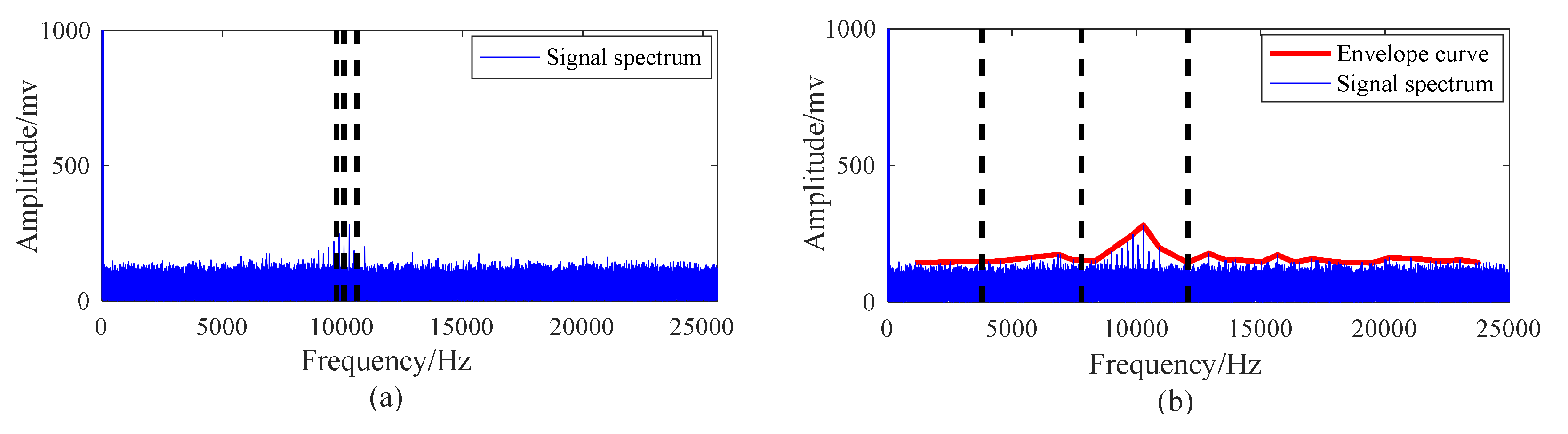
Calculate the envelope curve of the amplitude spectrum based on the local maxima and minima by linear interpolation method, then modify the envelope curve according to the threshold, and finally detect all the extras of the modified envelope curve. If the number of the local maxima points above the threshold is larger than the pre-defined number N of the components, then keep on calculating the envelope curve of the spectrum until the number of the local maxima points is equal or less than the pre-defined number N of the components. The number for the iteration process of the calculating envelope is always 5.

Step 4.

Obtain the segmentation boundaries. Detect all the local extrema points of the modified envelope curve, and then get the frequency bands of EWT modes by choosing the frequencies of local maxima points as the central frequencies of the modes. After that, locate the boundaries of each mode. Differing from the segmentation method, which uses the local minima points of the modified envelope curve as the boundaries of the EWT modes introduced in the literature, this method chooses the midpoints of the adjacent local minimum points as the segmentation boundaries. The detailed steps firstly calculate the midpoints of the adjacent local minimum points, and then sort them in ascending order, i.e., $\omega =\left[{\omega }_1,\cdots ,{\omega }_{n-1},{\omega }_n,\cdots ,{\omega }_N\right]$, which are used to segment the frequency spectrum. Finally, choose the ${\omega }_n$ between the adjacent local maximum points as the boundaries.

Step 5.

Segment the spectrum and choose the most meaningful component. Calculate the kurtosis value of each component and choose the component with the maximum kurtosis value to further detect the fault feature.

In the improved EWT method, the interference frequencies induced by the background noise can be restrained in the envelope curve of the signal spectrum. Therefore, the segmentation can be more accurate. Additionally, the numbers of the modes can be readily determined according to the detailed envelope shape of the actual signal. Consequently, the boundaries of these modes can be easily located according to the local extrema in the modified envelope curve.

3.2. Program of the Proposed Method

To extract the weak fault feature caused by the rolling element bearings in the heavy noise condition, a novel fault feature extraction and enhancement method is proposed by the combination of MCKD and improved EWT.

Suppose that the collected vibration is denoted by $x\left(t\right)$, which is composed of bearing fault components, rotor shaft fault components, background noise, etc. For the fault feature extraction of rolling element bearings, rotor shaft rotational frequency, harmonics, and any other interference frequencies should be eliminated. The proposed method solve such problems and the detailed program is listed as the following.

Step 1.

De-noise the signal by MCKD. De-noise the single accidental impact and non-impact components by implementing the MCKD to x(t). The key issue of the MCKD for a given bearing signal with faults is choosing these four parameters: the period of deconvolution T, the length of filter L, the termination number of iterations, and the number of shift M. The parameter T can be easily calculated based on the theoretical fault characteristic frequency, whereas L and M should be subjectively set without any reference. Whether the extracted fault signal is desired or not is severely influenced by the selected parameters. Therefore, selecting the optimal parameters is extremely important in MCKD. This method often chooses the termination number of iterations as a range from 20 to 30, the length of filter as a range from 100 to 300, the period of deconvolution T depending on the actual signal, and the shift number as a range from 2 to 5. Additionally, a method for setting parameters is recommended in a previous study [44].

Step 2.

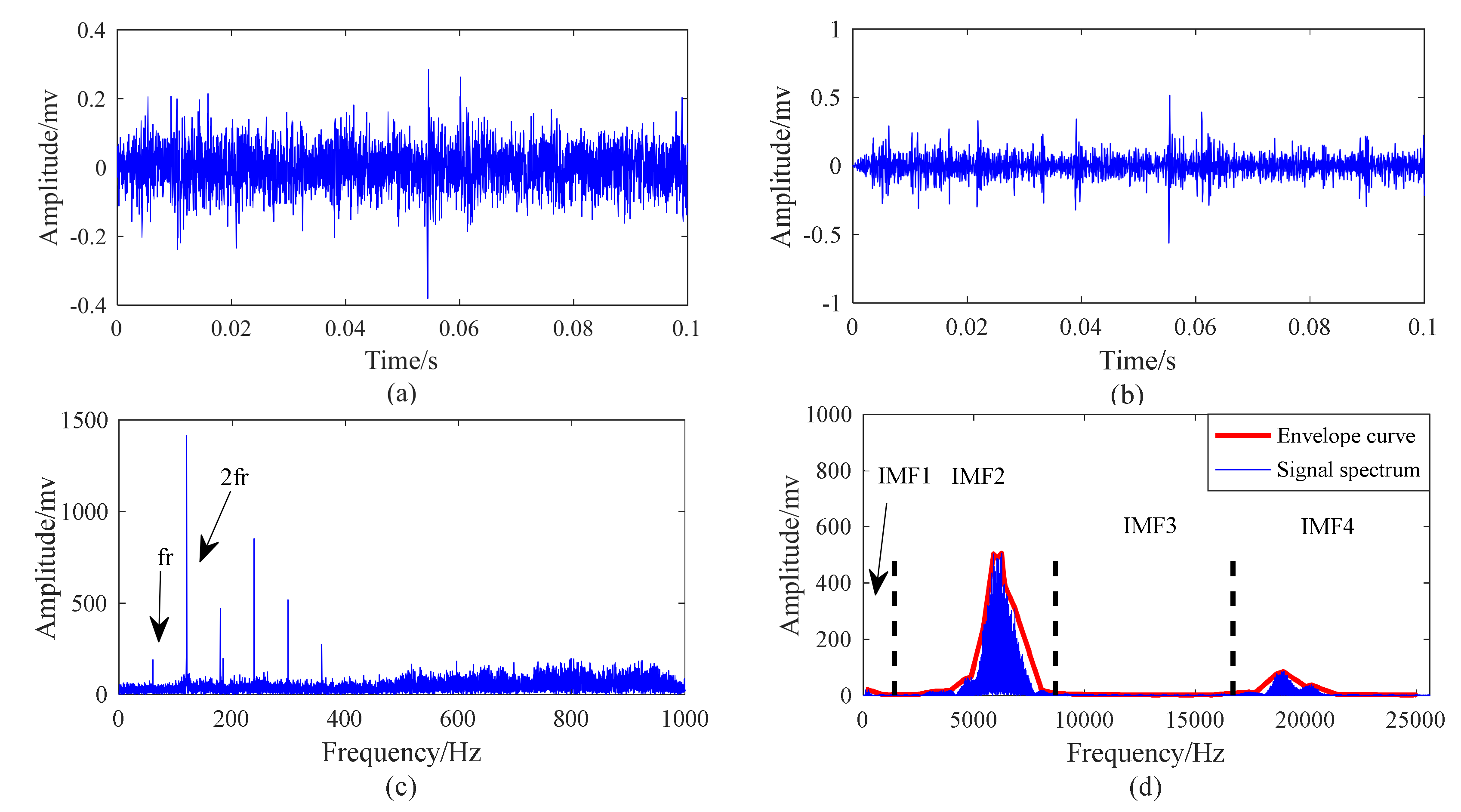
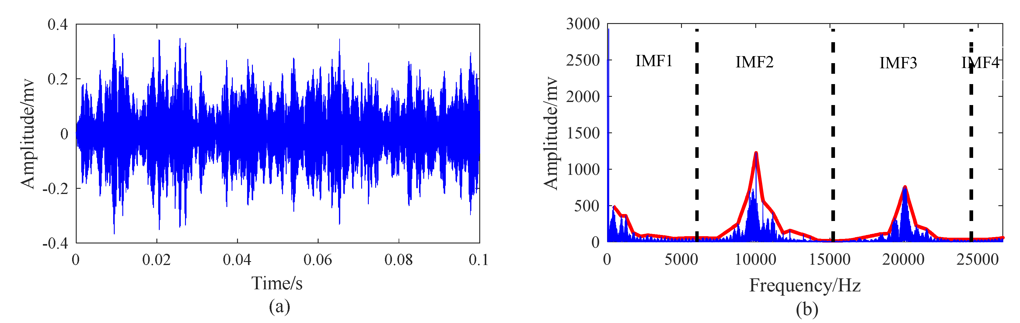
Spectrum segmentation. Calculate the envelope curve of the amplitude spectrum of the de-noising signal. Find the maxima and minima of the envelope curve and segment the spectrum on the modified envelope curve.

Step 3.

Signal decomposition. Design the wavelet filter banks based on the spectrum segmentation result and decompose the signal into several sub-signals.

Step 4.

IMF (Intrinsic Mode Function) selection. Calculate the kurtosis of each sub-signal and choose the best sub-signal with the maximum kurtosis.

Step 5.

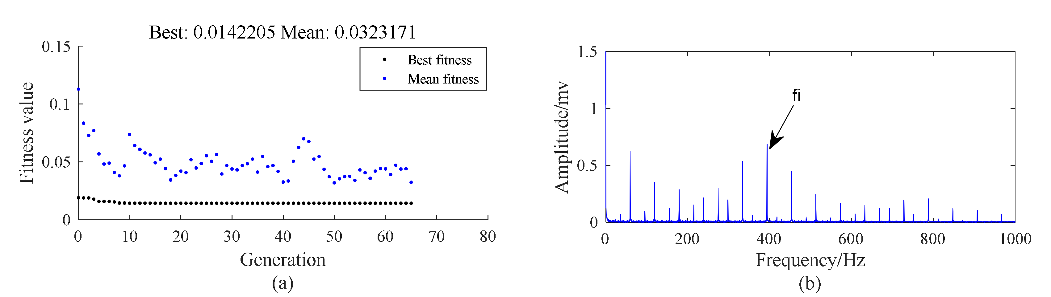
Feature extraction. Calculate the squared envelope spectrum and teager energy operator spectrum of the chosen mode. Analyze the fault characteristic frequency of the spectrum to determine the fault type and location of the fault.

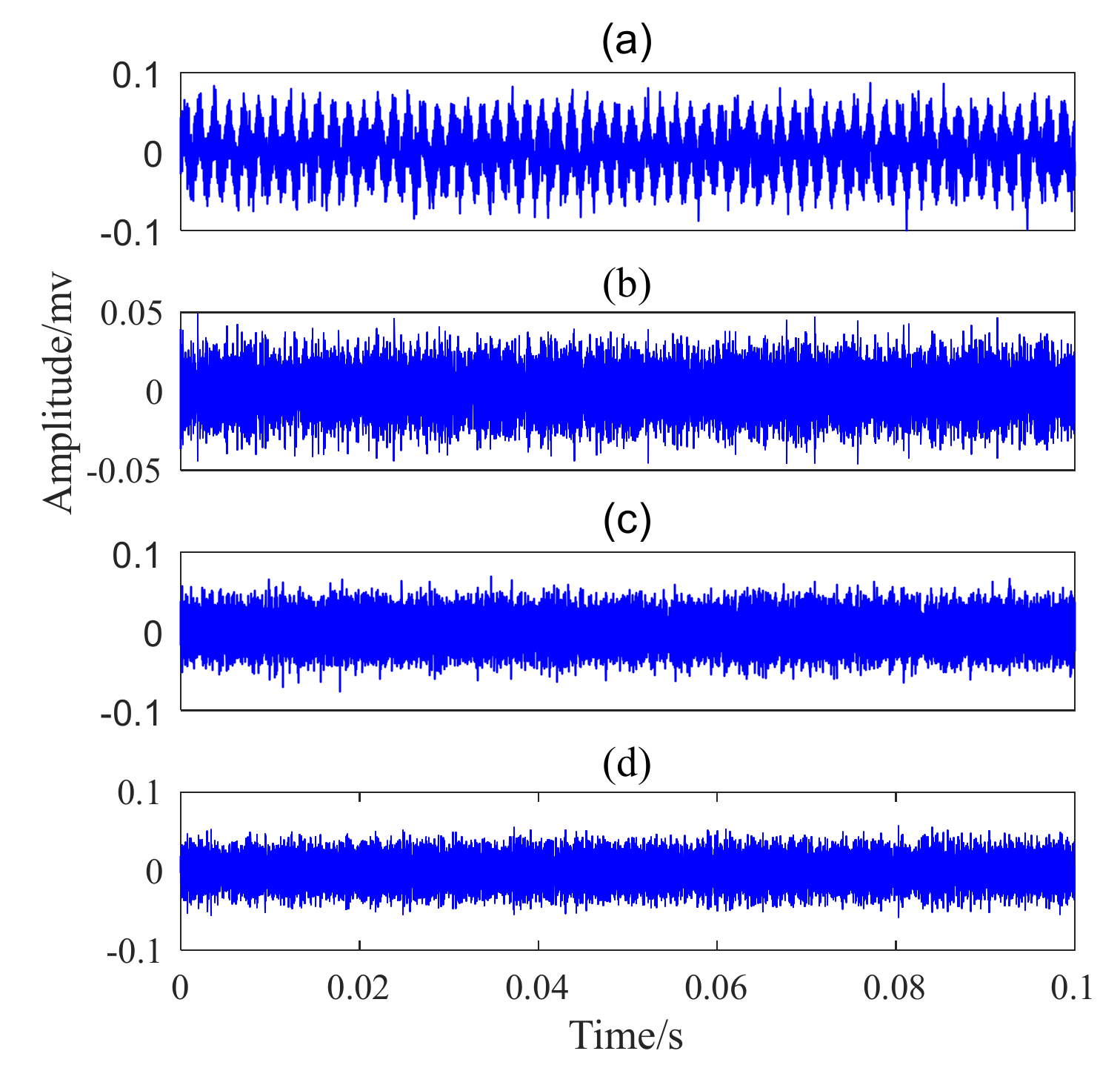
The program of the proposed method is simply illustrated in Figure 1.

4. Simulation

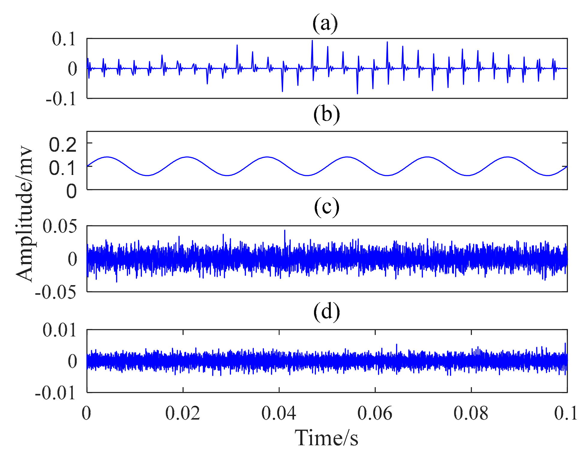
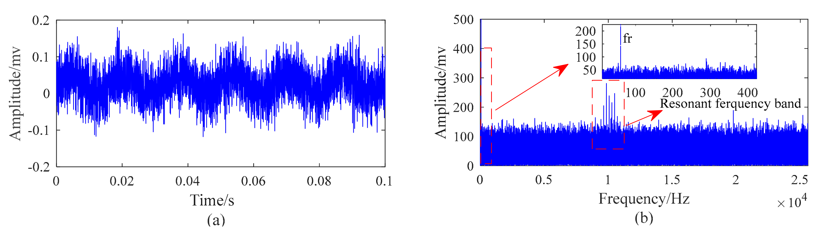
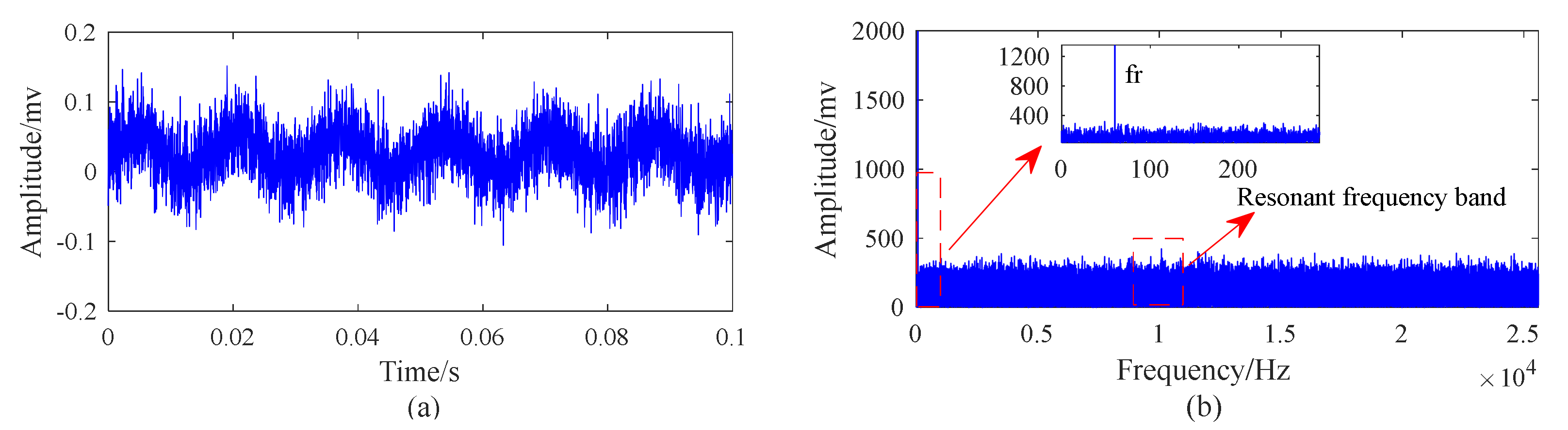
4.1. Model of the Collected Vibration

When a rolling element bearing fails, the rolling body will impact periodically when it touches the fault position [53,54,55,56]. Antoni and Randall [57] indicated that the vibration induced by a single fault in the rolling element bearing can be simulated as follows:

$$x\left(t_n\right)={\displaystyle \sum _{k=0}^{+\infty }{A}_k\exp \left(-\zeta 2\pi f_{\mathrm{n}}\left(t_n-T_k\right)\right)\cdot \sin \left(2\pi f_{\mathrm{n}}\left(t_n-T_k\right)+{\phi }_k\right)}$$

(21)

$$T_k=T_{k-1}+\Delta T_k,\hspace{1em}k=1,2,3,\dots$$

(22)

where $A_k$, determined by the rotational speed, load distribution, fault size, fault location, and other unknown factors in a complicated manner, denotes the amplitude of the kth transient response, $f_{\mathrm{n}}$ denotes the resonance frequency of the system, $\zeta$ denotes the relative damping ratio, ${\varphi }_{\hspace{0.33em}k}$ denotes the initial phase angle of the kth response, $T_k$ denotes the trigger time of the kth impulse, and $\Delta T_k$ denotes the interval time between the (k − 1)th and the kth impulses. It is proved that $\left\{T_k,k=1,2,3,\dots \right\}$ is an independent increment process because the rolling elements experience some random slippages, which depend on the rotational speed and load distribution in the actual operation programs, among other factors. If such random influence is neglected, the vibration is reduced to be periodical. Denoting $\Delta T$ as the average interval time of $\left\{\Delta T_k,k=1,2,3,\dots \right\}$, the slippage degree can be described by ${\sigma }_{\Delta T}$, the variance of $\left\{\Delta T_k,k=1,2,3,\dots \right\}$. Because $\Delta T_k$ is independently and identically distributed, the series of $\left\{\Delta T_k,k=1,2,3,\dots \right\}$ is modeled by white noise, the average value of which is $\Delta T$, and variance ${\sigma }_{\Delta T}$ equals the product of fluctuation and $\Delta T$.

$$\Delta T=\mathrm{E}\left\{\Delta T_k\right\}, k=1,2,3,\dots$$

(23)

$${\sigma }_{\Delta T}=fluctuation\times \Delta T$$

(24)

The simulation parameters are listed as follows: $A_k$ equals 1, $f_n$ equals 10 kHz, $\zeta$ equals 0.1, ${\varphi }_{\hspace{0.33em}k}$ equals 0, $\Delta T$ equals 2 ms, and the pre-amplified factor equals 80 dB. The sampling frequency is 51.2 kHz. The rotational frequency of the bearing is set to be 60 Hz. The impulse forces are cyclically produced and excite the impulse responses of the system. The force caused by fault is $\left(1+\sin \left(2\pi f_{\mathrm{r}}\mathrm{t}\right)\right)$ N. The vibration signal with the length of 512,000 samplings is collected. Moreover, 0.5% degree of random fluctuation of rotational frequency is introduced and trend term, white noise, and color noise are added to make the simulation closer to the physical condition.

The components of the simulation signal are shown as Equation (25) and Figure 2,

$$x\left(t\right)=x_1\left(t\right)+x_2\left(t\right)+x_3\left(t\right)+x_4\left(t\right)$$

(25)

where the impact signal induced by the bearing fault is $x_1\left(t\right)=x\left(t_n\right)$, the trend term is $x_2\left(t\right)=0.025+\sin (120\pi t)$, $x_3\left(t\right)$ is the white noise with 0.04 variance, and $x_4\left(t\right)$ is the color noise with 0.01 variance. The waveforms and spectrum of the simulation signal are shown in Figure 3.

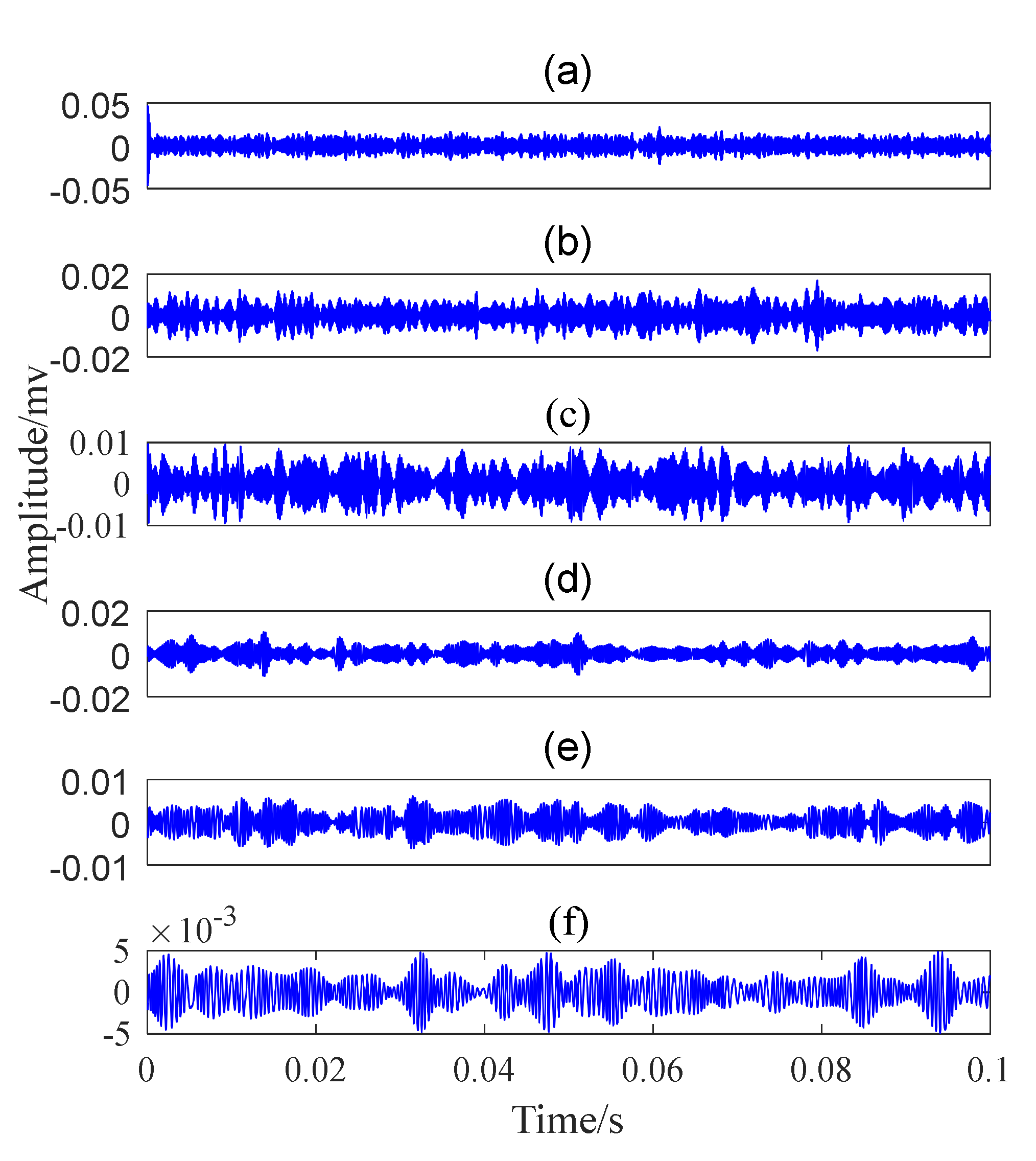
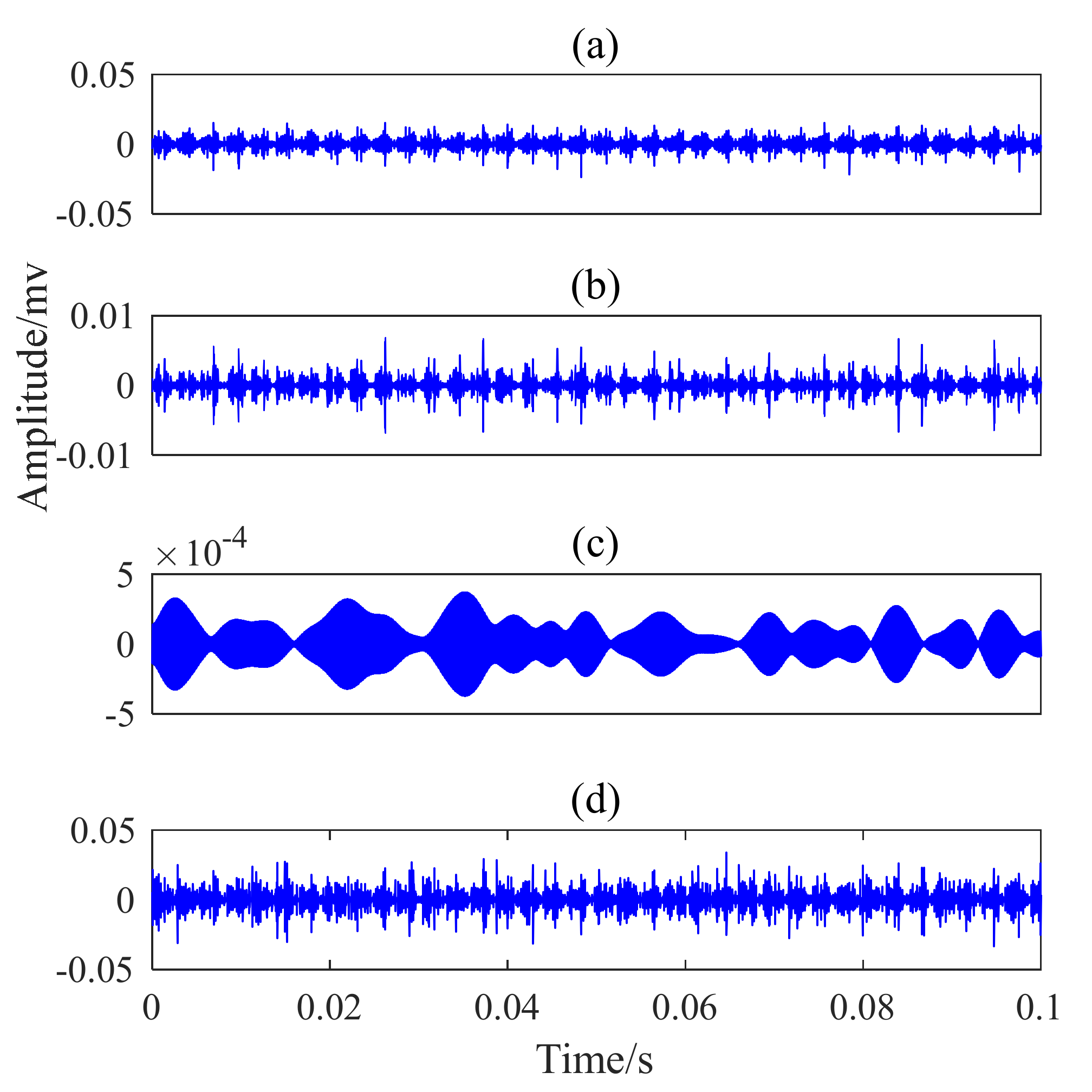
4.2. Comparison of Improved EWT, EWT, and EMD

To validate the efficiency of improved EWT, both EMD and EWT are conducted in this section. The results of EMD, EWT, and improved EWT are shown in Figure 4, Figure 5, Figure 6 and Figure 7. Nineteen modes are obtained by EMD and only the first six modes are shown in Figure 4. Compared with the original signal, the decomposed modes of EMD are mixed and overestimated. Comparatively, the segmentation results of EWT and improved EWT are illustrated in Figure 5, while the decompositions of both methods are shown in Figure 6 and Figure 7. It can be seen that no mode overestimation phenomenon can be noticed and the EWT is more consistent than the EMD. However, the segmentation boundaries are too dense in the local spectrum and the third mode is mixed. Differing from EMD and EWT, modes obtained by the improved EWT are consistent with the original signal.

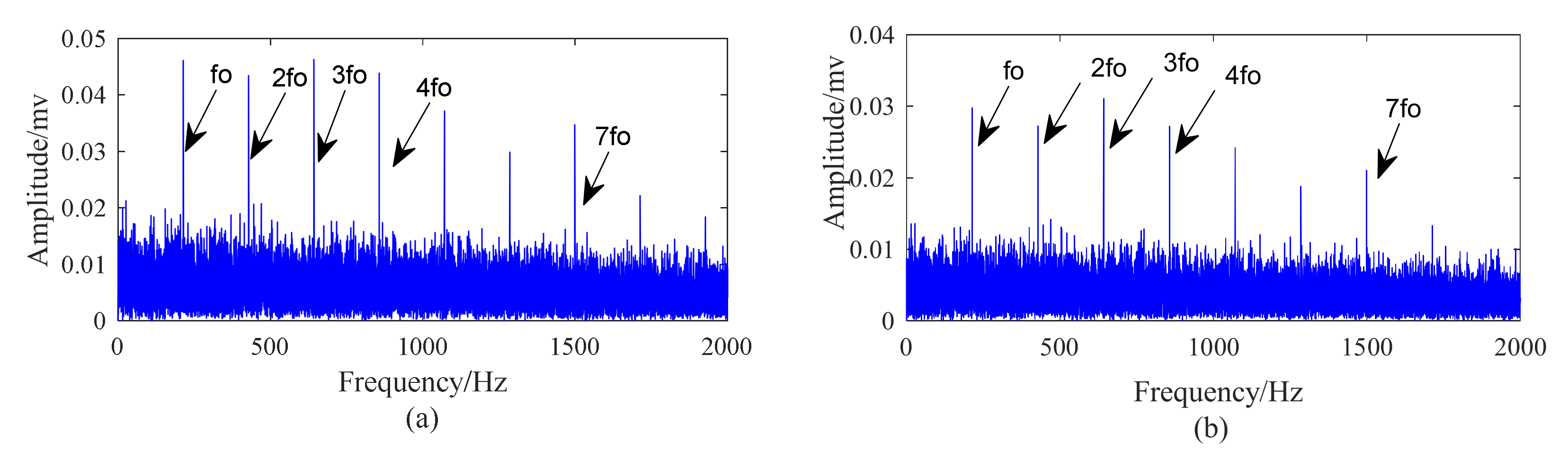
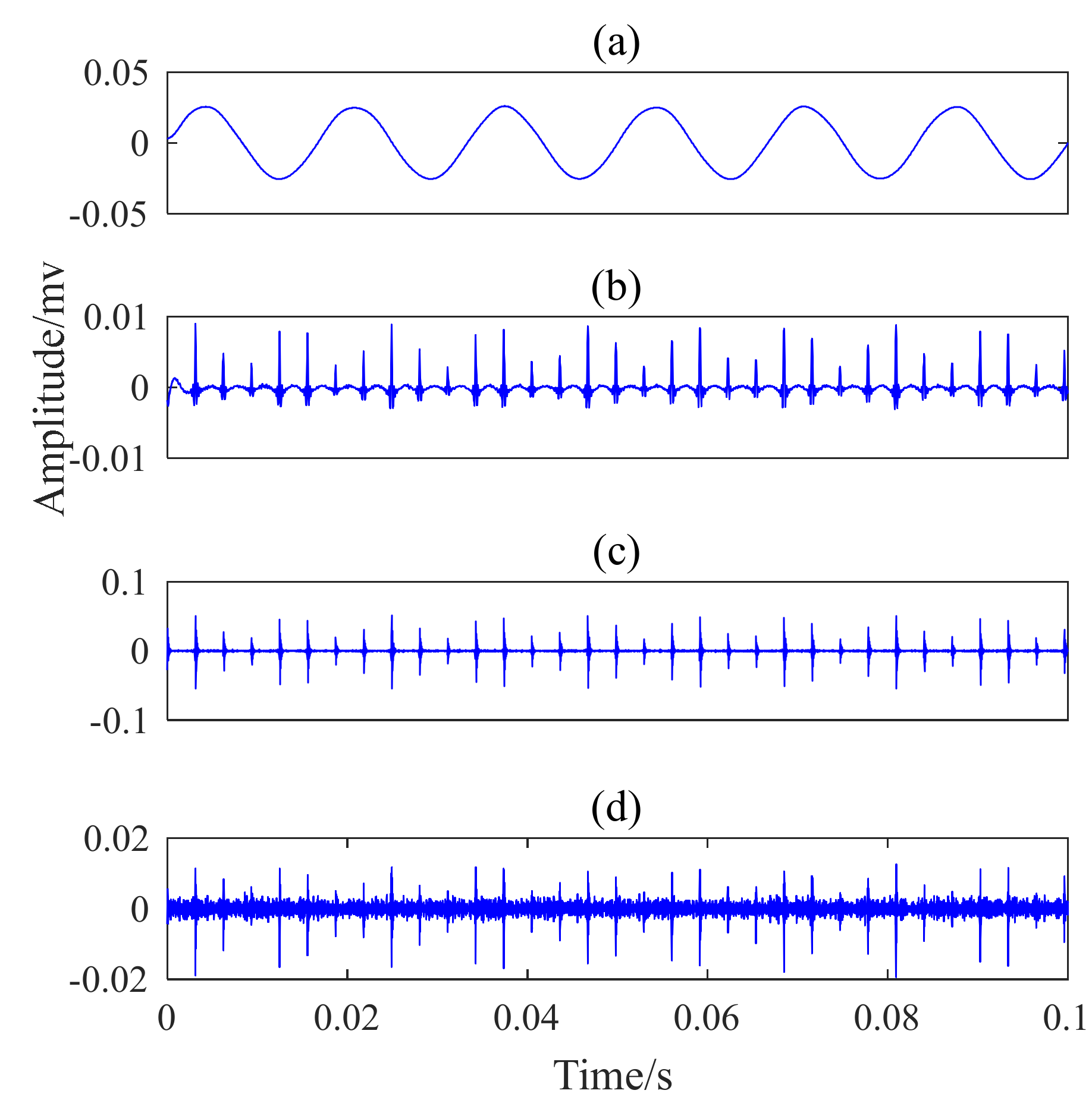
4.3. Outer Race Fault Simulation

In the simulation, the rotational frequency of the bearing system is 60 Hz, and the ratio of the ball pass frequency on the outer race (BPFO) to the rotational frequency is 3.57. The force caused by the fault is $\left(1+\sin \left(2\pi f_{\mathrm{r}}\mathrm{t}\right)\right)$ N. The resonant frequency of the system is 10 kHz and the relative damping ratio $\zeta$ is 0.1. Sampled at a frequency of 51.2 kHz and pre-amplified at 80 dB, the vibration signal with the length of 512,000 samplings is collected. Moreover, 0.5% degree of random fluctuation is introduced and −10 dB noise is added to make the simulation closer to the physical condition. The parameters of MCKD are set as follows: the period of deconvolution T is equal to 239, the length of filter L is equal to 90, the order of iteration is equal to 30, and the number of shift M is equal to 3, according to the method mentioned in Section 3.

The waveform and spectrum are shown in Figure 8. It can be seen that the impact responses are covered by noises and only rotational frequency can be found in the spectrum.

Figure 9a shows the signal obtained by MCKD. It can be seen that MCKD helps clarify the impacts of the signal. In Figure 9b, the Fourier spectrum of the pre-processed signal is segmented by EWT and the result can be seen in Figure 10.

The kurtosis values of these modes are, respectively, 3.0495, 3.216, 3.004, and 3.493. Figure 11 displays the squared envelope spectrum and teager energy operator spectrum of the selected signal mode 4. More than five dominant frequency spectrum lines located at the harmonics of the characteristic frequency (i.e., $f_o$, $2f_o$, $3f_o$, $4f_o$, and $5f_o$) can be recognized in Figure 11.

To validate the efficacy of the proposed method, both fast Kurtogram and OWPT are conducted on the simulated signal. What’s more, both the squared envelope spectrum and teager energy spectrum are used to show the detailed fault characteristic frequency. Figure 12 illustrated the fast Kurtogram (FK) and the squared envelope spectrum of the filtered signal. The FK result implies that the center frequency and the bandwidth of the optimal filter equal 19,200 Hz and 12,800 Hz, respectively. Compared to the original signal, the filtered signal cannot yet clearly characterize the fault feature of the simulated signal and no fault features can be noticed in Figure 12b.

The robust performance of the OWPT model is shown in Figure 13a. It can be seen that the mean fitness of the Genetic Algorithm (GA) training is 0.2835. The algorithm tends to be stable at 175th epoch and the fitness value reaches 0.178 at the 200th epoch. Figure 13b is the squared envelope spectrum obtained by OWPT. It implies that the architecture and parameters selected in the OWPT failed in the outer race fault feature extraction of the simulated signal.

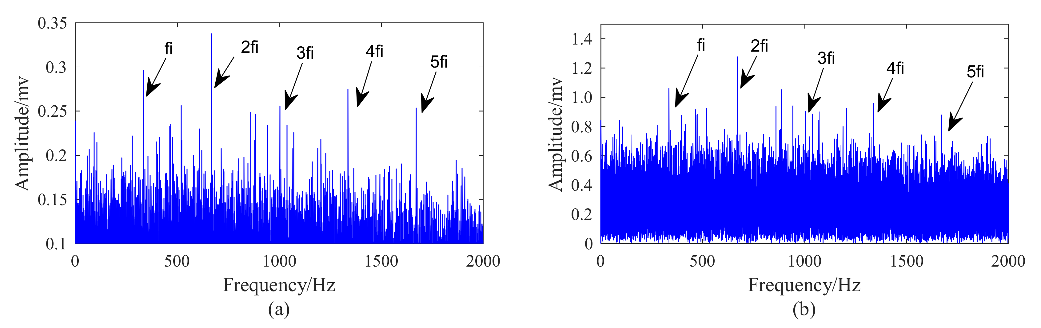
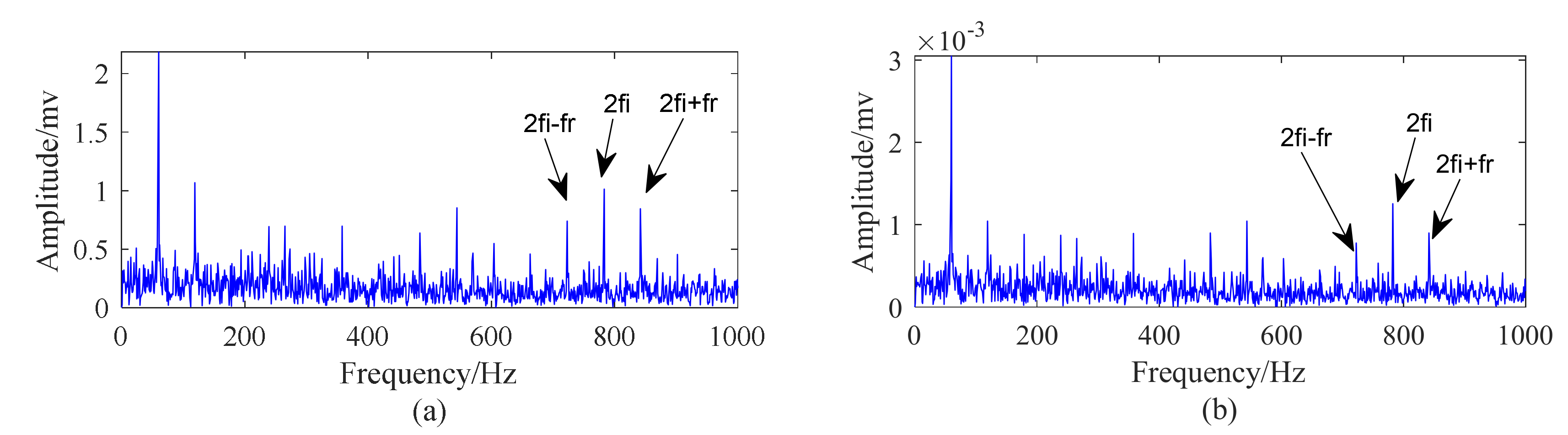
4.4. Inner Race Fault Simulation

In this section, cyclic impulse responses produced by an inner race fault are simulated based on the SDOF (Single Degree of Freedom) system, whose resonant frequency is 10 kHz, the relative damping ratio is 0.1, and the ball pass frequency on the inner race (BPFI) is 5.57 multiples of the rotational frequency. In this case, the force caused by the inner race fault is $\left(1+\sin \left(2\pi f_{\mathrm{r}}\mathrm{t}\right)\right)$ N, where $f_{\mathrm{r}}=60$ Hz denotes the rotational frequency. Sampled at the frequency of 51.2 kHz, the signal is pre-amplified at 80 dB and lasts 10 s. Moreover, 0.5% degree of random fluctuation is introduced and −10 dB noise is added to make the simulation closer to the physical condition. The parameters of MCKD are set as follows: the period of deconvolution T is equal to 153, the length of filter L is equal to 100, the order of iteration is equal to 20, and the number of shift M is equal to 3, according to the method mentioned in Section 3.

The waveforms and spectrum of the simulated signal are illustrated in Figure 14. It can be seen that the impact responses are covered by noises and only rotational frequency can be found in the spectrum.

Figure 15a shows the signal obtained by MCKD. It can be seen that MCKD helps clarify the impact of the signal. Figure 15b shows the spectrum segmentation by improved EWT and the decomposed modes are shown in Figure 16.

The kurtosis values of these modes are, respectively, 2.943, 3.029, 3.512, and 2.925. Figure 17 displays the squared envelope spectrum and teager energy operator spectrum of mode 3. It shows that the frequency 334.2 Hz and its harmonics (i.e., $f_i$, $2f_i$, $3f_i$, $4f_i$, and $5f_i$) can be recognized.

Figure 18 illustrates the FK and the squared envelope spectrum of the filtered inner race fault simulation signal. The Kurtogram implies that the center frequency and the bandwidth of the optimal filter equal 6400 Hz and 12,800 Hz, respectively. However, the squared envelope spectrum of the filtered signal is still dominated by the rotational frequency and noises and no fault features can be noticed.

The robust performance of the OWPT model is shown in Figure 19a. It can be seen that the mean fitness of the GA training is 0.2645. The algorithm tends to be stable at the 110th epoch and the fitness value reaches 0.148 at the 167th epoch. Figure 19b is the squared envelope spectrum obtained by OWPT. Obviously, it is similar to the outer race fault simulation case and no fault features can be involved in the squared envelope spectrum. It implies that the architecture and parameters selected in the OWPT are not effective for the inner race fault simulation signal with heavy noise.

5. Experiment

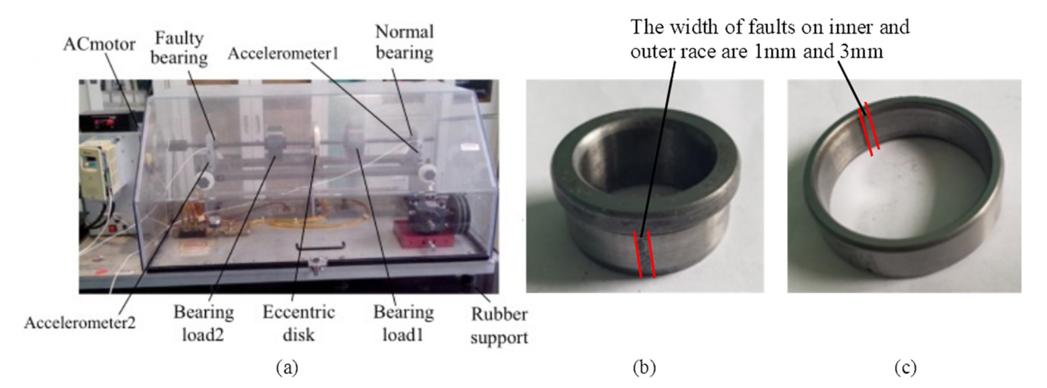
5.1. Experiment Apparatus

In this section, the effectiveness of the proposed method on weak fault diagnosis is validated by four experimental bearing cases, namely, inner race fault with circumferential width of 1 mm (which can be thought as small style fault like pitting), inner race fault with circumferential width of 3 mm (which can be thought as large style fault like stripping), outer race fault with circumferential width of 1 mm, and outer race fault with circumferential width of 3 mm on a 6204 E rolling element bearing. The experiment vehicle is shown in Figure 20.

The experiments are carried out on the machine fault simulator in the Machine Fault Diagnostics Laboratory of Tsinghua University. The rotor shaft with an eccentric disk in the middle of the shaft is supported by two bearings and is driven by an AC motor through a coupling. Two loads of 5 kg are used to load the bearing and the whole test-bed is supported by 8 rubbers on a desk. The fault bearing 6204 E, shown in Figure 20b,c, is located at the drive end of the rotor shaft. Similar to the simulation, the MCKD-EWT procedure is also applied to these experimental signals to validate the effectiveness of the proposed method.

5.2. Case 1: Outer Race Fault with Circumferential Width of 1 mm

The parameters of MCKD are set as follows: the period of deconvolution T is equal to 195, the length of filter L is equal to 90, the order of iteration is equal to 30, and the number of shift M is equal to 4, according to the method mentioned in Section 3.

From Figure 21a, it can be seen that the 1 mm outer race fault signal waveforms are buried in background noise. Figure 21b shows the signal is preprocessed by MCKD. It can be seen that MCKD helps clarify the impact of the signal. Figure 21c shows the spectrum of the outer race fault signal, and only rotational frequency and its harmonics can be found in the spectrum. In Figure 21d, the Fourier spectrum of the preprocessed signal is segmented by EWT and the result can be seen in Figure 22.

The kurtosis values of these modes are, respectively, 4.773, 9.035, 3.021, and 11.68. Figure 23 displays the squared envelope spectrum and teager energy operator spectrum of signal mode 4. In the squared envelope spectrum and teager energy operator spectrum, it can be seen that both methods successfully extract the outer race fault feature. The frequency 262 Hz and its harmonics (i.e., $f_o$, $2f_o$, and $3f_o$) are obvious in the strong background noise in Figure 23.

The FK is presented in Figure 24a. It implies that the center frequency and the bandwidth of the optimal filter equal 4800 Hz and 3200 Hz, respectively. The recommended frequency band of FK is $\left[\begin{array}{cc}3.2\hfill & 6.4\hfill \end{array}\right]$ kHz. Figure 24b illustrates the squared envelope spectrum of the filtered signal obtained by the recommended filter of FK. It can be seen that only rotational frequency and its harmonics can be found.

The robust performance of the OWPT model is shown in Figure 25a. It can be seen that the mean fitness of the GA training is 0.1331. The algorithm tends to be stable at the 5th epoch and the fitness value reaches 0.056 at the 57th epoch. Figure 25b is the squared envelope spectrum obtained by OWPT. Apparently, no fault feature can be noticed and it implies that the architecture and parameters selected in the OWPT are not effective and feasible for noisy signals.

5.3. Case 2: Outer Race Fault with Circumferential Width of 3 mm

The parameters of MCKD are set as follows: the period of deconvolution T is equal to 195, the length of filter L is equal to 90, the order of iteration is equal to 30, and the number of shift M is equal to 4.

From Figure 26a, it shows that the 3 mm outer race fault signal is buried in the background noise. Figure 26b shows the signal is preprocessed by MCKD. Figure 26c shows the spectrum of the outer race fault signal. In Figure 26d, the Fourier spectrum of the preprocessed signal is segmented by EWT and the result can be seen in Figure 27.

The kurtosis values of these modes are, respectively, 6.681, 8.715, 25.757, 9.928, and 19.664. Figure 28 displays the squared envelope spectrum and teager energy operator spectrum of signal mode 3. In the squared envelope spectrum and teager energy operator spectrum, it can be seen that both methods successfully extract the outer race fault feature. The frequency 262 Hz and its harmonics (i.e., $f_o$, $2f_o$, and $3f_o$) are obvious in the strong background noise in Figure 28.

The FK method is presented in Figure 29a. It implies that the center frequency and the bandwidth of the optimal filter equal 18,400 Hz and 1600 Hz, respectively. The recommended frequency band of FK is $\left[\begin{array}{cc}17.6\hfill & 19.2\hfill \end{array}\right]$ kHz. Figure 29b illustrates the squared envelope spectrum of the filtered signal obtained by the recommended filter of FK. It shows that both 262 Hz and its harmonics (i.e., $f_o$, $2f_o$, and $3f_o$) can be found.

The robust performance of the OWPT model is shown in Figure 30a. It can be seen that the mean fitness of the GA training is 0.1053. The algorithm tends to be stable at the 15th epoch and the fitness value reaches 0.0572 at the 72th epoch. Figure 30b is the squared envelope spectrum obtained by OWPT. The frequency 262 Hz and its harmonics (i.e., $f_o$, $2f_o$, and $3f_o$) can be noticed and it implies that OWPT is effective and feasible.

5.4. Case 3: Inner Race Fault with Circumferential Width of 1 mm

The parameters of MCKD are set as follows, the period of deconvolution T is equal to 131, the length of filter L is equal to 100, the order of iteration is equal to 30, and the number of shift M is equal to 3 according to the method mentioned in Section 3.

Figure 31 illustrates the original waveforms, spectrum, waveforms obtained by the MCKD, and the spectrum segmentation of the EWT. From Figure 31a,c, it can be seen that noise seriously disturbs the inner race fault diagnosis, and only rotational frequency and its harmonics can be found in the spectrum. Figure 31b shows the signal is preprocessed by MCKD. It can be seen that MCKD helps clarify the impact of the original signal. The Fourier spectrum of the preprocessed signal is segmented by EWT in Figure 31d and the result can be seen in Figure 32.

The kurtosis values of these modes are, respectively, 4.7467, 4.283, 18.447, and 39.525. Figure 33 displays the squared envelope spectrum and teager energy operator spectrum of the selected signal mode 4. In the squared envelope analysis and teager energy operator spectrum, it can be seen that both methods successfully extract the inner race fault feature. The frequency 392 Hz and its harmonics (i.e., $f_i$, $\left(f_i+f_r\right)$ and $2f_i$) are obvious.

The FK and corresponding squared envelope spectrum are presented in Figure 34. The recommended center frequency and bandwidth of the optimal filter are 22,000 Hz and 800 Hz, respectively. Namely, the recommended frequency band of FK is $\left[\begin{array}{cc}21.6\hfill & 22.4\hfill \end{array}\right]$ kHz. However, only rotational frequency and its harmonics can be found in the squared envelope spectrum.

The robust performance of the OWPT model is shown in Figure 35a. It can be seen that the mean fitness of the GA training is 0.0323. The algorithm tends to be stable at the 3rd epoch and the fitness value reaches 0.0142 at the 65th epoch. Figure 35b shows the squared envelope spectrum obtained by OWPT. It can be seen that several discrete spectral lines protrude at the frequencies of $f_r$, $n{f}_r$, $f_i$, and $f_i\pm f_r$.

5.5. Case 4: Inner Race Fault With Circumferential Width of 3 mm

The parameters of MCKD are set as follows: the period of deconvolution T is equal to 131, the length of filter L is equal to 100, the order of iteration is equal to 30, and the number of shift M is equal to 3.

Figure 36 illustrates the original waveforms, spectrum, waveforms obtained by the MCKD, and the spectrum segmentation of the EWT. From Figure 36a,c, it can be seen that noise seriously disturbs the inner race fault diagnosis, and only rotational frequency and its harmonics can be found in the spectrum. Figure 36b shows the signal preprocessed by MCKD. It can be seen that MCKD helps clarify the impact of the original signal. The Fourier spectrum of the preprocessed signal is segmented by EWT in Figure 36d and the result can be seen in Figure 37.

The kurtosis values of these modes are, respectively, 3.398, 3.323, 4.172, 3.658, and 3.725. Figure 38 displays the squared envelope spectrum and teager energy operator spectrum of the selected signal mode 3. In the squared envelope analysis and teager energy operator spectrum, it can be seen that both methods successfully extract the inner race fault feature. The $2f_i$ and $\left(2f_i\pm f_r\right)$ are obvious.

The FK and corresponding squared envelope spectrum are presented in Figure 39. The recommended center frequency and bandwidth of the optimal filter are 16,000 Hz and 2133 Hz, respectively. Namely, the recommended frequency band of FK is $\left[\begin{array}{cc}14.93\hfill & 17.06\hfill \end{array}\right]$ kHz. Both $f_i$ and its harmonics, $2f_i$, can be found in the squared envelope spectrum.

The robust performance of the OWPT model is shown in Figure 40a. It can be seen that the mean fitness of the GA training is 0.0226. The algorithm tends to be stable at the 3rd epoch and the fitness value reaches 0.0109 at the 51th epoch. Figure 30b is the squared envelope spectrum obtained by OWPT. We can find that several discrete spectral lines protrude at the frequencies of $f_i$, $f_i\pm f_r$, and $2f_i$.

Considering both outer and inner race fault cases, it is reasonable to conclude that the proposed method is more effective than the FK and OWPT methods in the weak fault feature extraction and enhancement of the rolling element bearing in strong noise conditions.

6. Conclusions

In order to diagnose the fault of the rolling element bearings in strong noise conditions, the spectrum segmentation strategy of EWT is improved and a novel fault feature extraction and enhancement method is proposed by the combination of MCKD and EWT. The non-impact components are de-noised by MCKD at first, and then the signal is decomposed by improved EWT. Both simulations and experiments are performed to validate the effectiveness of the proposed method by comparison with the FK and OWPT methods. Several useful conclusions are listed as follows.

Firstly, the improved EWT can adaptively segment the spectrum of the rolling element bearing in strong noise conditions. The modes number and frequency boundaries of each EWT mode can be easily determined, while the conventional EWT cannot segment the Fourier spectrum properly. In the proposed method, the influence induced by the single accidental impact and non-impact components is restrained after the de-noising process by the MCKD method, and then reasonable signal components can be obtained with the improved EWT method. This method can easily diagnose faults by choosing the best component with maximum kurtosis values and analyzing this signal component in the squared envelope spectrum and teager energy spectrum.

Secondly, compared with the FK and OPWT methods, the MCKD-EWT method is more effective in weak fault feature extraction and enhancement. When the fault is large enough, FK, OPWT, and MCKD-EWT methods can find the resonant frequency band and realize fault diagnosis. However, when the fault is small, FK and OPWT methods cannot find the resonant frequency band and result in a failure of fault diagnosis, while the MCKD-EWT method can realize the fault diagnosis by combining the advantages of MCKD and EWT. Therefore, the MCKD-EWT procedure is more powerful in engineering applications.

However, the detailed parameters of the MCKD-EWT procedure in this paper may not always be the best choice for the special bearing fault signal. When there is a large rotational speed fluctuation, the proposed method may be useless because the MCKD method needs to ensure the periodicity of the spacing of the pulses. The cost time of building the filters banks is too long, so it cannot be used in on-line fault diagnosis. Further investigation should be performed on choosing the optimal parameters of MCKD-EWT and finding an enhanced method for rotational speed fluctuations condition and finding a faster method.

References

1. Jiang, L.; Shi, T.; Xuan, J. Fault diagnosis of rolling bearings based on marginal fisher analysis. J. Vib. Control 2014, 20, 470–480. [Google Scholar] [CrossRef]
2. Randall, R.B. Vibration-Based Condition Monitoring: Industrial, Aerospace and Automotive Applications; John Wiley & Sons: Hoboken, NJ, USA, 2011. [Google Scholar]
3. Randall, R.B.; Antoni, J. Rolling element bearing diagnostics—A tutorial. Mech. Syst. Signal Proc. 2011, 25, 485–520. [Google Scholar] [CrossRef]
4. Lei, Y.; Lin, J.; He, Z.; Zi, Y. Application of an improved kurtogram method for fault diagnosis of rolling element bearings. Mech. Syst. Signal Process. 2011, 25, 1738–1749. [Google Scholar] [CrossRef]
5. Ou, L.; Yu, D.; Yang, H. A new rolling bearing fault diagnosis method based on GFT impulse component extraction. Mech. Syst. Signal Process. 2016, 81, 162–182. [Google Scholar] [CrossRef]
6. Li, Y.; Xu, M.; Wang, R.; Huang, W. A fault diagnosis scheme for rolling bearing based on local mean decomposition and improved multiscale fuzzy entropy. J. Sound Vib. 2016, 360, 277–299. [Google Scholar] [CrossRef]
7. Janjarasjitt, S.; Ocak, H.; Loparo, K.A. Bearing condition diagnosis and prognosis using applied nonlinear dynamical analysis of machine vibration signal. J. Sound Vib. 2008, 317, 112–126. [Google Scholar] [CrossRef]
8. Wang, D.; Peter, W.T.; Tsui, K.L. An enhanced Kurtogram method for fault diagnosis of rolling element bearings. Mech. Syst. Signal Process. 2013, 35, 176–199. [Google Scholar] [CrossRef]
9. Wang, Y.; He, Z.; Zi, Y. Enhancement of signal denoising and multiple fault signatures detecting in rotating machinery using dual-tree complex wavelet transform. Mech. Syst. Signal Process. 2010, 24, 119–137. [Google Scholar] [CrossRef]
10. Zhang, H.; Chen, X.; Du, Z.; Yan, R. Kurtosis based weighted sparse model with convex optimization technique for bearing fault diagnosis. Mech. Syst. Signal Process. 2016, 80, 349–376. [Google Scholar] [CrossRef]
11. Cui, L.; Wang, X.; Wang, H.; Wu, N. Improved fault size estimation method for rolling element bearings based on concatenation dictionary. IEEE Access 2019, 7, 22710–22718. [Google Scholar] [CrossRef]
12. Jayaswal, P.; Wadhwani, A.K. Application of artificial neural networks, fuzzy logic and wavelet transform in fault diagnosis via vibration signal analysis: A review. Aust. J. Mech. Eng. 2009, 7, 157–171. [Google Scholar] [CrossRef]
13. He, W.; Zi, Y.; Chen, B.; Wu, F.; He, Z. Automatic fault feature extraction of mechanical anomaly on induction motor bearing using ensemble super-wavelet transform. Mech. Syst. Signal Process. 2015, 54, 457–480. [Google Scholar] [CrossRef]
14. Liu, T.; Zhang, W.; Yan, S. A novel image enhancement algorithm based on stationary wavelet transform for infrared thermography to the de-bonding defect in solid rocket motors. Mech. Syst. Signal Process. 2015, 62, 366–380. [Google Scholar] [CrossRef]
15. Yu, D.; Cheng, J.; Yang, Y. Application of EMD method and Hilbert spectrum to the fault diagnosis of roller bearings. Mech. Syst. Signal Process. 2005, 19, 259–270. [Google Scholar] [CrossRef]
16. Feng, Z.; Zuo, M.J.; Hao, R.; Chu, F.; Lee, J. Ensemble empirical mode decomposition-based Teager energy spectrum for bearing fault diagnosis. J. Vib. Acoust. 2013, 135, 031013. [Google Scholar] [CrossRef]
17. Gilles, J. Empirical wavelet transform. IEEE Trans. Signal Process. 2013, 61, 3999–4010. [Google Scholar] [CrossRef]
18. Gilles, J.; Tran, G.; Osher, S. 2D empirical transforms. Wavelets, ridgelets, and curvelets revisited. SIAM J. Imaging Sci. 2014, 7, 157–186. [Google Scholar] [CrossRef]
19. Huang, N.E.; Shen, Z.; Long, S.R.; Wu, M.C.; Shih, H.H.; Zheng, Q.; Liu, H.H. The empirical mode decomposition and the Hilbert spectrum for nonlinear and non-stationary time series analysis. Proc. R. Soc. Math. Phys. Eng. Sci. 1998, 454, 903–995. [Google Scholar] [CrossRef]
20. Lei, Y.; Lin, J.; He, Z.; Zuo, M.J. A review on empirical mode decomposition in fault diagnosis of rotating machinery. Mech. Syst. Signal Process. 2013, 35, 108–126. [Google Scholar] [CrossRef]
21. Maheshwari, S.; Pachori, R.B.; Acharya, U.R. Automated diagnosis of glaucoma using empirical wavelet transform and correntropy features extracted from fundus images. IEEE J. Biomed. Health Inform. 2017, 21, 803–813. [Google Scholar] [CrossRef]
22. Bhattacharyya, A.; Pachori, R.B. A multivariate approach for patient-specific EEG seizure detection using empirical wavelet transform. IEEE Trans. Biomed. Eng. 2017, 64, 2003–2015. [Google Scholar] [CrossRef]
23. Hu, Y.; Li, F.; Li, H.; Liu, C. An enhanced empirical wavelet transform for noisy and non-stationary signal processing. Dig. Signal Process. 2017, 60, 220–229. [Google Scholar] [CrossRef]
24. Mao, J.; Li, H. Gear fault diagnosis based on empirical wavelet transform. J. Residuals Sci. Technol. 2016, 13, 152–157. [Google Scholar]
25. Cao, H.; Fan, F.; Zhou, K.; He, Z. Wheel-bearing fault diagnosis of trains using empirical wavelet transform. Measurement 2016, 82, 439–449. [Google Scholar] [CrossRef]
26. Wang, H.; Wang, P.; Song, L.; Ren, B.; Cui, L. A novel feature enhancement method based on improved constraint model of online dictionary learning. IEEE Access 2019, 7, 17599–17607. [Google Scholar] [CrossRef]
27. Kong, Y.; Wang, T.Y.; Chu, F.L. Meshing frequency modulation assisted empirical wavelet transform for fault diagnosis of wind turbine planetary ring gear. Renew. Energy 2018, 132, 1373–1388. [Google Scholar] [CrossRef]
28. Xu, Y.; Zhang, K.; Ma, C.; Li, X.; Zhang, J. An improved empirical wavelet transform and its applications in rolling bearing fault diagnosis. Appl. Sci. 2018, 8, 2352. [Google Scholar] [CrossRef]
29. Xu, Y.; Tian, W.; Zhang, K.; Ma, C. Application of enhanced fast kurtogram based on empirical wavelet transform for bearing fault diagnosis. Meas. Sci. Technol. 2019, 30, 3. [Google Scholar] [CrossRef]
30. Wang, D.; Zhao, Y.; Yi, C. Sparsity guided empirical wavelet transform for fault diagnosis of rolling element bearings. Mech. Syst. Signal Process. 2018, 101, 292–308. [Google Scholar] [CrossRef]
31. Ge, M.T.; Wang, J.; Zhang, F.F.; Bai, K. A Novel fault diagnosis method of rolling bearings based on AFEWT-KDEMI. Entropy 2018, 20, 455. [Google Scholar] [CrossRef]
32. Bhattacharyya, A.; Singh, L. Fourier–Bessel series expansion based empirical wavelet transform for analysis of non-stationary signals. Digit. Signal Process. 2018, 78, 185–192. [Google Scholar] [CrossRef]
33. Ding, J.M.; Ding, C.C. Automatic detection of a wheelset bearing fault using a multi-level empirical wavelet transform. Measurement 2018, 134, 179–192. [Google Scholar] [CrossRef]
34. Amezquita-Sanchez, J.P.; Adeli, H. A new music-empirical wavelet transform methodology for time–frequency analysis of noisy nonlinear and non-stationary signals. Dig. Signal Process. 2015, 45, 55–68. [Google Scholar] [CrossRef]
35. Pan, J.; Chen, J.; Zi, Y.; Li, Y.; He, Z. Mono-component feature extraction for mechanical fault diagnosis using modified empirical wavelet transform via data-driven adaptive Fourier spectrum segment. Mech. Syst. Signal Process. 2016, 72, 160–183. [Google Scholar] [CrossRef]
36. Chen, J.; Pan, J.; Li, Z.; Zi, Y.; Chen, X. Generator bearing fault diagnosis for wind turbine via empirical wavelet transform using measured vibration signals. Renew. Energy 2016, 89, 80–92. [Google Scholar] [CrossRef]
37. Shi, P.; Yang, W.; Sheng, M.; Wang, M. An enhanced empirical wavelet transform for features extraction from wind turbine condition monitoring signals. Energies 2017, 10, 972. [Google Scholar] [CrossRef]
38. Gao, Z.; Lin, J.; Wang, X.; Xu, X. Bearing fault detection based on empirical wavelet transform and correlated kurtosis by acoustic emission. Materials 2017, 10, 571. [Google Scholar] [CrossRef] [PubMed]
39. Wang, T.; Han, Q.; Chu, F.; Feng, Z. Vibration based condition monitoring and fault diagnosis of wind turbine planetary gearbox: A review. Mech. Syst. Signal Process 2019, 126, 662–685. [Google Scholar] [CrossRef]
40. Braun, S. Mechanical Signature Analysis: Theory and Applications; Academic Press: Waltham, MA, USA, 1986. [Google Scholar]
41. Barszcz, T.; JabŁoński, A. A novel method for the optimal band selection for vibration signal demodulation and comparison with the Kurtogram. Mech. Syst. Signal Process. 2011, 25, 431–451. [Google Scholar] [CrossRef]
42. Dyer, D.; Stewart, R.M. Detection of rolling element bearing damage by statistical vibration analysis. J. Mech. Des. 1978, 100, 229–235. [Google Scholar] [CrossRef]
43. Antoni, J. The spectral kurtosis: a useful tool for characterising non-stationary signals. Mech. Syst. Signal Process. 2006, 20, 282–307. [Google Scholar] [CrossRef]
44. McDonald, G.L.; Zhao, Q.; Zuo, M.J. Maximum correlated Kurtosis deconvolution and application on gear tooth chip fault detection. Mech. Syst. Signal Process. 2012, 33, 237–255. [Google Scholar] [CrossRef]
45. Wang, T.; Liang, M.; Li, J.; Cheng, W. Rolling element bearing fault diagnosis via fault characteristic order (FCO) analysis. Mech. Syst. Signal Process. 2014, 45, 139–153. [Google Scholar] [CrossRef]
46. Li, Y.; Li, G.; Yang, Y.; Liang, X.; Xu, M. A fault diagnosis scheme for planetary gearboxes using adaptive multi-scale morphology filter and modified hierarchical permutation entropy. Mech. Syst. Signal Process. 2018, 105, 319–337. [Google Scholar] [CrossRef]
47. Zhou, S.; Zuo, L. Nonlinear dynamic analysis of asymmetric tristable energy harvesters for enhanced energy harvesting. Commun. Nonlinear Sci. Numer. Simulat. 2018, 61, 271–284. [Google Scholar] [CrossRef]
48. Wang, Z.; Zhou, J.; Wang, J.; Du, W.; Wang, J.; Han, X.; He, G. A novel fault diagnosis method of gearbox based on maximum kurtosis spectral entropy deconvolution. IEEE Access 2019, 7, 29520–29532. [Google Scholar] [CrossRef]
49. Wang, Z.; Du, W.; Wang, J.; Zhou, J.; Han, X.; Zhang, Z.; Huang, L. Research and application of improved adaptive MOMEDA fault diagnosis method. Measurement 2019, 140, 63–75. [Google Scholar] [CrossRef]
50. Chen, Z.; Liu, J.; Zhan, C.; He, J.; Wang, W. Reconstructed order analysis-based vibration monitoring under variable rotation speed by using multiple blade tip-timing sensors. Sensors 2018, 18, 3235. [Google Scholar] [CrossRef]
51. Guo, Y.; Zhao, Z.; Sun, R.; Chen, X. Data-driven multiscale sparse representation for bearing fault diagnosis in wind turbine. Wind Energy 2019, 22, 587–604. [Google Scholar] [CrossRef]
52. Daubechies, I. Ten Lectures on Wavelets; Society for Industrial and Applied Mathematics: Philadelphia, PA, USA, 1992. [Google Scholar]
53. Cui, L.; Huang, J.; Zhang, F.; Chu, F. HVSRMS localization formula and localization law: Localization diagnosis of a ball bearing outer ring fault. Mech. Syst. Signal Process. 2019, 120, 608–629. [Google Scholar] [CrossRef]
54. Cui, L.; Huang, J. Quantitative and localization diagnosis of a defective ball bearing based on vertical-horizontal synchronization signal analysis. IEEE Trans. Ind. Electron 2017, 64, 8695–8705. [Google Scholar] [CrossRef]
55. Song, L.; Wang, H.; Chen, P. Vibration-based intelligent fault diagnosis for roller bearings in low-speed rotating machinery. IEEE Trans. Instrum. Meas. 2018, 2018. 67, 1887–1899. [Google Scholar] [CrossRef]
56. Li, C.; Liang, M.; Wang, T. Criterion fusion for spectral segmentation and its application to optimal demodulation of bearing vibration signals. Mech. Syst. Signal Process. 2015, 64, 132–148. [Google Scholar] [CrossRef]
57. Antoni, J.; Randall, R.B. A stochastic model for simulation and diagnostics of rolling element bearings with localized faults. J. Vib. Acoust. 2003, 125, 282–289. [Google Scholar] [CrossRef]
Figure 1. Flowchart of the proposed method.
Applsci 09 01876 g001
Figure 2. The components of the simulation signal: (a) impact signal; (b) trend term; (c) white noise; (d) color noise.
Applsci 09 01876 g002
Figure 3. The waveforms and spectrum of the simulation signal: (a) waveforms; (b) spectrum.
Applsci 09 01876 g003
Figure 4. The IMFs of the simulation signal obtained by the EMD method: (a) IMF1; (b) IMF2; (c) IMF3; (d) IMF4; (e) IMF5; (f) IMF19.
Applsci 09 01876 g004
Figure 5. Fourier spectrum segmentation results: (a) Fourier spectrum segmentation results of the EWT method; (b) Fourier spectrum segmentation results of Improved EWT method.
Applsci 09 01876 g005
Figure 6. The IMFs of simulation signal obtained by the EWT method: (a) IMF1; (b) IMF2; (c) IMF3; (d) IMF4.
Applsci 09 01876 g006
Figure 7. The IMFs of simulation signal obtained by the Improved EWT method: (a) IMF1; (b) IMF2; (c) IMF3; (d) IMF4.
Applsci 09 01876 g007
Figure 8. The simulation signal of bearing with outer race fault: (a) waveform; (b) spectrum.
Applsci 09 01876 g008
Figure 9. The result of the simulation signal of the bearing with outer race fault processed by the MCKD-EWT method: (a) waveform of signal processed by MCKD; (b) Fourier spectrum segmentation results of Improved EWT method.
Applsci 09 01876 g009
Figure 10. The IMFs of the simulation signal of bearing with outer race fault processed by the Improved EWT method: (a) IMF1; (b) IMF2; (c) IMF3; (d) IMF4.
Applsci 09 01876 g010
Figure 11. The diagnosis result obtained by IMF4 of the simulation signal of the bearings with the outer race fault: (a) the squared envelope spectrum of IMF4; (b) the teager energy spectrum of IMF4.
Applsci 09 01876 g011
Figure 12. The diagnosis result of the simulation signal of the bearing with the outer race fault processed by the Fast Kurtogram (FK) method: (a) the kurtogram result; (b) the squared envelope spectrum result.
Applsci 09 01876 g012
Figure 13. The diagnosis result of the simulation signal of the bearing with the outer race fault processed by the Optimal Wavelet Packet Transform (OWPT): (a) the training performance of the OWPT; (b) the squared envelope spectrum result.
Applsci 09 01876 g013
Figure 14. The simulation signal of the bearing with the inner race fault: (a) waveform; (b) spectrum.
Applsci 09 01876 g014
Figure 15. The result of simulation signal of bearing with inner race fault processed by the MCKD-EWT method: (a) waveform of signal processed by MCKD; (b) Fourier spectrum segmentation results of Improved EWT method.
Applsci 09 01876 g015
Figure 16. The IMFs of the simulation signal of the bearing with the inner race fault processed by the Improved EWT method: (a) IMF1; (b) IMF2; (c) IMF3; (d) IMF4.
Applsci 09 01876 g016
Figure 17. The diagnosis result obtained by IMF3 of the simulation signal of the bearing with the inner race fault: (a) the squared envelope spectrum of IMF3; (b) the teager energy spectrum of IMF3.
Applsci 09 01876 g017
Figure 18. The diagnosis result of the simulation signal of the bearing with the inner race fault processed by the Fast Kurtogram (FK) method: (a) the kurtogram result; (b) the squared envelope spectrum result.
Applsci 09 01876 g018
Figure 19. The diagnosis result of the simulation signal of the bearing with the inner race fault processed by the Optimal Wavelet Packet Transform (OWPT): (a) the training performance of the OWPT; (b) the squared envelope spectrum result.
Applsci 09 01876 g019
Figure 20. The experiment apparatus: (a) The Machine Fault Simulator with an eccentric disk; (b) the bearing with the inner race fault; (c) the bearing with the outer race fault.
Applsci 09 01876 g020
Figure 21. The collected signal of the bearing with 1 mm outer race fault and the result of the collected signal processed by the MCKD-EWT method: (a) the original signal; (b) the de-noised signal processed by MCKD method; (c) the spectrum of the original signal; (d) the Fourier spectrum segmentation result of the de-noised signal obtained by Improved EWT method.
Applsci 09 01876 g021
Figure 22. The IMFs of the collected signal of bearing with 1 mm outer race fault processed by the Improved EWT method: (a) IMF1; (b) IMF2; (c) IMF3; (d) IMF4.
Applsci 09 01876 g022
Figure 23. The diagnosis result obtained by IMF4 of the collected signal of the bearing with 1 mm outer race fault: (a) the squared envelope spectrum of IMF4; (b) the teager energy spectrum of IMF4.
Applsci 09 01876 g023
Figure 24. The diagnosis result of the collected signal of the bearing with 1 mm outer race fault processed by the Fast Kurtogram (FK) method: (a) the kurtogram result; (b) the squared envelope spectrum result.
Applsci 09 01876 g024
Figure 25. The diagnosis result of the collected signal for the bearing with 1 mm outer race fault processed by the Optimal Wavelet Packet Transform (OWPT): (a) the training performance of the OWPT; (b) the squared envelope spectrum result.
Applsci 09 01876 g025
Figure 26. The collected signal of the bearing with 3 mm outer race fault and the result of the collected signal processed by the MCKD-EWT method: (a) the original signal; (b) the de-noised signal processed by MCKD method; (c) the spectrum of the original signal; (d) the Fourier spectrum segmentation result of the de-noised signal obtained by Improved EWT method.
Applsci 09 01876 g026
Figure 27. The IMFs of the collected signal of the bearing with 3 mm outer race fault processed by the Improved EWT method: (a) IMF1; (b) IMF2; (c) IMF3; (d) IMF4; (e) IMF5.
Applsci 09 01876 g027
Figure 28. The diagnosis result obtained by IMF3 of the collected signal of the bearing with 3 mm outer race fault: (a) the squared envelope spectrum of IMF3; (b) the teager energy spectrum of IMF3.
Applsci 09 01876 g028
Figure 29. The diagnosis result of the collected signal of bearing with 3 mm outer race fault processed by the Fast Kurtogram (FK) method: (a) the kurtogram result; (b) the squared envelope spectrum result.
Applsci 09 01876 g029
Figure 30. The diagnosis result of the collected signal of the bearing with 3 mm outer race fault processed by the Optimal Wavelet Packet Transform (OWPT): (a) the training performance of the OWPT; (b) the squared envelope spectrum result.
Applsci 09 01876 g030
Figure 31. The collected signal of the bearing with 1 mm inner race fault and the result of the collected signal processed by the MCKD-EWT method: (a) the original signal; (b) the de-noised signal processed by MCKD method; (c) the spectrum of the original signal; (d) the Fourier spectrum segmentation result of the de-noised signal obtained by Improved EWT method.
Applsci 09 01876 g031
Figure 32. The IMFs of the collected signal of the bearing with 1 mm inner race fault processed by the Improved EWT method: (a) IMF1; (b) IMF2; (c) IMF3; (d) IMF4.
Applsci 09 01876 g032
Figure 33. The diagnosis result obtained by IMF4 of the collected signal of the bearing with 1 mm inner race fault: (a) the squared envelope spectrum of IMF4; (b) the teager energy spectrum of IMF4.
Applsci 09 01876 g033
Figure 34. The diagnosis result of the collected signal of bearing with 1 mm inner race fault processed by the Fast Kurtogram (FK) method: (a) the kurtogram result; (b) the squared envelope spectrum result.
Applsci 09 01876 g034
Figure 35. The diagnosis result of the collected signal of bearing with 1 mm inner race fault processed by the Optimal Wavelet Packet Transform (OWPT): (a) the training performance of the OWPT; (b) the squared envelope spectrum result.
Applsci 09 01876 g035
Figure 36. The collected signal of the bearing with 3 mm inner race fault and the result of the collected signal processed by the MCKD-EWT method: (a) the original signal; (b) the de-noised signal processed by MCKD method; (c) the spectrum of the original signal; (d) the Fourier spectrum segmentation result of the de-noised signal obtained by Improved EWT method.
Applsci 09 01876 g036
Figure 37. The IMFs of the collected signal of bearing with 3 mm inner race fault processed by the Improved EWT method: (a) IMF1; (b) IMF2; (c) IMF3; (d) IMF4.
Applsci 09 01876 g037
Figure 38. The diagnosis result obtained by IMF3 of the collected signal of the bearing with 3 mm inner race fault: (a) the squared envelope spectrum of IMF3; (b) the teager energy spectrum of IMF3.
Applsci 09 01876 g038
Figure 39. The diagnosis result of the collected signal of the bearing with 3 mm inner race fault processed by the Fast Kurtogram (FK) method: (a) the kurtogram result; (b) the squared envelope spectrum result.
Applsci 09 01876 g039
Figure 40. The diagnosis result of the collected signal of the bearing with 3 mm inner race fault processed by Optimal Wavelet Packet Transform (OWPT): (a) the training performance of the OWPT; (b) the squared envelope spectrum result.
Applsci 09 01876 g040