Performance of SIMO FSO Links over Mixture Composite Irradiance Channels
by
 and
and
Nikolaos A. Androutsos
1, 
Hector E. Nistazakis
1,*, 
Argyris N. Stassinakis
1,
Harilaos G. Sandalidis
2 and
George S. Tombras
1 1
Department of Electronics, Computers, Telecommunications and Control, Faculty of Physics, National and Kapodistrian University of Athens, 15784 Athens, Greece
2
Department of Computer Science and Biomedical Informatics, University of Thessaly, Papassiopoulou 2-4, 35131 Lamia, Greece
*
Author to whom correspondence should be addressed.
Appl. Sci. 2019, 9(10), 2072; https://doi.org/10.3390/app9102072
Submission received: 5 April 2019
/
Revised: 23 April 2019
/
Accepted: 17 May 2019
/
Published: 20 May 2019
(This article belongs to the Special Issue Light Communication: Latest Advances and Prospects)
Abstract
:Free space optics (FSO) technology has demonstrated an increasingly scientific and commercial interest over the past few years. However, due to signal propagation in the atmosphere, the operation depends strongly on the atmospheric conditions and some random impairments, including turbulence and pointing error (PE) effects. In the present study, a single-input multiple-output FSO system with wavelength, spatial, or time diversity over the turbulence and non-zero boresight PE effects is thoroughly investigated. A versatile mixture composite model which accurately describes both impairments is employed for the performance evaluation. Novel mathematical expressions of the outage probability and the average bit-error rate assuming intensity modulation/direct detection and optimal combining at the reception are provided.
1. Introduction
The research and commercial interest for free space optical (FSO) systems has rapidly increased over the last few years, due to their inherent characteristics, including license-free high bandwidth access and security along with low installation and operation cost [1]. However, their operation depends strongly on the atmospheric phenomena and conditions that prevail in the region where the transmitter and the receiver are deployed. One of the most significant performance mitigation factors is the atmospheric turbulence effect, which causes rapid fluctuations of the signal irradiance as a result of the variations in the refractive index, due to in-homogeneities in temperature and pressure changes. Furthermore, the receiver irradiance suffers from misalignment-induced fading, also known as pointing errors (PE) effect [2]. That effect consists of two components, i.e., the boresight, which stands for the fixed displacement between the beam center and the center of the detector, and the jitter, which is the random offset of the beam center at the detector plane [3,4].
In order to combat the impairments mentioned above, particular emphasis has been devoted to the employment of diversity techniques. In principle, the use of diversity refers to the consideration of multiple copies of the propagated signals in an attempt to overcome the poor transmission media state and enhance the system performance. The diversity is realized in space, time, or wavelength. In spatial diversity schemes, the FSO system incorporates multiple transmitters and receivers at different places, which send and receive copies of the same part of the information signal. In time diversity, the system uses a single transmitter-receiver pair, and each specific part of the information signal is retransmitted at different time slots. Finally, when wavelength diversity is employed, the signal is transmitted at the same time, by different wavelengths [4].
In this work, we consider a single-input multiple-output (SIMO) free space optical (FSO) system with wavelength, spatial, or time diversity at the receiver. For the first two cases, a single transmitter is considered, which emits M copies of the same part of the information signal towards M receivers. For the time diversity case, the transmitter is assumed to emit the M copies towards one receiver at different M time moments. Each copy arrives at the receiver and remains at the buffer of the system until all the M copies have been received. Hence, in all diversity cases, the information signals propagate through different, or the same path(s), but with different channel characteristics. Therefore, the total information signal at the receiver buffer is composed of M different versions of the same initial signal. Intensity modulation/direct detection (IM/DD) method with on-off Keying (OOK) or L-symbols Pulse Position Modulation (L-PPM) schemes and optimal combining (OC) for signal reception are taken into account [4].
The signals propagate through the turbulent atmospheric channel with additive white Gaussian noise (AWGN) and pointing error effects. After detection at the corresponding receiver, the photodetector converts the optical signals to electrical ones [4]. We assume that the channel between the transmitter and each receiver is memory-less, stationary, and ergodic. The turbulence effect is modeled using the mixture Gamma (MG) distribution that has been suggested in [5] in order to approximate the most frequent but complicated turbulence models, like Gamma-Gamma (GG) and Málaga distributions. A non-zero boresight (NZB) PE model is considered, using the efficient approximation introduced in [3]. The composite effect of these two impairments is described by another mixture distribution, which readily occurs after combination [5]. In this context, the performance of the SIMO FSO scheme is readily evaluated by deriving novel mathematical expressions for the outage probability (OP) and the average bit error rate (ABER).
The remainder of the paper is organized as follows. In Section 2, we introduce the channel model, composed of the atmospheric turbulence, and the NZB-PE sub-models, respectively. Next, in Section 3, we proceed to the performance analysis of the SIMO FSO system in terms of the OP and the ABER, while the corresponding numerical results are presented in Section 4. Finally, the concluding remarks are presented in Section 5.
2. Channel Model
The statistical channel model is given as [4]:
where represents the m-th of the M signal copies at the receiver, is the effective photocurrent conversion ratio of each receiver, stands for the normalized received irradiance of the optical signal, x is the modulated signal, which takes the binary values “1” or “0”, and n represents the AWGN with zero mean and variance equal to The irradiance can be expressed as:
where and represent the irradiance values due to the atmospheric turbulence and the pointing error effects for the m-th of the M signal copies. Additionally, stands for the deterministic path loss parameter which without loss of generality is assumed to be equal to unity.
2.1. Atmospheric Turbulence Model
The irradiance at the m-th receiver follows the MG distribution, which is a linear combination of gamma distributions, with a probability density function PDF [5]:
where N is the number of the summation terms, is the probability density function (PDF) of a Gamma distribution, and , are the parameters of the i-th Gamma component, while with and Γ(.) stands for the Gamma function [6] (equation (8.310.1)). The MG distribution can efficiently approximate some of the well-known turbulence models by setting proper parameter values for and For example, the Málaga distribution with PDF [7]:
can be expressed through the MG distribution with parameters:
where with , and denotes the expected value of the enclosed. Parameters and are the weight factors and the abscissas, respectively [5]. Furthermore, for the GG distribution with PDF [8]:
the parameter values of the MG distribution are:
while for the negative exponential (NE) distribution with PDF [9]:
the parameter values can be extracted as:
In the above equations, is the ν-order modified Bessel function of the second kind [6] (equation (8.432.1)), and αm, βm are the effective number of small and large-scale eddies of the scattering environment, respectively.
Moreover, and . Ω is the average power of the LOS component, 2b0 represents the average power of the total scatter components, is a natural number representing the amount of turbulence, and is a positive parameter depending on the effective number of large-scale cells of the scattering process. Furthermore, ρ, with 0 < ρ < 1, is the amount of scattering power coupled to the LOS component, and φA, φΒ are the deterministic phases of the LOS and the coupled-to-LOS components.
2.2. NZB-PE Model
The PDF of due to NZB-PE effects can be efficiently approximated as [4]:
with , and The parameters μx,m, μy,m, denote the mean values and σx,m and σy,m symbolize the variance of the horizontal and elevation displacement, respectively. Moreover, and the equivalent beam radius at the receiver is given as where erf(.) represents the error function [6] (equation (8.250.1)), while stands for the receiver aperture radius and represents the waist of the Gaussian beam spatial intensity profile. The beam-width over relatively long distances of propagation can be approximated by where describes the increase in beam radius, during the propagation of the optical beam in the distance away from the transmitter.
2.3. Composite Irradiance Model
By following the methodology described in [5], and after making the necessary modifications in the PE model, the PDF of the composite model with turbulence effect along with NZB-PE, for can be derived as:
where refers to the upper incomplete Gamma function and is the lower incomplete Gamma function defined in [6] (equation (8.350.2)) and [6] (equation (8.350.1)), respectively. Furthermore, the expression of the corresponding expected value for irradiance can be estimated through the general integral for the k-th moment estimation, , by assuming k = 1, as follows [5]:
3. Performance Analysis
3.1. Outage Probability
The PDF and the cumulative distribution function (CDF) of the instantaneous electrical signal-to-noise ratio (SNR), can be obtained in terms of the average electrical SNR, as [10]:
Hence, a closed-form expression is extracted as [10]:
Then, the OP of each specific optical link is given as [11]:
where γth,m is a critical threshold value. Assuming independence for each link, the OP of the system, Pout,M, will be given as the product of all the probabilities of each one of the M links [11], i.e.,
For a case with time diversity and all the considered approximations by the MG model, it is assumed that ψ1 = ψm = ψ, A0,1 = A0,m = A0, and g1 = gm = g. Τhe same assumption holds for the effective photo-current conversion ratio of the receiver, η1 = ηm = η, and the average electrical SNR, μ1 = μm = μ. For the approximation of the GG distribution, we assume that a1 = am = α, and β1 = βm = β, while for the Málaga model the equalities a1′ = am′ = a′, β1′ = βm′ = β′, have been used. Thus, Pout,M, is given as [11]:
3.2. Average BER
By considering the OC for signal reception, the aperture area of each detector is M times smaller than the area of the detector without diversity. Hence, the variance of the noise in each detector at the receiver is M times smaller than the noise variance of the system without diversity, i.e., Therefore, the ABER of the SIMO FSO system, with OOK modulation scheme is obtained as [4]:
where is the vector of the normalized irradiance at the receiver(s). By substituting the approximation for the Q-function proposed in [12] into the expression (19), an effective estimation yields as [4]:
Next, by substituting (11) into (20), we get:
The integrals in (21) can be solved using [13] (equation (2.10.3.9)), and hence, the ABER for the OOK scheme is obtained as:
where, with 2F2(·, ·; ·, ·; ·) being the generalized hypergeometric series [6] (equation (9.14.1)). Next, by making the same assumptions as above, the ABER for time diversity and OOK is obtained as:
Based on [4], the ABER of the FSO system for the L-PPM format can be derived as:
and by using the same approximation for the Q-function as [4], the expression (24) can be written as:
Next, by substituting (11) into (25) we obtain:
The integrals in (26) can be solved using [13] (equation (2.10.3.9)) and hence, the ABER for the L-PPM case can be estimated as:
where
Additionally, the corresponding ABER for the time diversity scheme is given as:
4. Numerical Results
Some indicative numerical results are provided in this section to accompany the previous analysis. Firstly, we have to mention that the approximation of (Equation (10)), is accurate enough for which is satisfied for typical terrestrial FSO systems and thus, we consider based on [3,4]. More precisely, by assuming a receiver aperture radius of m, the waist of the Gaussian beam spatial intensity profile becomes The variances and the means of the horizontal and the elevation displacement take the values of and respectively. Hence, and, while and For the case of the NE distribution, we assume that , while for the GG and Málaga cases, is considered [5]. Moreover, without loss of generality and for simplicity reasons, for the GG and Málaga parameters, we use the values and respectively, for all the M different branches of wavelength and spatial diversity schemes. Furthermore, we make the same assumptions for the PE parameters, i.e., , , , and finally for the average electrical SNR, . The parameter values used here are highlighted in Table 1 below. Additionally, for the Málaga distribution approximation, we consider that φA − φΒ = π/2, ρ = 0.9, b0 = 0.25, and γ′ = 0.05. Hence, Ω′ = 0.95, given the fact that the transmitted power is normalized as [10].
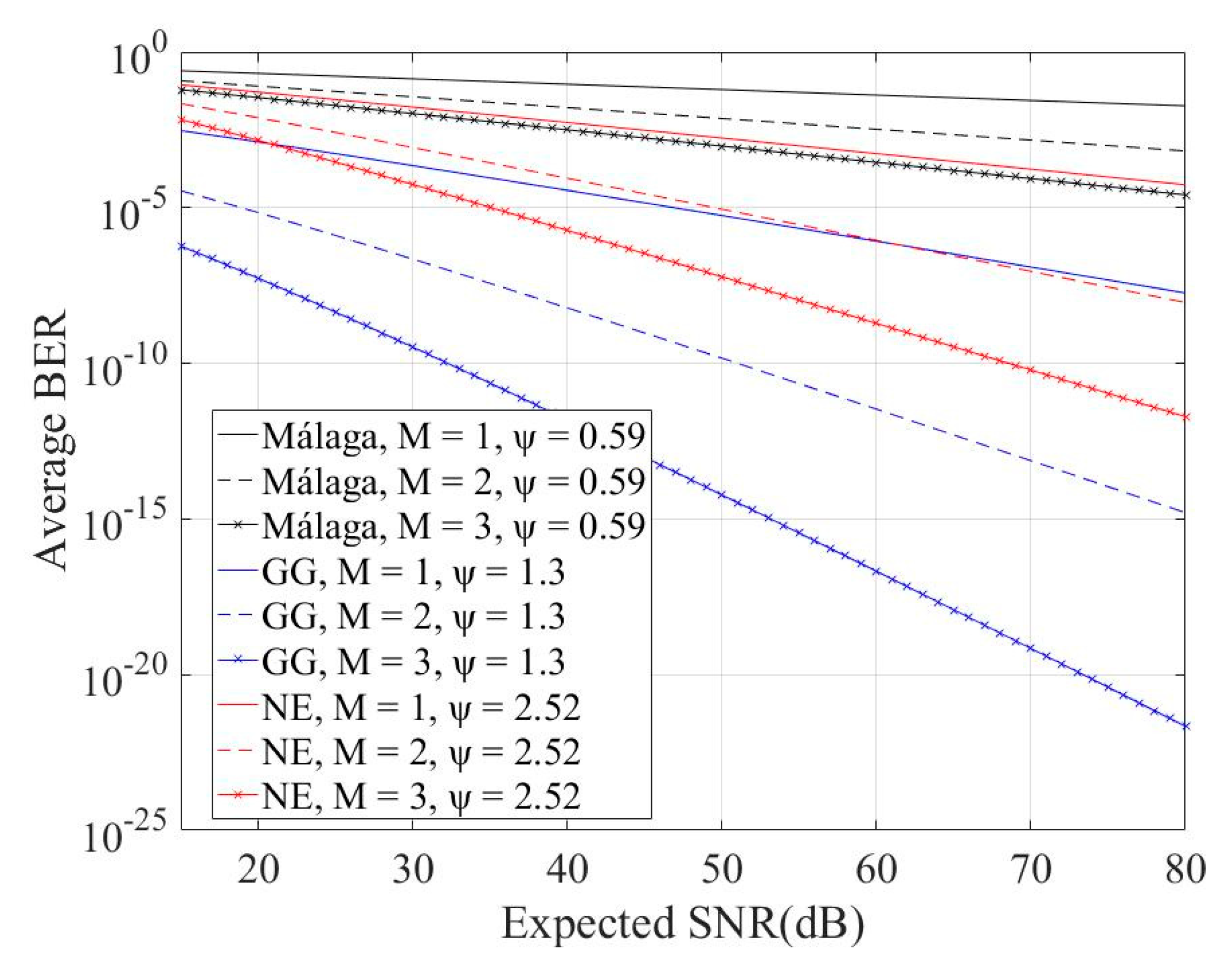
Figure 1 demonstrates the OP versus the normalized outage threshold for the cases, where the MG model approximates the GG or Málaga distributions, while Figure 2 shows the OP of NE cases, accompanied by the corresponding Monte Carlo simulations with 1 × 10⁹ samples. Figure 3 and Figure 4 illustrate the ABER versus electrical SNR for the same approximations, using OOK, and 4-PPM schemes respectively, with either wavelength, spatial, or time diversity. A significant decrease, in OP and ABER, for both modulation schemes is evident as the normalized outage threshold or the average electrical SNR increase, respectively, despite the stronger PE impact for the GG distribution, compared to the NE approximation. This is well argued, since the NE distribution describes saturated conditions of turbulence, while the GG one refers to weaker turbulence conditions, due to the selected values of a and β. In the scenario where the MG approximates the Málaga distribution, we consider even a stronger PE impact. Although the Málaga describes weaker turbulence conditions compared with the NE case, a decreased performance in both terms OP and ABER is observed since the strong PE effect dominates over turbulence. Moreover, the 4-PPM scheme is more efficient than OOK in all cases examined. Furthermore, in all scenarios it is clear that the SIMO system outperforms the system with only one transmission.
5. Conclusions
A SIMO FSO system, with wavelength, spatial, and time diversity, along with OOK or L-PPM modulation and OC method at the receiver side, operating over the combined effect of atmospheric turbulence and NZB-PEs, was investigated. In order to reduce the mathematical complexity of the derived expressions, a mixture composite channel model was adopted. Novel mathematical expressions of the OP and the ABER were deduced and appropriate numerical results were graphically depicted.
Author Contributions
Conceptualization, N.A.A., H.E.N., A.N.S., H.G.S. and G.S.T.; methodology, N.A.A., H.E.N. and H.G.S.; software, N.A.A. and A.N.S.; validation, N.A.A., H.E.N. and A.N.S.; formal analysis, N.A.A. and H.E.N.; investigation, N.A.A., H.E.N., A.N.S., H.G.S. and G.S.T.; resources, N.A.A., H.E.N., A.N.S., H.G.S. and G.S.T.; writing—original draft preparation, N.A.A., A.N.S.; writing—review and editing, H.E.N., H.G.S. and G.S.T.; supervision, H.E.N.; funding acquisition, H.E.N., G.S.T.
Funding
N.A.A. acknowledges that this research is co-financed by Greece and the European Union (European Social Fund- ESF) through the Operational Program «Human Resources Development, Education, and Lifelong Learning» in the context of the project, “Strengthening Human Resources Research Potential via Doctorate Research” (MIS-5000432), implemented by the State Scholarships Foundation (ΙΚΥ). HEN, A.N.S. and G.S.T. acknowledges the funding from the European Union’s Horizon 2020 research and innovation program under grant agreement No: 777596.
Conflicts of Interest
The authors declare no conflict of interest.
References
- Ghassemlooy, Z.; Arnon, S.; Uysal, M.; Xu, Z.; Cheng, J. Emerging optical wireless communications-advances and challenges. IEEE J. Sel. Areas Commun. 2015, 33, 1738–1749. [Google Scholar] [CrossRef]
- Khalighi, M.A.; Uysal, M. Survey on free space optical communication: A communication theory perspective. IEEE Commun. Surv. Tutor. 2014, 16, 2231–2258. [Google Scholar] [CrossRef]
- Boluda-Ruiz, R.; García-Zambrana, A.; Castillo-Vázquez, C.; Castillo-Vázquez, B. Novel approximation of misalignment fading modeled by beckmann distribution on free-space optical links. Opt. Express 2016, 24, 22635. [Google Scholar] [CrossRef] [PubMed]
- Varotsos, G.K.; Nistazakis, H.E.; Petkovic, M.I.; Djordjevic, G.T.; Tombras, G.S. SIMO optical wireless links with nonzero boresight pointing errors over m modeled turbulence channels. Opt. Commun. 2017, 403, 391–400. [Google Scholar] [CrossRef]
- Sandalidis, H.G.; Chatzidiamantis, N.D.; Karagiannidis, G.K. A Tractable model for turbulence- and misalignment-induced fading in optical wireless systems. IEEE Commun. Lett. 2016, 20, 1904–1907. [Google Scholar] [CrossRef]
- Gradshteyn, I.S.; Ryzhik, I.M. Special Functions. In Table of Integrals, Series, and Products, 7th ed.; Jeffrey, A., Zwillinger, D., Eds.; Elsevier (Academic Press): New York, NY, USA, 2008; pp. 859–1046. [Google Scholar]
- Jurado-Navas, A.; Maria, J.; Francisco, J.; Puerta-Notario, A. A Unifying Statistical Model for Atmospheric Optical Scintillation. In Numerical Simulations of Physical and Engineering Processes; InTech, 2011. Available online: https://www.intechopen.com/books/numerical-simulations-of-physical-and-engineering-processes/a-unifying-statistical-model-for-atmospheric-optical-scintillation (accessed on 18 May 2019).
- Varotsos, G.K.; Nistazakis, H.E.; Volos, C.K.; Tombras, G.S. FSO links with diversity pointing errors and temporal broadening of the pulses over weak to strong atmospheric turbulence channels. Optik 2016, 127, 3402–3409. [Google Scholar] [CrossRef]
- Ninos, M.P.; Nistazakis, H.E.; Tombras, G.S. On the BER performance of FSO links with multiple receivers and spatial jitter over gamma-gamma or exponential turbulence channels. Optik 2017, 138, 269–279. [Google Scholar] [CrossRef]
- Sandalidis, H.G.; Chatzidiamantis, N.D.; Ntouni, G.D.; Karagiannidis, G.K. Performance of free-space optical communications over a mixture composite irradiance channel. Electron. Lett. 2017, 53, 260–262. [Google Scholar] [CrossRef]
- Nistazakis, H.E.; Tombras, G.S. On the use of wavelength and time diversity in optical wireless communication systems over gamma-gamma turbulence channels. Opt. Laser Technol. 2012, 44, 2088–2094. [Google Scholar] [CrossRef]
- Chiani, M.; Dardari, D.; Simon, M.K. New exponential bounds and approximations for the computation of error probability in fading channels. IEEE Trans. Wirel. Commun. 2003, 24, 840–845. [Google Scholar] [CrossRef] [Green Version]
- Prudnikov, A.P.; Brychkov, Y.A.; Marichev, O.I. Definite Integral. In Integrals and Series: Special Functions; Gordon and Breach Science Publishers: Glasgow, UK, 1992; Volume 2, pp. 55–312. [Google Scholar]
Figure 1.
OP performance versus the normalized outage threshold for GG and Málaga cases.
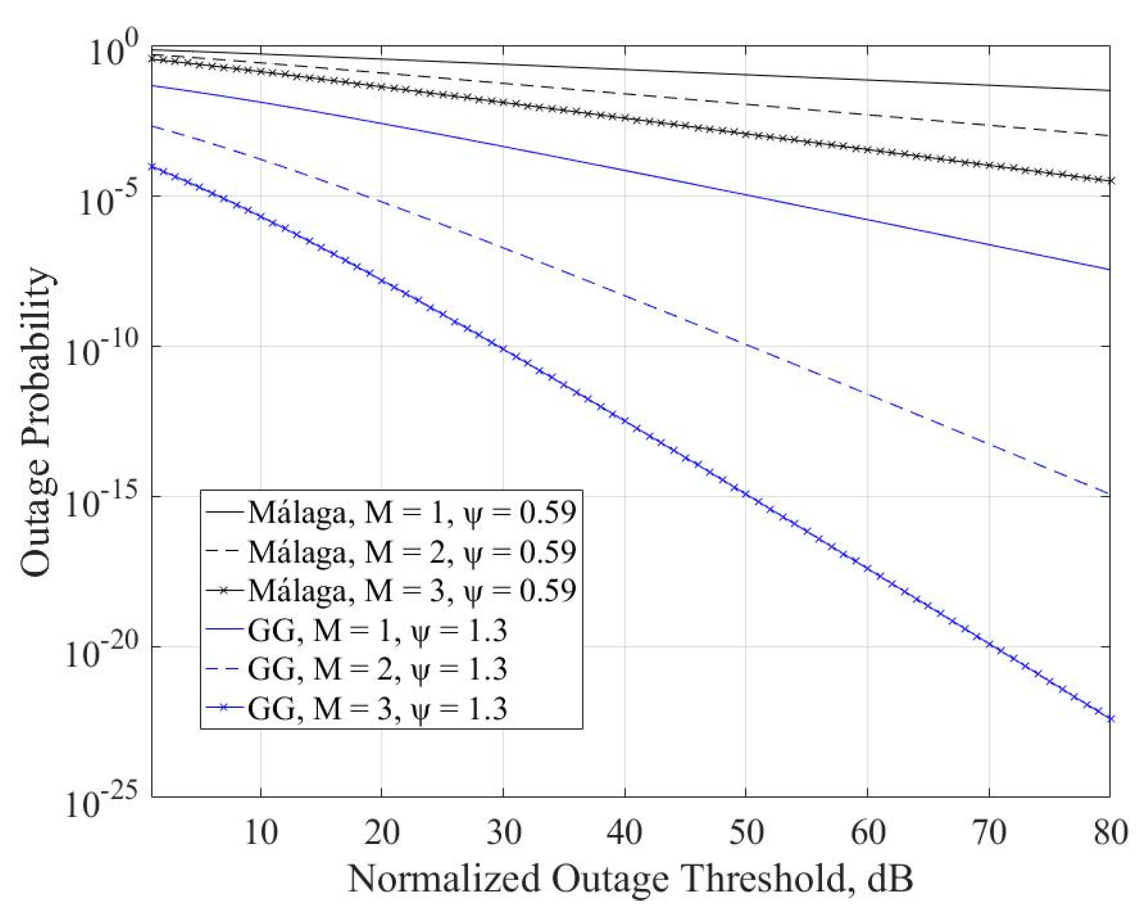
Figure 2.
OP performance versus the normalized outage threshold for NE case.

Figure 3.
ABER for OOK scheme versus the expected SNR.
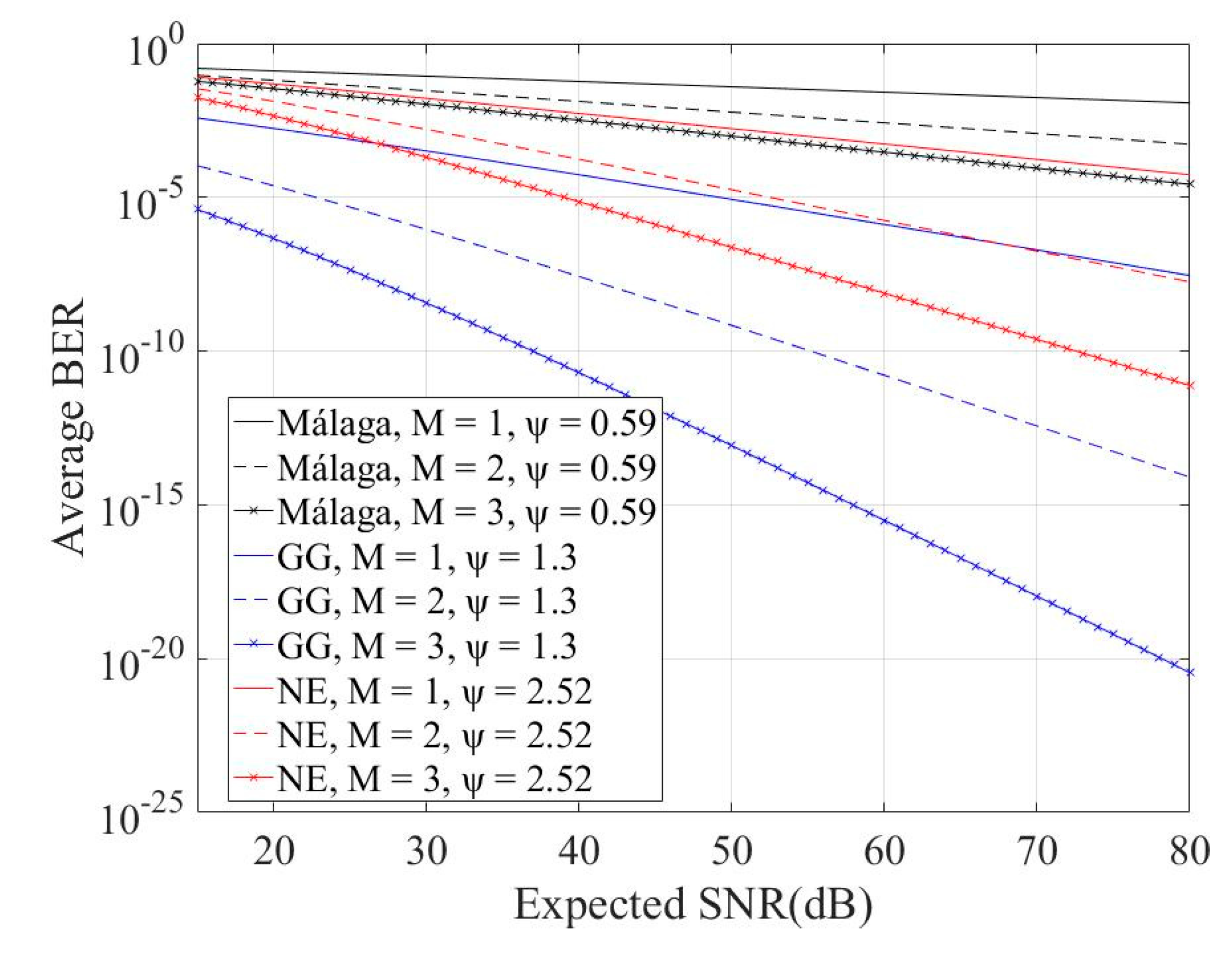
Figure 4.
ABER for 4-PPM scheme versus the expected SNR.

Table 1.
Values of turbulence and pointing errors parameters.
| Distributions | α or α’ | β or β’ | ψ | A0 | g |
|---|---|---|---|---|---|
| NE | - | - | 2.52 | 0.04 | 0.79 |
| GG | 2 | 5 | 1.3 | 0.04 | 1.21 |
| Málaga | 2 | 5 | 0.59 | 0.04 | 11.86 |
© 2019 by the authors. Licensee MDPI, Basel, Switzerland. This article is an open access article distributed under the terms and conditions of the Creative Commons Attribution (CC BY) license (http://creativecommons.org/licenses/by/4.0/).
Share and Cite
MDPI and ACS Style
Androutsos, N.A.; Nistazakis, H.E.; Stassinakis, A.N.; Sandalidis, H.G.; Tombras, G.S. Performance of SIMO FSO Links over Mixture Composite Irradiance Channels. Appl. Sci. 2019, 9, 2072. https://doi.org/10.3390/app9102072
AMA Style
Androutsos NA, Nistazakis HE, Stassinakis AN, Sandalidis HG, Tombras GS. Performance of SIMO FSO Links over Mixture Composite Irradiance Channels. Applied Sciences. 2019; 9(10):2072. https://doi.org/10.3390/app9102072
Chicago/Turabian StyleAndroutsos, Nikolaos A., Hector E. Nistazakis, Argyris N. Stassinakis, Harilaos G. Sandalidis, and George S. Tombras. 2019. "Performance of SIMO FSO Links over Mixture Composite Irradiance Channels" Applied Sciences 9, no. 10: 2072. https://doi.org/10.3390/app9102072
Note that from the first issue of 2016, this journal uses article numbers instead of page numbers. See further details here.