Fault Classification of Rotary Machinery Based on Smooth Local Subspace Projection Method and Permutation Entropy

1
Key Laboratory of Metallurgical Equipment and Control Technology, Wuhan University of Science and Technology, Ministry of Education, Wuhan 430081, China
2
Hubei Key Laboratory of Mechanical Transmission and Manufacturing Engineering, Wuhan University of Science and Technology, Wuhan 430081, China
*
Author to whom correspondence should be addressed.
Appl. Sci. 2019, 9(10), 2102; https://doi.org/10.3390/app9102102
Submission received: 24 March 2019
/
Revised: 10 May 2019
/
Accepted: 13 May 2019
/
Published: 22 May 2019
(This article belongs to the Special Issue Structural Damage Detection and Health Monitoring)
Abstract
:Collected mechanical signals usually contain a number of noises, resulting in erroneous judgments of mechanical condition diagnosis. The mechanical signals, which are nonlinear or chaotic time series, have a high computational complexity and intrinsic broadband characteristic. This paper proposes a method of gear and bearing fault classification, based on the local subspace projection noise reduction and PE. A novel nonlinear projection noise reduction method, smooth orthogonal decomposition (SOD), is proposed to denoise the vibration signals of various operation conditions. SOD can decompose the reconstructed multiple strands to identify smooth local subspace. In the process of projection from a high dimension to a low dimension, a new weight matrix is put forward to achieve a better denoising effect. Afterwards, permutation entropy (PE) is applied in the detection of time sequence randomness and dynamic mutation behavior, which can effectively detect and amplify the variation of vibration signals. Hence PE can characterize the working conditions of gear and bearing under different conditions. The experimental results illustrate the effectiveness and superiority of the proposed approach. The theoretical derivations, numerical simulations and experimental studies, all confirm that the proposed approach based on the smooth local subspace projection method and PE, is promising in the field of the fault classification of rotary machinery.
1. Introduction
Gear and bearing are very important parts in mechanical systems, because their working conditions can directly affect safety and stable operations. Therefore, it is of great significance to detect and diagnose their operating states [1,2,3,4]. The main denoising algorithms aim at one dimensional time domain vibration signals in the field of current mechanical signal noise reduction methods [5]. The vibration signals of rotary machinery have high computational complexity and large storage space, and many nonlinear or chaotic time series have an inherent broadband characteristic [6], which makes noise reduction so difficult. The nonlinear time series analysis method has been used in the fault diagnosis of rotary machinery. The analysis of vibration signal is vital for monitoring the operating condition of rolling bearings, and the accurate extraction of fault characteristic frequencies from vibration signals is particularly important [7].
In the process of monitoring rotating machinery, using signal processing methods to analyze and extract fault characteristic frequencies is becoming a common technique. Several signal processing methods, such as wavelet transform (WT) [8,9], independent component analysis (ICA) [10,11], empirical mode decomposition (EMD) [12,13], phase space reconstruction (PSR) [14], and sparse decomposition (SD) [15,16], are widely used in this field. In the phase space reconstruction, one dimensional time series is reconstructed to high dimensional phase space to explore its underlying dynamical characteristics, hidden in one dimensional space [17]. Tufillaro and Artuso et al. [18] explained the ways of calculating fractal dimension and entropy in the nonlinear series to measure the complexity and regularity of time series.
The proper orthogonal decomposition (POD) [19,20,21], which is also known as Karhunen-Loeve decomposition, has been widely applied to analyze nonlinear series fields as an effective tool in capturing the dominant modes and components. It is a statistical analysis technique in finding the coherent structures [22] in nonlinear data, which defines the optimum basis according to energy. The POD method has been advantageously applied in different fields, such as the stochastic finite element methods [23], the simulation of random fields [24], the damage identification [25], and the linear and nonlinear systems modal analysis [26]. In the nonlinear dynamics field, the POD is used to extract the dimensional information from an embedded attractor. In mechanical engineering and signal processing, the algorithm is conducted to identify subspaces [27] to obtain constrained clean trajectories in order to denoise the time series containing noises. Further studies lead to a modified decomposition called smooth orthogonal decomposition (SOD) [28,29,30], and it can be regarded as a projection of an ensemble of spatially distributed data. In smooth local decomposition, the one dimensional time series is reconstructed to high dimensional phase space, then noises in the data can be reduced by being projected to the tangent subspace [31]. The vector directions of the projection can make sure the variance is as maximum as possible, and the motions obtaining along these vector directions are the smoothest in terms of time. The vector directions can be defined as the eigenvectors of the eigenproblem [32] from the correlation matrices of the random field and the relevant time derivative. The basic idea of SOD derived from the proposed optimal tracking approach [33], and was formulated as a modal analysis tool. Then the smooth orthogonal approach [34] was evolved in terms of time continuous stationary random vector processes, and it was extended to time continuous and non-stationary random vector processes. During the process, the smooth orthogonal projection from a high dimension phase space to a low dimension one, a new weight matrix is put forward to achieve a better denoising effect by adding back the bias in this paper, which has been proved effective after multiple experiments.
Christoph Bandt et al. [35] proposed the concept of the average entropy parameter in the application of measuring the complexity of one dimensional time series, namely permutation entropy (PE). It was an algorithm study about describing irregular and nonlinear systems [36], which cannot, or are hard to be, quantitatively described, in a relatively simple way. The PE has the advantages of simple calculation, strong anti-noise ability, and high sensitivity to signal change. The entropy derived methods can also be applied to the weak signal detection [37,38], and the detection of the dynamic mutation of the complex system.
When an abnormal failure or different kinds of faults occur in gear and bearing parts during their operation process, the influence of the nonlinear factors and signal complexity are different [39,40,41,42]. So the vibration signals obtained from the mechanical system will also change, resulting in different values of PE. The PE is essentially used to describe the aggregation extent of phase vectors [43] in the high dimensional space. As for gear and bearing parts, different fault types have different degrees of faults. The smaller value of entropy means the lower complexity of fault signals, namely, the more serious the fault type is, the smaller its entropy, owing to a better predictability of fault signals. Thus, PE can be adopted to classify the different kinds of gear and bearing faults.
This paper proposes a novel approach to conduct fault classification of gear and bearing signals, based on the smooth local subspace projection denoising and PE. The proposed novel weighting matrix is verified to be better than the existing weight matrices. The organization of this paper is as follows: Section 2 introduces the basic principles and characteristics of a smooth local decomposition and an algorithm, as well as the concept of PE. It then describes the theory of the fault classification method based on the smooth local subspace projection and PE. Section 3 introduces the numerical experiments of the smooth local subspace projection, and simulation researches of PE, which both can prove the effectiveness of the algorithm. Section 4 presents the processing of Case Western Reserve University Bearing Data and its applications to gear signals of the Drivetrain Diagnostics Simulator, in order to verify the validity of the proposed approach described in this paper. The conclusions of the studies and necessary discussions are given in Section 5.
2. The Theory of the Smooth Local Subspace Projection Noise Reduction and PE
2.1. The Theory of Smooth Local Subspace Projection Noise Reduction Method
Smooth projection noise reduction [28,29,30] which is based on SOD, is applied to phase space reconstruction of the noisy signals generated by mechanical systems. The basic principle is that noises can divulge to a higher dimensional phase space of the tangent space of its attractor. Here, the data are embedded into a higher dimensional space, then are projected to dimensional tangent subspaces to achieve the purpose of denoising. The limitation of trajectories on the subspace strengthens the smoothness of the time series which has been filtered, thus obtaining a better denoising effect. The time series with noises is embedded into a dimensional phase space, which is composed of vector value trajectories generated by a delay coordinate, as shown in Equation (1).
where τ is delay time, which is usually determined by using the average mutual information method [44]. The selection of global embedding dimension and tangent subspace dimension is one of the most important steps. False nearest neighbor method is often used to estimate minimum embedding dimension . In addition, the embedding theorem [45] provides a method for choosing the minimum embedding dimension: The minimum embedding dimension should be two times larger than the fractal dimension of its attractor.
2.2. Local Projection Subspace
In the local projection denoising algorithm [46,47], as for each point in reconstructed dimensional phase space, temporarily uncorrelated neighborhood points are determined. Local subspace projection denoising method deals with short strands in the reconstructed phase space trajectories. These strands are composed of reconstructed phase space points of continuous time, among which is a small natural number. Namely that each reconstructed point has an associated strand, as shown in Equation (2).
Meanwhile nearest neighbor strands including constitute into . These strands are constructed by seeking the nearest neighbor points of . Smooth local decomposition is conducted to every strand to obtain the corresponding dimensional smooth approximation to , the filtered point is determined by the weighted average of points in the smooth strands. Then, the filtered time series is obtained in local projection denoising. The algorithm can be iterated many times to further smooth and filter the noise time series to obtain better denoising effect.
2.3. SOD and Data Projection
SOD [34] aims at obtaining a smooth low dimensional approximation of a high dimensional dynamic process, and it considers the time characteristics and space characteristics, whereas POD only considers the geometrical or topological properties of data, and does not take any temporal characteristics of time series into account. For example, when y is defined as a field of d state variables, assume that this field happens to take samples in instantaneous time. The data can be formed into an matrix , so is the sample of the th moment from the th state variable, and the mean value of each row of matrix is assumed as 0. Then a linear coordinate transformation of this matrix is conducted as shown in Equation (3).
where each row of is a new smooth orthogonal component, smooth projection modes [29] are decided by the rows of . In the process of above change, time coordinates needs to be considered in which is ranked by the roughness. Then SOD is realized through the following generalized characteristic value problem, as shown in Equation (4).
where and are the auto-covariance matrix of state variables and their time derivatives. The characteristic value are smooth orthogonal characteristic values.
The above Equation (4) can be realized by the following matrix, as shown in Equation (5).
where smooth, orthogonal modes and smooth, orthogonal components are determined by the rows of and respectively, and smooth, orthogonal characteristic values are determined by the term by term division of the diagonal matrix and . The dimensional smooth approximation of can be obtained by retaining rows of matrix and , meanwhile the matrix is reduced to order accordingly. The projection of in dimensional smooth subspace is the purpose. The dimensional projection is embedded into dimensional space by using the corresponding matrices, as shown in Equation (6), which involves with three matrix transformations.
Then the matrix can be obtained by the following Equation (7).
The main steps of this smooth local subspace projection method are given in Table 1.
2.4. Smooth Local Subspace Projection Method
In the process of that, original strands are projected to a low dimensional smooth subspace, weighting matrix [34] is used to consider the bias during the projection. The in the means the number of points in each strand. There are three types of weighting functions which respectively are, the comb weighting function, the tent weighting function and the exponential weighting function, as in Equations (8)–(10).
There are many denoising evaluation indicators. Visual identification is used at early stages until contemporary peak ratios, margin, and kurtosis can be regarded as evaluation indicators of denoising. The most basic indicator is the signal to noise ratio (SNR), which is adopted here. In addition to that, mean square error (MSE) and Cm, which represents similarity, are also used to evaluate the effectiveness of the proposed method, as shown in Equations (11)–(13) respectively.
where is mean power of the original signal, and is mean power of the Lorenz signal with noises, is the original signal without noises, is the denoised signal after iteration denoising of SOD. To verify the effectiveness of the proposed method, the following simulated signal is adopted for simulation research.
where Hz, Hz, and denotes the added Gaussian white noise, with variance of 1, and mean of 0. The above three evaluation indicators can be utilized to signify the validity of the smooth local subspace projection denoising method intuitively. The above three factors have different effectiveness towards the smooth local subspace projection method, as shown in Figure 1, Figure 2 and Figure 3.
It can be seen from Figure 1, Figure 2 and Figure 3 that the comb weighting function, tent weighting function and exponential weighting function can achieve a proper denoising effect during the iterations of the smooth local subspace projection method, but three weighting functions achieve different denoising effects. Thus, it occurred to the authors that it is possible to find a better weighting function which can be applied to smooth local subspace projection method.
After multiple simulation researches conducted by authors, a new weighting matrix function is put forward, namely the logarithmic weighting function, as shown in Equation (15).
The denoising effectiveness of above four kinds of weighting matrices can be shown as Figure 4, Figure 5 and Figure 6.
It can be seen from Figure 4, Figure 5 and Figure 6 that the logarithmic weighting function has the better denoising effect than the abovementioned three weighting functions during the process that the high dimensional data are projected to the lower dimensional subspace. The simulation researches demonstrate the effectiveness and superiority of the proposed weighting function, hence it can be applied in the fault classification of rotary machinery.
2.5. Definition of PE
Assuming a one dimensional time series , and that it can be embedded into a high dimensional phase space by using phase space reconstruction, then the following matrix in Equation (16) can be obtained.
where , and are embedding dimension and delay time respectively, . Each row in the matrix can be regarded as a reconstructed component, and there is a total of reconstructed components.
In the reconstructed matrix is realigned in ascending order, and represent indices of each of the elements in the column of reconstructed components, which can be described in Equation (17).
If there are equivalent values in reconstructed components, then the elements should be aligned according to the values of and . When there are two of equal value, and in the following situation, it can be ranked as in Equation (18) in order to solve the same value situation.
It can be obtained from above that, for any time series, each row in the reconstructed matrix can generate a set of symbolic sequence, as shown in Equation (19).
where , and . There is a total of kinds of different mapping symbol sequences of dimensional phase space, and symbol sequence is one of them. The probability of each symbol sequence is respectively, the PE [35] of kinds of different symbol sequences of a time series is defined according to information entropy, as shown in Equation (20).
The size of value represents the random degree of the time series: The smaller value of means the more regular of the time series, and the larger value of means the more random of the time series. The change of can show and enlarge the detail changes of time series. In gear and bearing fault diagnosis, the more serious the fault type is, the more regular of the one dimensional time series is, the smaller PE will be.
2.6. Proposed Fault Classification Method Based on the Smooth Local Subspace Projection Denoising Method and PE
In this paper, a novel method of applying PE in the fault classification of rotary machinery based on the smooth local subspace projection denoising method is proposed. After experimental studies, it can be obtained that the smooth projection denoising method has an obvious noise reduction effect towards a nonlinear and nonstationary signal. Thus, the smooth local subspace projection method can be well applied to a variety of mechanical fault signals. As for gear and bearing parts, different fault types correspond to different fault degrees. The smaller entropy means the less complexity of fault signal type, namely that when the fault type is more serious, the fault signal has better predictability, and its entropy will be smaller. From all above theoretical derivations, the smooth local subspace projection method can be used to denoise gear and bearing fault signals, and PE is utilized to the classification of different faults. The basic idea of the proposed method is illustrated in Figure 7.
3. Numerical Experiments
In order to study the effectiveness of the smooth local subspace projection method applying to mechanical fault signal analysis, Lorenz model [48] and frequency modulation (FM) signals [49] are adopted to assess the performance of the algorithm. The Lorenz model is one kind of typical nonlinear dynamic signals, and frequency modulation signals also usually exist in mechanical fault signals [50,51]. Hence, it is meaningful to analyze these two kinds of simulated signals to verify the effectiveness of this denoising algorithm.
3.1. Lorenz Signal Simulation Research
Lorenz equation is one kind of typical nonlinear dynamic problem. The following signal is used in the simulation research, all variables of which are dimensionless.
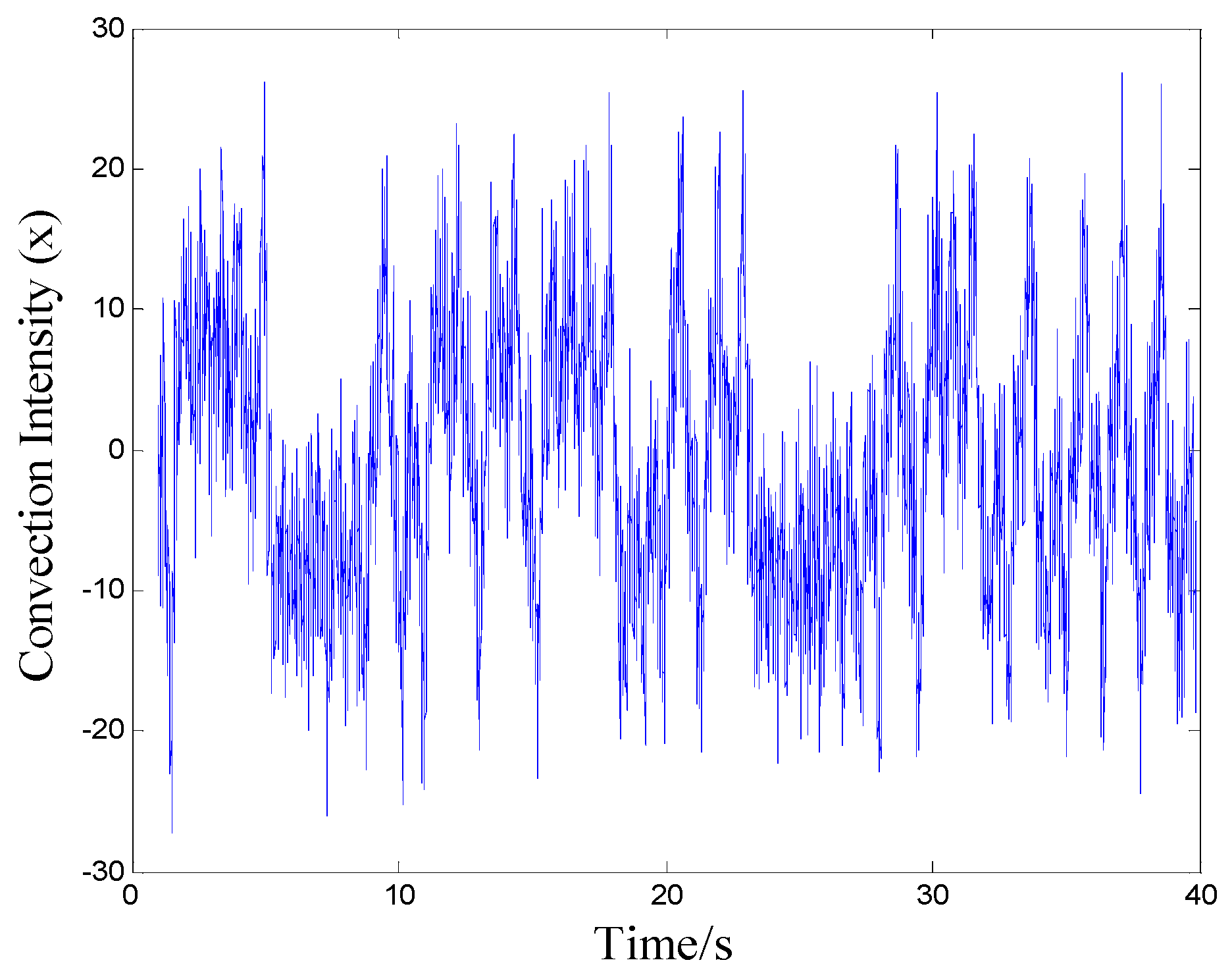
where denotes convection intensity, denotes convection caused by horizontal temperature difference, represents variables related to vertical temperature difference, is the Prandtl number, is the Rayleigh number, and represents parameters related to container size. A Lorentz signal with parameters of , , is constructed. The time series obtained from 100 Hz sampling frequency is used to analyze the effectiveness of the method under the condition of superimposing Gauss white noise. Gaussian white noise [52] amplitudes accord with Gaussian distribution, and its power spectral density uniformly distributes, so it is very appropriate for simulation analysis. Here the magnitude of superimposed Gaussian white noise is 5 dB. The first 40 s time domain plot of component of Lorenz signal is shown in Figure 8 and Figure 9.
After calculating the fractal dimension of the main attractor of Lorenz signal, and are selected as the embedding dimension and local embedding dimension, respectively [34]. Then the SOD method is conducted to denoise this Lorenz signal with noises. The domain plot of the component of the denoised signal is shown in Figure 10. The phase space reconstruction of original signal, superimposed noises signal, and 7 times iteration denoised signal, are shown in Figure 11.
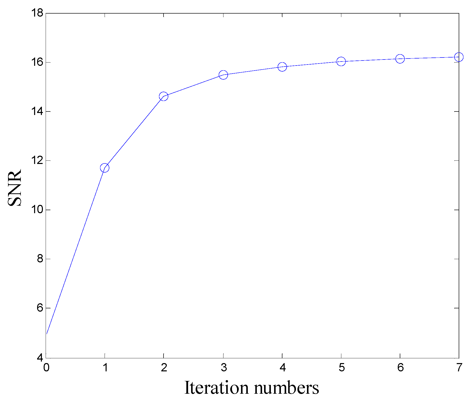
The SNR, Cm, and MSE values change along with iterations, and can be shown in Figure 12, Figure 13 and Figure 14 respectively.
It can be seen from various parameters’ value changes of the above figures, that the SOD has a significant effect towards a typical nonlinear signal, such as the Lorenz signal, in denoising. After 7 times SOD noise reduction algorithm iterations, SNR changed from 5 to 16.2009, Cm changed from 0.8726 to 0.9886, MSE changed from 21.4739 to 1.6129, so the effectiveness of the method can be regarded as good. It can be seen from the simulation researches that this SOD algorithm is suitable for denoising nonlinear and nonstationary signals. Since mechanical vibration signals have strong nonlinear and nonstationary characteristics, it can be concluded that the proposed smooth local subspace projection method based on SOD can be applied in denoising the mechanical vibration signals.
3.2. FM Signal Simulation Research
FM signals usually exist in vibration signals of mechanical operation signals. In this paper, the FM signal is adopted to conduct the simulation analysis of noise reduction, in order to verify whether the algorithm is suitable for FM signals, namely mechanical signals. The simulation FM signal is shown in Equation (22).
The sampling frequency of the above signal is 4096 Hz, and the sampling point is 4096, with the addition of Gaussian white noise, the SNR of which is 2. The time domain plots of the original signal and our noisy signal are shown in Figure 15 and Figure 16. The time domain plot of the denoised FM signal with noises is shown in Figure 17.
It can be seen from Figure 15, Figure 16 and Figure 17 that the proposed smooth local subspace projection method can achieve a good denoising result. There is no extra noise in the denoised signal in time, three evaluation indicators of SNR, Cm and MSE can be utilized to measure the effectiveness of the smooth local subspace projection denoising method quantitatively. The SNR, Cm, and MSE values change along with iterations, and can be shown in Figure 18, Figure 19 and Figure 20, respectively. Furthermore, to show the effectiveness of the proposed approach, different noise levels for the FM signal are adopted to verify its denoising effect using the logarithmic weighting function. The values of three indicators of denoising performance are given in Table 2.
It can be seen from Figure 18, Figure 19 and Figure 20 that the FM signal is denoised by the proposed approach effectively, according to the three denoising indicators mentioned above. Furthermore, it can be seen from Table 2 that the proposed approach can achieve a good denoising effect under the condition of different added noise levels. Hence, it can be concluded from the simulation researches that the proposed smooth local subspace projection method based on SOD can achieve a good denoising effect towards FM signals. Owing to the reason that the mechanical vibration signals usually contain the characteristics of FM signals, the proposed approach can be applied to deal with mechanical vibration signals.
3.3. Simulation Research of PE
In order to verify the validity of applying PE to the detection of nonlinear signals, the FM signal is adopted to conduct simulation researches and to calculate the PE. The following FM signal in Equation (23) is applied in the simulation.
where the sampling frequency is of 1024 Hz, and the sampling time is 3 s. A Gaussian white noise signal is superimposed on the FM signal between 1 to 2 s. It aims at simulating the abnormal condition of mechanical parts. Through analyzing the noisy FM signal, the validity of PE applying to gear and bearing classification can be verified. The time domain plot of FM signal locally superimposed by Gaussian white noise is shown in Figure 21.
The above long time series is divided into several subsequences of length , and the cutoff point of subsequences corresponds to the third second moment of sampling time. These subsequences employ overlapping case, namely that each subsequence moves backward 20 data points to get the next subsequence. Then the PE of each subsequence is calculated, and its value is assigned to the middle data point of the subsequence. If the value of is too small, the calculated results will lose statistical significance. Meanwhile, in order to detect the change of signal accurately, the value of also cannot be too large. After comparison analysis of several times simulation experiments, here , , = 300 are adopted in the simulation experiment. The calculated results are shown in Figure 22.
It can be seen from the above figure that the PE values increase after the noise signal is superimposed on the FM signal, which results in less volatility and smooth variation of PE values, and the results indicate that the FM signal superimposed with noise is more random than the original FM signal, resulting in the bigger PE value. When noise disappears, this FM signal becomes regular again, and then PE values decrease to the previous level. From the simulation experiments, it can be concluded that, as for a given signal of random time series, mutation and status changes of signal will lead to a great change of PE value. Therefore, PE can be applied to mutation detection and state recognition, and thus can be adopted in gear and bearing fault classification.
4. Applications to Gear and Bearing Fault Classification
4.1. Application to Processing of Case Western Reserve University Bearing Data
Through numerical simulations, the proposed method based on the smooth local subspace projection method and PE can be applied to the signal which contains a frequency modulated signal in this section. The fault bearing data from the Case Western Reserve University Bearing Data Center Website [53] is used to verify the proposed method. The website provides a large collection of experimental bearing data that are related to faulty bearings, and among those, the data for faulty bearings are acquired by using electric spark machining. In this paper, inner race, ball, and outer race fault data of rolling bearings are adopted. The sampling frequency in the experiment is 12000 Hz, and the rotational speed is 1730 rpm. Experimental fault bearing type is 6205-2RS JEM SKF, and its specific parameters are shown in Table 3.
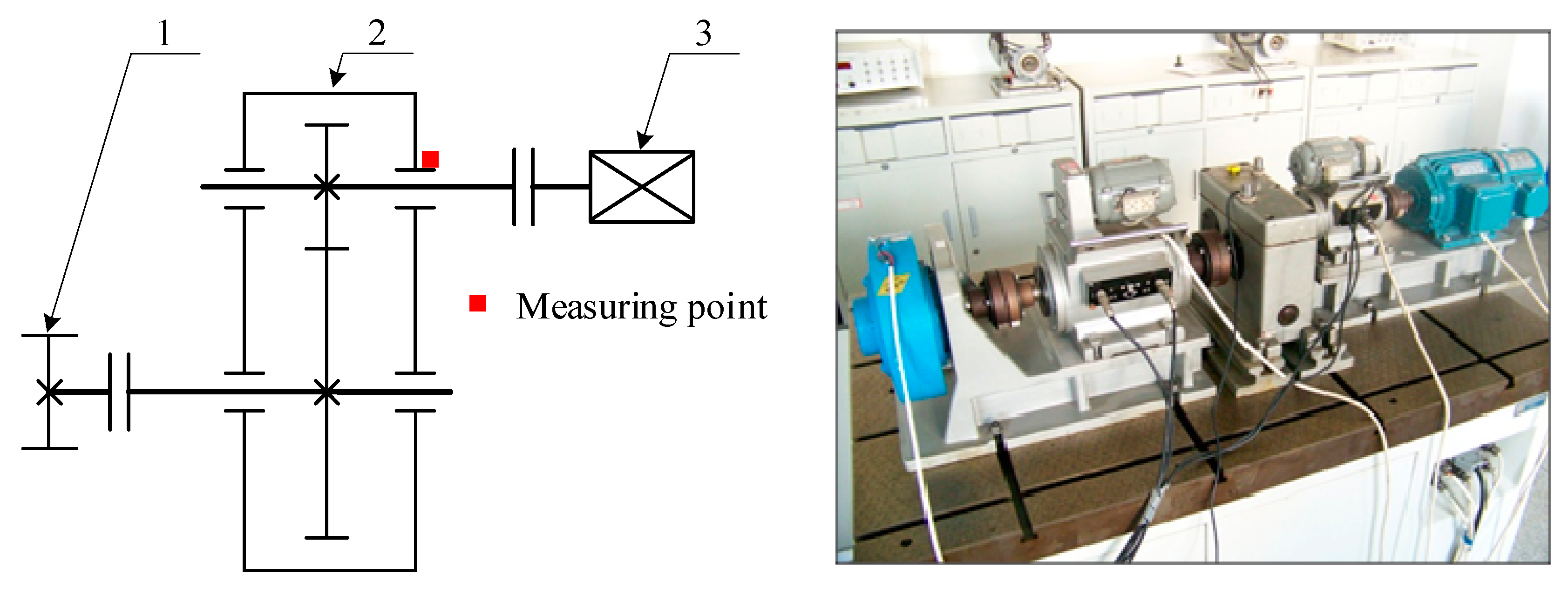
The test equipment of Case Western Reserve University (Cleveland, OHIO, USA) includes two motors, a coupling (containing torque sensor and encoder), and other related devices. An accelerometer is placed on the testing site to collect the acceleration signal that can be used for bearing fault analysis. The schematic diagram of a signal acquisition device and a picture are shown in Figure 23.
The collected signals, such as rolling bearings of defect on inner race, ball and outer race, contain a lot of noises, so it is difficult to classify the fault conditions of rolling bearing. The time domain plots of one set of gear signals are shown in Figure 24, Figure 25 and Figure 26.
It can be seen from Figure 24, Figure 25 and Figure 26 that the spectral analysis of these groups of signals cannot show the difference between different kinds of rolling bearing faults. Hence, the smooth local subspace projection method is applied to denoise 12 groups of signals for 10 times iteration denoising, and PE values of original vibration signals and denoised vibration signals are calculated, to conduct a fault classification of rolling bearings.
Through the permutation entropies of original signals and denoised signals above, it can show that before the smooth local subspace projection denoising, the PE values of one working condition are not distinguished from another working condition. All the PE values are aliasing, as shown in Figure 27. However, after the bearing vibration signals are denoised by the local projection method, the entropies of gear signals of four kinds of working conditions are distinguished very clearly. As shown in Figure 28, the PE values of the vibration signals of a ball defect bearing are the smallest, in range from 3.26 to 3.58, and their mean value is 3.34; the PE values of vibration signals of an inner race defect range from 3.64 to 3.78, and their mean value is 3.70; the PE values of vibration signals of the outer race defect range from 3.99 to 4.23, and their mean value is 4.12. The PE values of different fault types have different mean values and ranges, which can be applied to classify different kinds of mechanical fault signals. Hence, it can come to a conclusion that rolling bearings with different kinds of defect can be classified by the proposed method based on the proposed smooth local subspace projection method, using the logarithmic weighting function and PE. To sum up, the application researches demonstrate the effectiveness of the proposed method in the fault classification of rolling bearings.
4.2. Application to Drivetrain Diagnostics Simulator
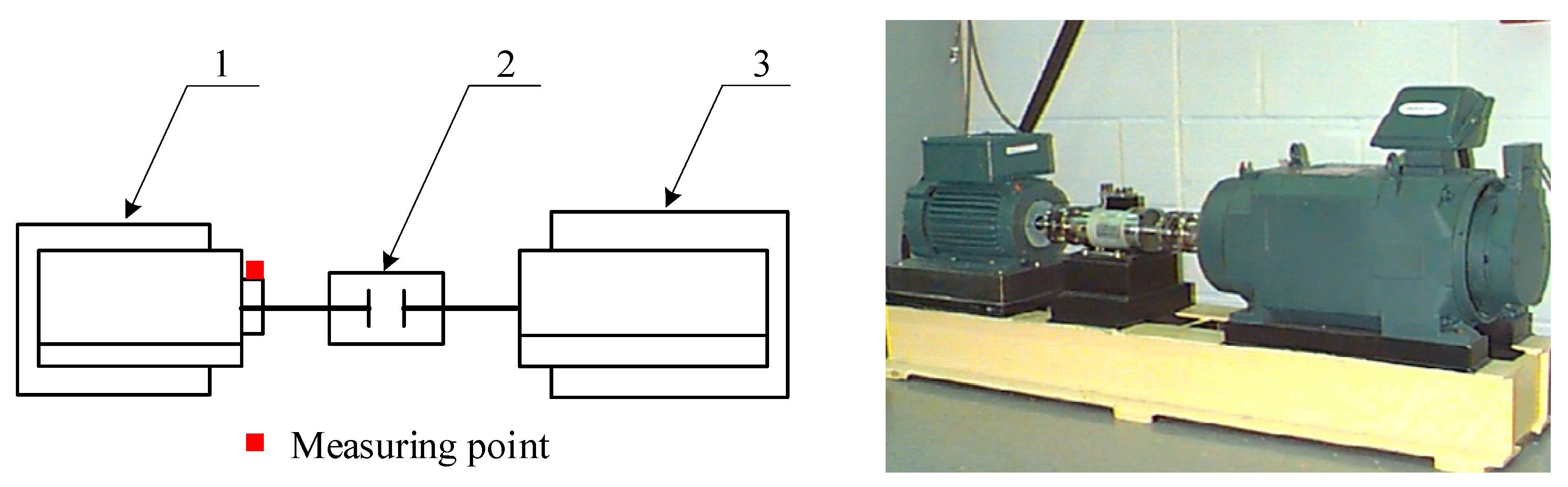
Through simulation researches, the proposed fault classification method based on the smooth local subspace projection and PE can be applied to the Gear signals. Owing to unqualified manufacture or improper manipulation, different kinds of gear faults would occur during the operation process. In the studies of this paper, the collected different fault signals of the Drivetrain Diagnostics Simulator are adopted to verify the effectiveness of the proposed method. The experimental apparatus has a single stage of gear transmission; the small gear is installed on the input shaft which tooth , the big gear is installed on the output shaft which tooth . The module of gears is 3. The load is generated by the magnetic powder brake, and the acceleration sensor is installed on the bearing pedestal of the input shaft in a vertical direction. Under different working conditions, several group signals, such as normal gear, broken tooth, wearing and circular pitch error gear vibration signals, were collected. There is a significant crack in the root of the broken tooth, the depth account tooth thickness of 2/5, and there is a distinct wear on the gear surface of the wearing tooth. The specific parameters of test conditions are as follows: The speed of high speed shaft is 363 r/min, and the load is 0 when the apparatus is idle, the sampling frequency and time are 2000 Hz and 3s respectively, so each set of data has 6000 sampling points. The experimental apparatus and its schematic diagram are shown in Figure 29. The apparatus contains a variable speed drive, a single stage gear transmission, and a magnetic powder brake.
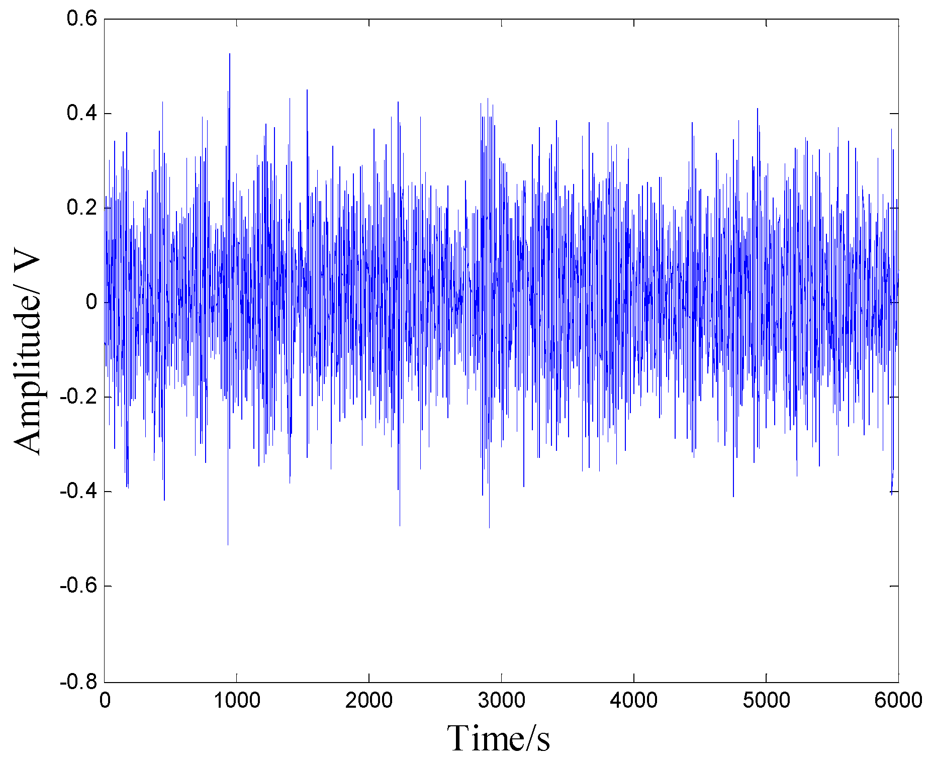
Since this apparatus is small, and has a high rigidity, the collected signals such as normal gear, broken tooth, wearing and circular pitch error signals, are all affected by vibration of the apparatus foundation bolts. The time domain plots of one set of gear signals are shown in Figure 30, Figure 31, Figure 32 and Figure 33. The spectral analysis of these groups of signals cannot show clear differences between different kinds of faults.
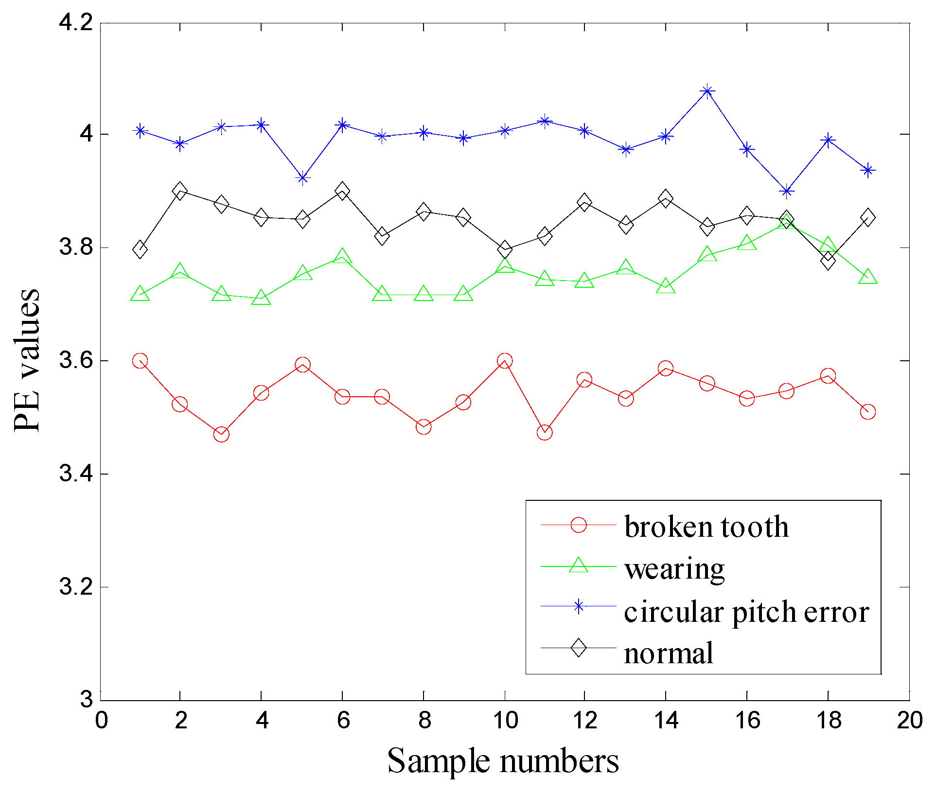
The smooth local projection method is applied to denoise 19 groups of signals for 10 times iteration denoising, and PE values of original vibration signals and denoised vibration signals are calculated, so as to conduct fault classification. The PE values of the original vibration signals and denoised vibration signals are shown in Figure 34 and Figure 35, respectively.
Through the PE values of original signals and denoised signals above, it can show that before the smooth local subspace projection denoising, the PE values of one working condition are not distinguished from another working condition. All the PE values are aliasing, as shown in Figure 34. However, after the gear vibration signals are denoised by the local projection method, the entropies of gear signals of four kinds of working conditions are distinguished very clearly. As shown in Figure 35, the permutation entropies of vibration signals of broken gears are the smallest, ranging from 3.47 to 3.60, and their mean value is 3.54; the permutation entropies of the vibration signals of wearing gear range from 3.71 to 3.84, and their mean value is 3.75; the permutation entropies of vibration signals of normal gear range from 3.78 to 3.90, and their mean value is 3.85; the permutation entropies of circular pitch error gears are the biggest, and range from 3.90 to 4.08, and their mean value is 3.99. The PE values of different fault types have different mean value and range, which can be applied to classify different kinds of mechanical fault signals. Hence, gears with different kinds of defects can be classified by the proposed method based on the proposed smooth local subspace projection method using the logarithmic weighting function and PE. To sum up, the application researches demonstrate the effectiveness of the proposed method in the fault classification of gears.
5. Conclusions
The research work in this paper elaborates on the theoretical effectiveness of the proposed method based on the smooth local subspace projection and PE. The new weight matrix also proves to be better than the existing weight matrices after being verified by repeated simulation researches. Through numerical simulations, the effectiveness of the smooth local projection denoising method can be verified, also the effectiveness of applying PE into the fault classification of mechanical signals. Through the applications to gear signals of the Drivetrain Diagnostics Simulator and the processing of Case Western Reserve University Bearing Data, multiple groups gear and bearing signals of different conditions are analyzed, in order to make the previous aliasing PE values into regular different PE mean value and ranges, and different fault types can be clearly classified. The results of numerical simulations and application researches demonstrate the significance of the proposed method in the field of fault classification. Hence, it can be concluded that gears and rolling bearings can be classified by the proposed novel smooth local subspace projection method, using the logarithmic weighting function and PE in this paper. The proposed method can effectively classify the fault modes, which is very beneficial to fault diagnosis of rotary machinery. From all above, it clearly indicates that the proposed method is a successful exploration, and it is very promising in the field of fault classification of rotary machinery.
Author Contributions
Y.L. conceived the study and providing valid criticism. L.X. performed the statistical analysis, discussed results and wrote the manuscript. G.F. contributed to data collection and analysis. All authors read and approved the manuscript.
Funding
This research was funded by National Natural Science Foundation of China under Grant No. 51875416 and No. 51475339, and Natural Science Foundation of Hubei Province under Grant No. 2016CFA042.
Acknowledgments
The authors appreciate the free download of the original bearing failure data and one photo picture provided by Case Western Reserve University Bearing Data Center Websit.
Conflicts of Interest
None of the authors have conflicts of interest in relation to this study.
References
- Caesarendra, W.; Pratama, M.; Kosasih, B.; Tjahjowidodo, T.; Glowacz, A. Parsimonious Network Based on a Fuzzy Inference System (PANFIS) for Time Series Feature Prediction of Low Speed Slew Bearing Prognosis. Appl. Sci. 2018, 8, 2656. [Google Scholar] [CrossRef]
- Yuan, N.; Yang, W.; Kang, B.; Xu, S.; Wang, X. Laplacian Eigenmaps Feature Conversion and Particle Swarm Optimization-Based Deep Neural Network for Machine Condition Monitoring. Appl. Sci. 2019, 8, 2611. [Google Scholar] [CrossRef]
- Kuai, M.; Cheng, G.; Pang, Y.; Li, Y. Research of Planetary Gear Fault Diagnosis Based on Permutation Entropy of CEEMDAN and ANFIS. Sensors 2018, 18, 782. [Google Scholar] [CrossRef]
- Lv, Y.; Yuan, R.; Shi, W. Fault Diagnosis of Rotating Machinery Based on the Multiscale Local Projection Method and Diagonal Slice Spectrum. Appl. Sci. 2018, 8, 619. [Google Scholar] [CrossRef]
- Bozchalooi, I.S.; Liang, M. A joint resonance frequency estimation and in-band noise reduction method for enhancing the detectability of bearing fault signals. Mech. Syst. Signal Process. 2008, 22, 915–933. [Google Scholar] [CrossRef]
- Arnel, H.; Brown, R.; Kadtke, J. Prediction and system identification in chaotic nonlinear systems: Time series with broadband spectra. Phys. Lett. A 1989, 138, 401–408. [Google Scholar]
- Lee, S.K.; White, P.R. The enhancement of impulsive noise and vibration signals for fault detection in rotating and reciprocating machinery. J. Sound Vib. 1998, 217, 485–505. [Google Scholar] [CrossRef]
- Jiang, T.; Li, Y.; Song, G. Detection of High-Strength Bolts Looseness Using Lead Zirconate Titanate Due to Wavelet Packet Analysis. Earth Sp. 2018, 1069. [Google Scholar] [CrossRef]
- Yang, W.; Kong, Q.; Ho SC, M.; Mo, Y.L.; Song, G. Real-Time Monitoring of Soil Compaction Using Piezoceramic-Based Embeddable Transducers and Wavelet Packet Analysis. IEEE Access 2018, 6, 5208–5214. [Google Scholar] [CrossRef]
- Chen, X.; Ma, D. Mode Separation for Multimodal Ultrasonic Lamb Waves Using Dispersion Compensation and Independent Component Analysis of Forth-Order Cumulant. Appl. Sci. 2019, 9, 555. [Google Scholar] [CrossRef]
- Fang, L.; Sun, H. Study on EEMD-Based KICA and Its Application in Fault-Feature Extraction of Rotating Machinery. Appl. Sci. 2018, 8, 1441. [Google Scholar] [CrossRef]
- Lv, Y.; Yuan, R.; Song, G. Multivariate empirical mode decomposition and its application to fault diagnosis of rolling bearing. Mech. Syst. Signal Process. 2016, 81, 219–234. [Google Scholar] [CrossRef]
- Yuan, R.; Lv, Y.; Song, G. Multi-fault diagnosis of rolling bearings via adaptive projection intrinsically transformed multivariate empirical mode decomposition and high order singular value decomposition. Sensors 2018, 18, 1210. [Google Scholar] [CrossRef] [PubMed]
- Wang, G.F.; Li, Y.B.; Luo, Z.G. Fault classification of rolling bearing based on reconstructed phase space and Gaussian mixture model. J. Sound Vib. 2009, 323, 1077–1089. [Google Scholar] [CrossRef]
- Liang, L.; Shan, L.; Liu, F.; Niu, B.; Xu, G. Sparse Envelope Spectra for Feature Extraction of Bearing Faults Based on NMF. Appl. Sci. 2019, 9, 755. [Google Scholar] [CrossRef]
- Zhang, Y.; Tong, S.; Cong, F.; Xu, J. Research of feature extraction method based on sparse reconstruction and multiscale dispersion entropy. Appl. Sci. 2018, 8, 888. [Google Scholar] [CrossRef]
- Ma, Z.; Wen, G.; Jiang, C. EEMD independent extraction for mixing features of rotating machinery reconstructed in phase space. Sensors 2015, 15, 8550–8569. [Google Scholar] [CrossRef] [PubMed]
- Tufillaro, N.B.; Abbot, T.; Reilly, J.; Hickey, F.R. An experimental approach to nonlinear dynamics and chaos. Am. J. Phys. 1993, 61, 958–959. [Google Scholar] [CrossRef]
- Siegel, S.G.; Seidel, J.; Fagley, C.; Luchtenburg, D.M.; Cohen, K.; McLaughlin, T. Low-dimensional modelling of a transient cylinder wake using double proper orthogonal decomposition. J. Fluid Mech. 2008, 610, 1–42. [Google Scholar] [CrossRef]
- Galvanetto, U.; Violaris, G. Numerical investigation of a new damage detection method based on proper orthogonal decomposition. Mech. Syst. Signal Process. 2007, 21, 1346–1361. [Google Scholar] [CrossRef]
- Volkwein, S. Model Reduction Using Proper Orthogonal Decomposition. 2008. Available online: http://citeseerx.ist.psu.edu/viewdoc/download?doi=10.1.1.483.4636&rep=rep1&type=pdf (accessed on 15 May 2019).
- Holmes, P.; Lumley, J.L.; Berkooz, G.; Rowley, C.W. Turbulence, Coherent Structures, Dynamical Systems and Symmetry; Cambridge University Press: Cambridge, UK, 2012; pp. 137–138. [Google Scholar]
- Acharjee, S.; Zabaras, N. A concurrent model reduction approach on spatial and random domains for the solution of stochastic PDEs. Int. J. Numer. Methods Eng. 2006, 66, 1934–1954. [Google Scholar] [CrossRef]
- Van Belzen, F.; Weiland, S. Reconstruction and approximation of multidimensional signals described by proper orthogonal decompositions. IEEE Trans. Signal Process. 2008, 56, 576–587. [Google Scholar] [CrossRef]
- Wang, D.; Xiang, W.; Zeng, P.; Zhu, H. Damage identification in shear-type structures using a proper orthogonal decomposition approach. J. Sound Vib. 2015, 355, 135–149. [Google Scholar] [CrossRef]
- Lenaerts, V.; Kerschen, G.; Golinval, J.C. Identification of a continuous structure with a geometrical non-linearity, part ii: proper orthogonal decomposition. J. Sound Vib. 2003, 262, 907–919. [Google Scholar] [CrossRef]
- Gedalyahu, K.; Eldar, Y.C. Time-delay estimation from low-rate samples: a union of subspaces approach. IEEE Trans. Signal Process. 2010, 58, 3017–3031. [Google Scholar] [CrossRef]
- Chelidze, D.; Zhou, W. Smooth orthogonal decomposition-based vibration mode identification. J. Sound Vib. 2006, 292, 461–473. [Google Scholar] [CrossRef]
- Farooq, U.; Feeny, B.F. Smooth orthogonal decomposition for modal analysis of randomly excited systems. J. Sound Vib. 2008, 316, 137–146. [Google Scholar] [CrossRef] [Green Version]
- Chelidze, D.; Chelidze, G. Nonlinear Model Reduction Based on Smooth Orthogonal Decomposition; Iasted International Conference on Control & Applications ACTA Press: Anaheim, CA, USA, 2007; pp. 325–330. [Google Scholar]
- Lee, J.; Wang, J.; Zhang, C.; Bian, Z. Visual object recognition using probabilistic kernel subspace similarity. Pattern Recognit. 2005, 38, 997–1008. [Google Scholar] [CrossRef]
- Liu, Z.S.; Chen, S.H. Eigenvalue and eigenvector derivatives of nonlinear eigenproblems. J. Guid. Control Dyn. 2012, 16, 788–789. [Google Scholar] [CrossRef]
- Chen, B.S.; Lee, B.K.; Guo, L.B. Optimal tracking design for stochastic fuzzy systems. IEEE Trans. Fuzzy Syst. 2003, 11, 796–813. [Google Scholar] [CrossRef]
- Chelidze, D. Smooth local subspace projection for nonlinear noise reduction. Chaos 2014, 24, 274–276. [Google Scholar] [CrossRef] [PubMed]
- Christoph, B.; Bernd, P. Permutation entropy: a natural complexity measure for time series. Phys. Rev. Lett. 2002, 88, 174102. [Google Scholar]
- Theodossiades, S.; Natsiavas, S. Non-linear dynamics of gear-pair systems with periodic stiffness and backlash. J. Sound Vib. 2000, 229, 287–310. [Google Scholar] [CrossRef]
- Zhang, J.; Tao, Z. Parameter-induced stochastic resonance based on spectral entropy and its application to weak signal detection. Rev. Sci. Instrum. 2015, 86, 025005. [Google Scholar] [CrossRef] [PubMed]
- Lv, Y.; Yuan, R.; Wang, T.; Li, H.; Song, G. Health degradation monitoring and early fault diagnosis of a rolling bearing based on CEEMDAN and improved MMSE. Materials 2018, 11, 1009. [Google Scholar] [CrossRef]
- Xie, Z.; Xiong, J.; Zhang, D.; Wang, T.; Shao, Y.; Huang, W. Design and Experimental Investigation of a Piezoelectric Rotation Energy Harvester Using Bistable and Frequency Up-Conversion Mechanisms. Appl. Sci. 2018, 8, 1418. [Google Scholar] [CrossRef]
- Du, C.; Zou, D.; Liu, T.; Li, W. A Study on the Influence of Stage Load on Health Monitoring of Axial Concrete Members Using Piezoelectric Based Smart Aggregate. Appl. Sci. 2018, 8, 423. [Google Scholar] [CrossRef]
- Xu, K.; Deng, Q.; Cai, L.; Ho, S.; Song, G. Damage detection of a concrete column subject to blast loads using embedded piezoceramic transducers. Sensors 2018, 18, 1377. [Google Scholar] [CrossRef]
- Wang, F.; Huo, L.; Song, G. A piezoelectric active sensing method for quantitative monitoring of bolt loosening using energy dissipation caused by tangential damping based on the fractal contact theory. Smart Mat. Struct. 2017, 27, 015023. [Google Scholar] [CrossRef]
- Karagiannidis, G.K. A closed-form solution for the distribution of the sum of Nakagami-m random phase vectors. IEEE Commun. Lett. 2006, 10, 828–830. [Google Scholar] [CrossRef]
- Thomas, R.D.; Moses, N.C.; Semple, E.A.; Strang, A.J. An efficient algorithm for the computation of average mutual information: validation and implementation in Matlab. J. Math. Psychol. 2014, 61, 45–59. [Google Scholar] [CrossRef]
- Kennel, M.B.; Brown, R.; Abarbanel, H.D. Determining embedding dimension for phase-space reconstruction using a geometrical construction. Phys. Rev. A 1992, 45, 3403–3411. [Google Scholar] [CrossRef] [Green Version]
- Fan, H.; Wen, C. Two-dimensional adaptive filtering based on projection algorithm. IEEE Trans. Signal Process. 2004, 52, 832–838. [Google Scholar] [CrossRef]
- Yuan, R.; Lv, Y.; Song, G. Fault Diagnosis of Rolling Bearing Based on a Novel Adaptive High-Order Local Projection Denoising Method. Complexity 2018, 1–15. [Google Scholar] [CrossRef]
- Yadav, R.S.; Dwivedi, S.; Mittal, A.K. Prediction rules for regime changes and length in a new regime for the Lorenz model. J. Atmos. Sci. 2005, 62, 2316–2321. [Google Scholar] [CrossRef]
- Fei, J.; Zhong, L. Study on continuous chaotic frequency modulation signals. In Proceedings of the 2008 International Symposium on Information Science and Engineering, Shanghai, China, 20–22 December 2008; pp. 350–353. [Google Scholar]
- Lv, Y.; Zhu, Q.; Yuan, R. Fault diagnosis of rolling bearing based on fast nonlocal means and envelop spectrum. Sensors 2015, 15, 1182–1198. [Google Scholar] [CrossRef] [PubMed]
- Guo, X.; Shen, C.; Chen, L. Deep fault recognizer: An integrated model to denoise and extract features for fault diagnosis in rotating machinery. Appl. Sci. 2017, 7, 41. [Google Scholar] [CrossRef]
- Balakrishnan, A.V.; Mazumdar, R.R. On powers of gaussian white noise. IEEE Trans. Inf. Theory 2010, 57, 7629–7634. [Google Scholar] [CrossRef]
- Loparo, K.A. Bearings Vibration Data Set, Case Western Reserve University. Available online: http://csegroups.case.edu/bearingdatacenter/pages/download-data-file (accessed on 15 May 2018).
Figure 1.
Signal to noise ratio (SNR) values along with iterations.

Figure 2.
Similarity (C m) values along with iterations.
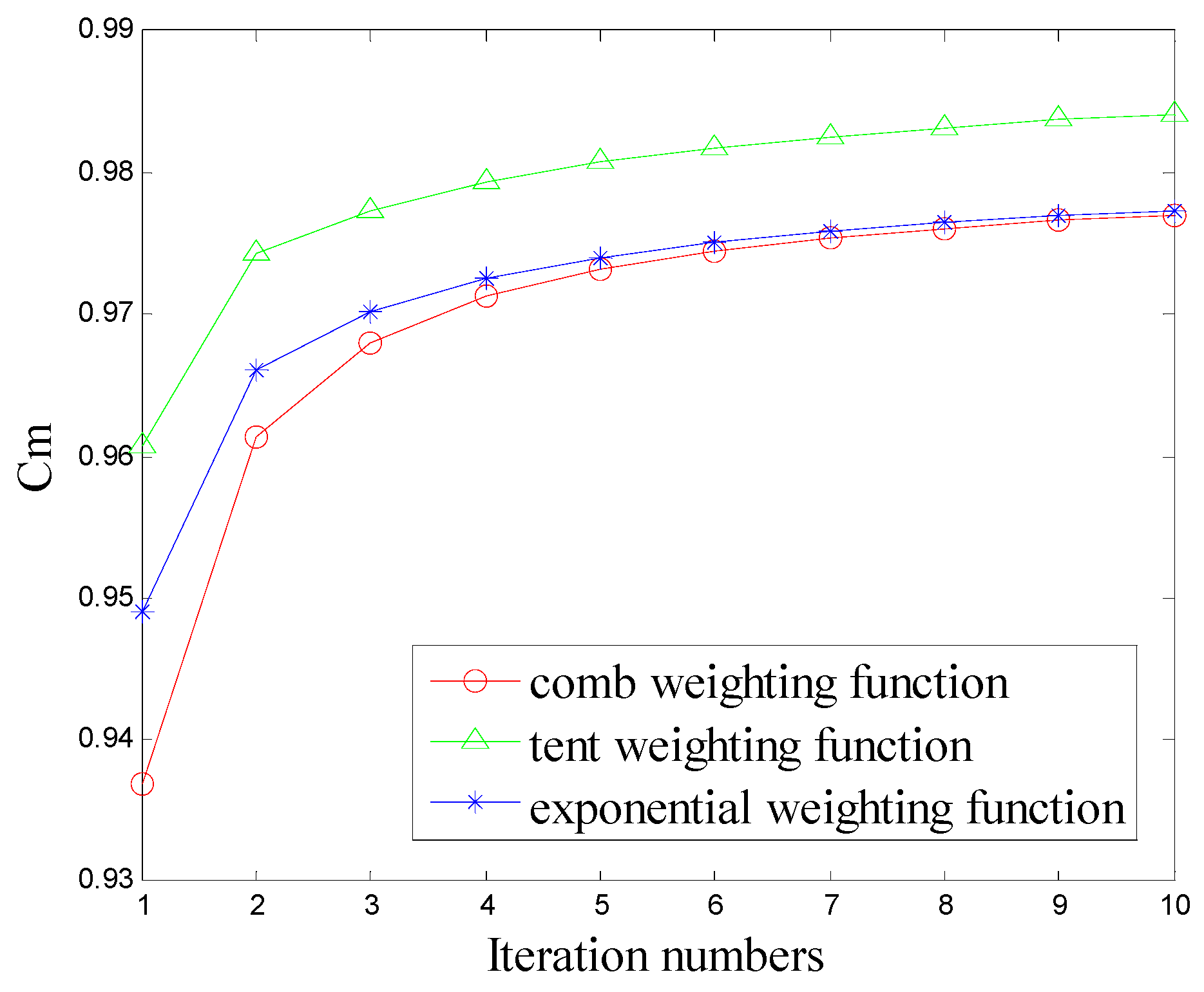
Figure 3.
Mean square error (MSE) values along with iteration.
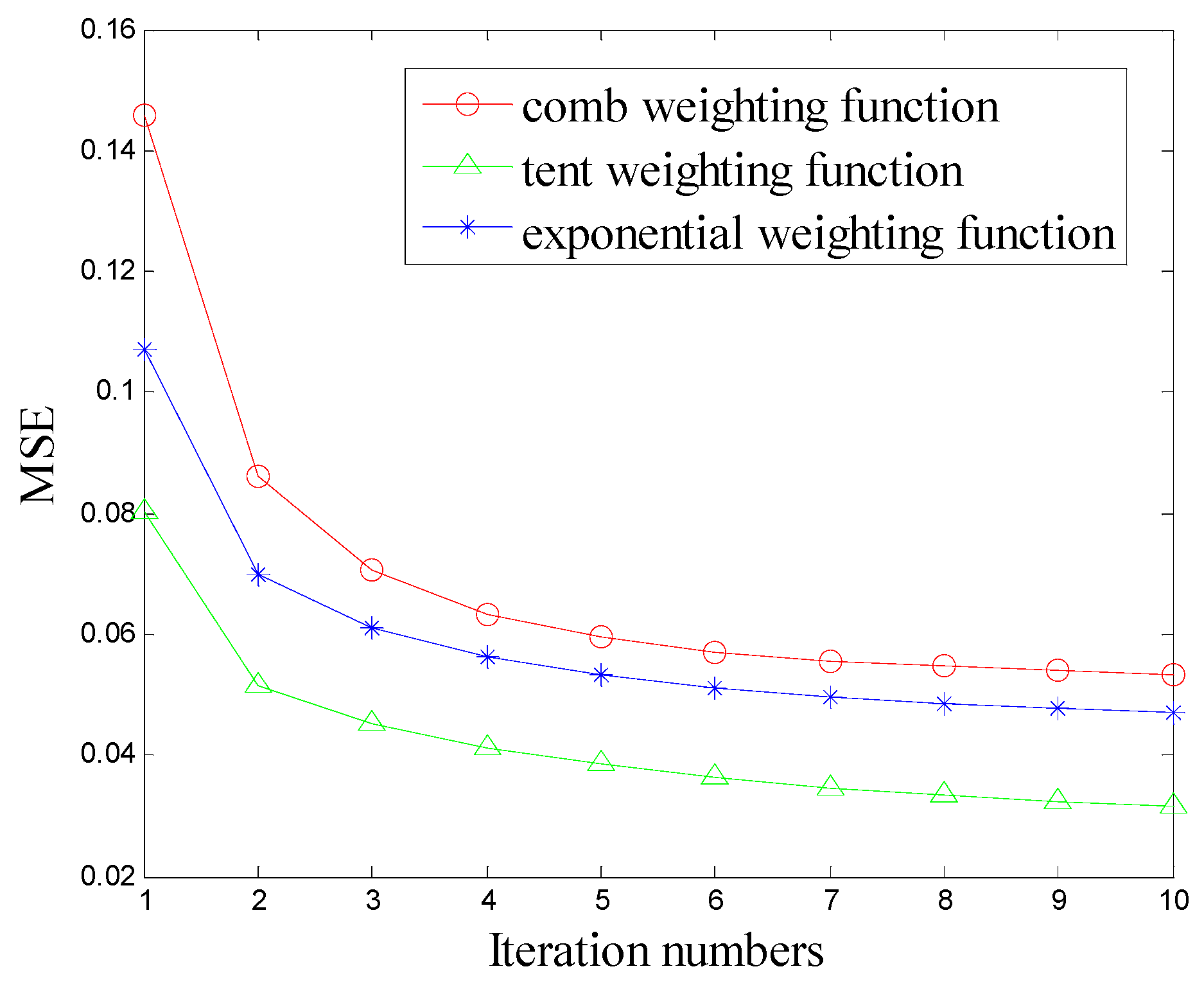
Figure 4.
SNR values along with iterations.

Figure 5.
Cm values along with iterations.

Figure 6.
MSE values along with iterations.
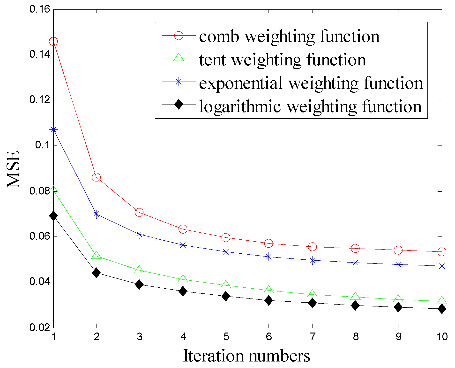
Figure 7.
The proposed method based on smooth local subspace projection and permutation entropy (PE).
Figure 7.
The proposed method based on smooth local subspace projection and permutation entropy (PE).
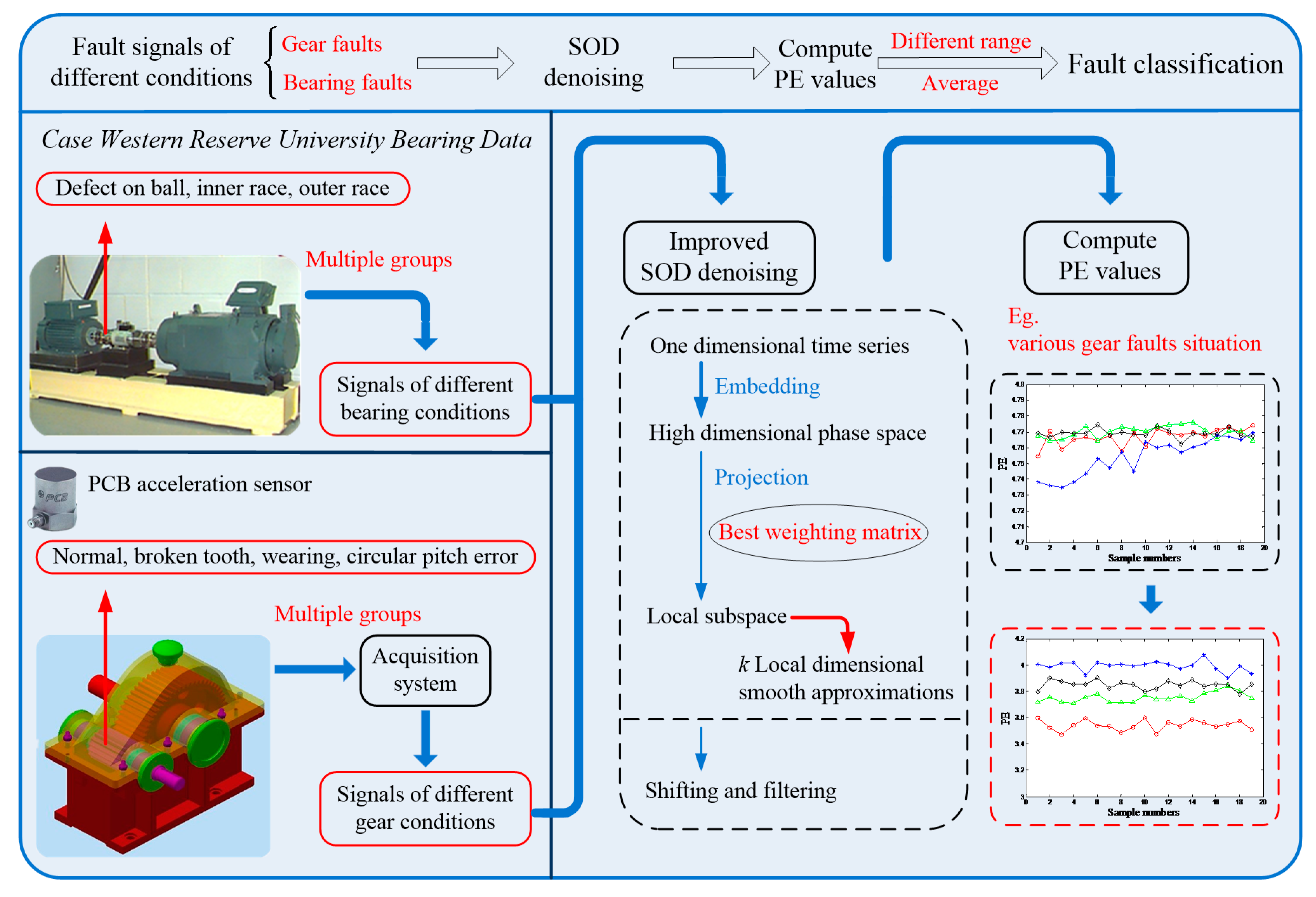
Figure 8.
of Lorenz signal.

Figure 9.
of Lorenz signal with noises.

Figure 10.
of denoised Lorenz signal with noises.
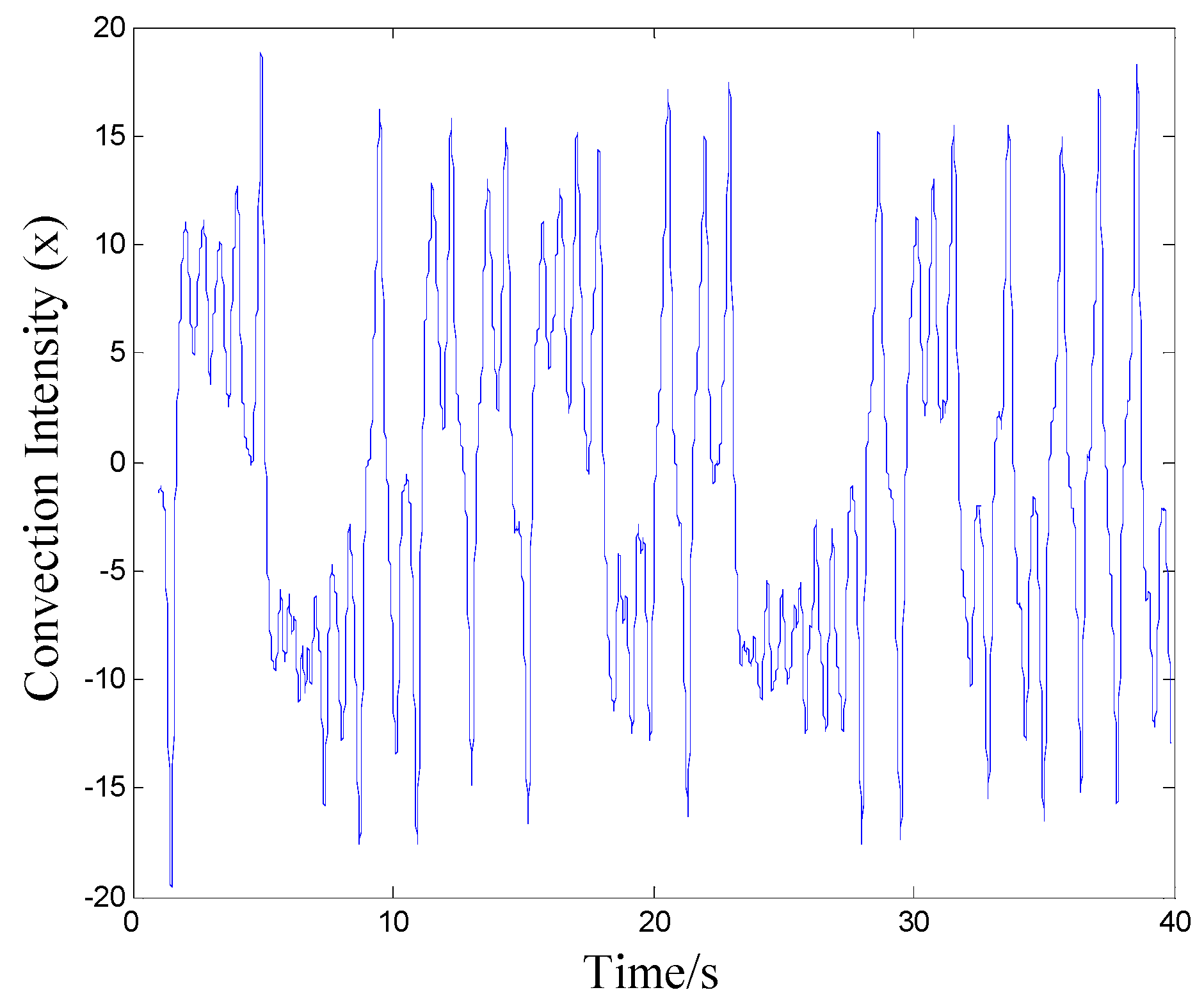
Figure 11.
The original signal, superimposed noises signal, and 7 times iteration denoised signal.

Figure 12.
SNR values along with iterations.

Figure 13.
Cm values along with iterations.
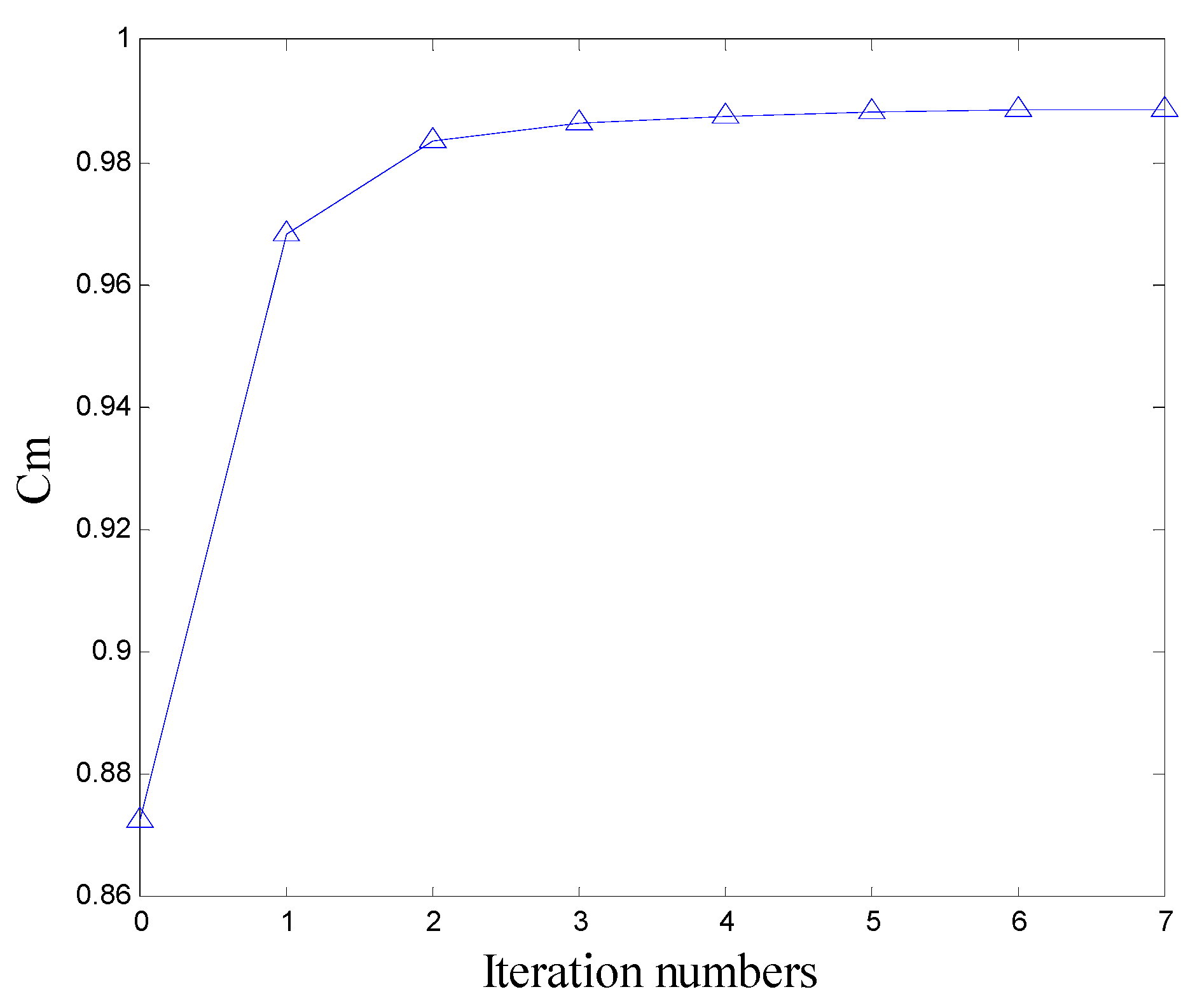
Figure 14.
MSE values along with iterations.
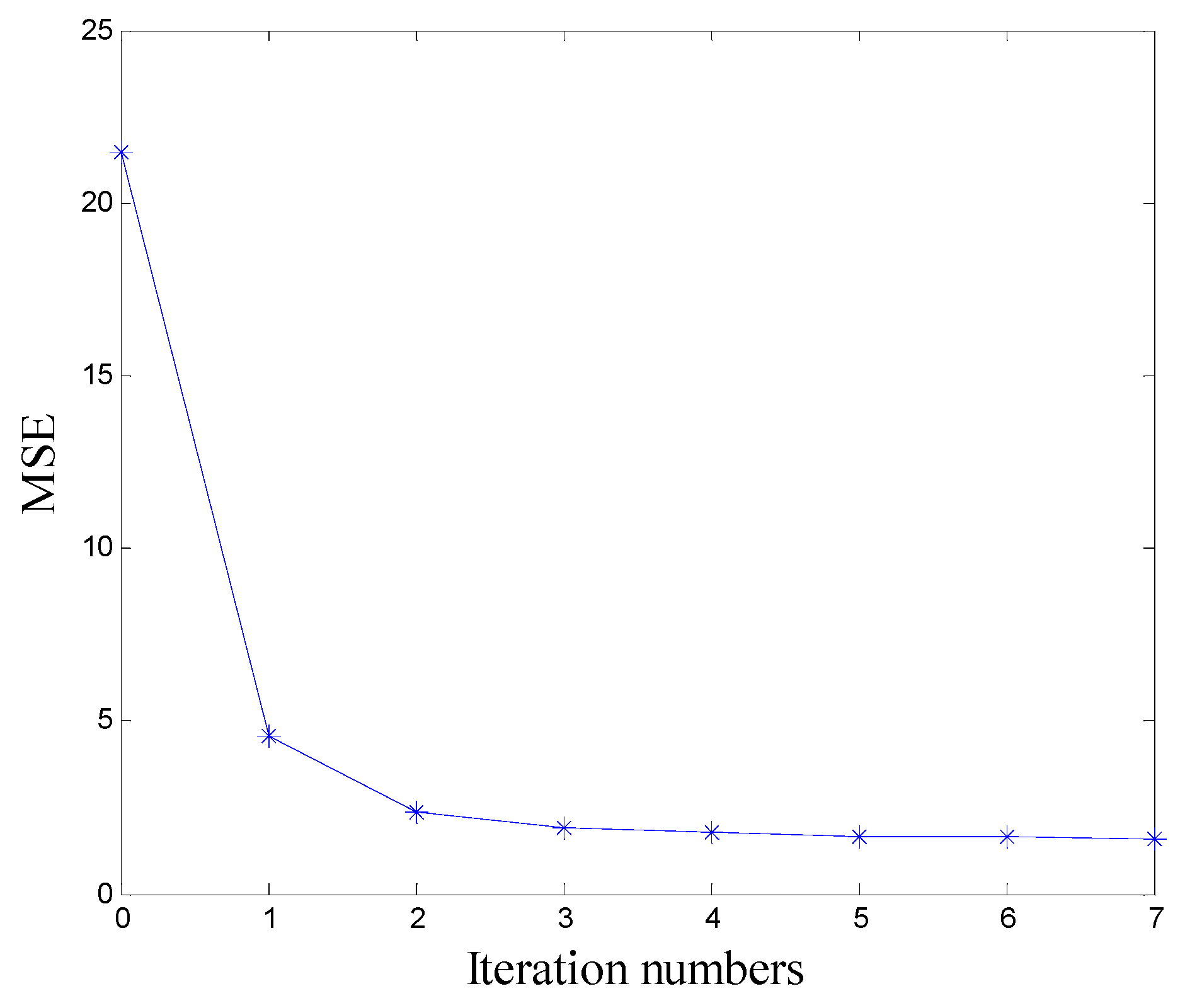
Figure 15.
Time domain plot of FM signal.
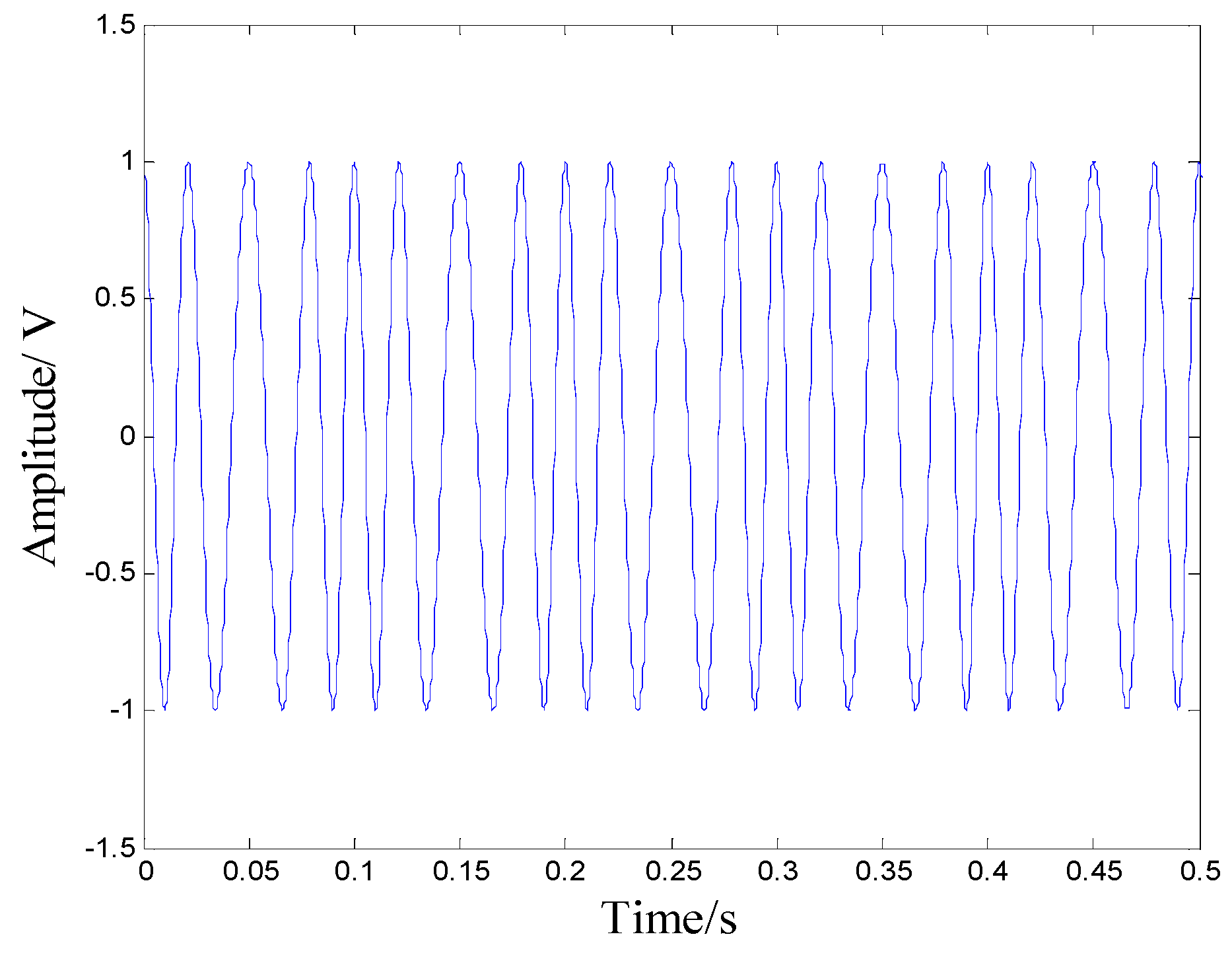
Figure 16.
Time domain plot of noisy signal.
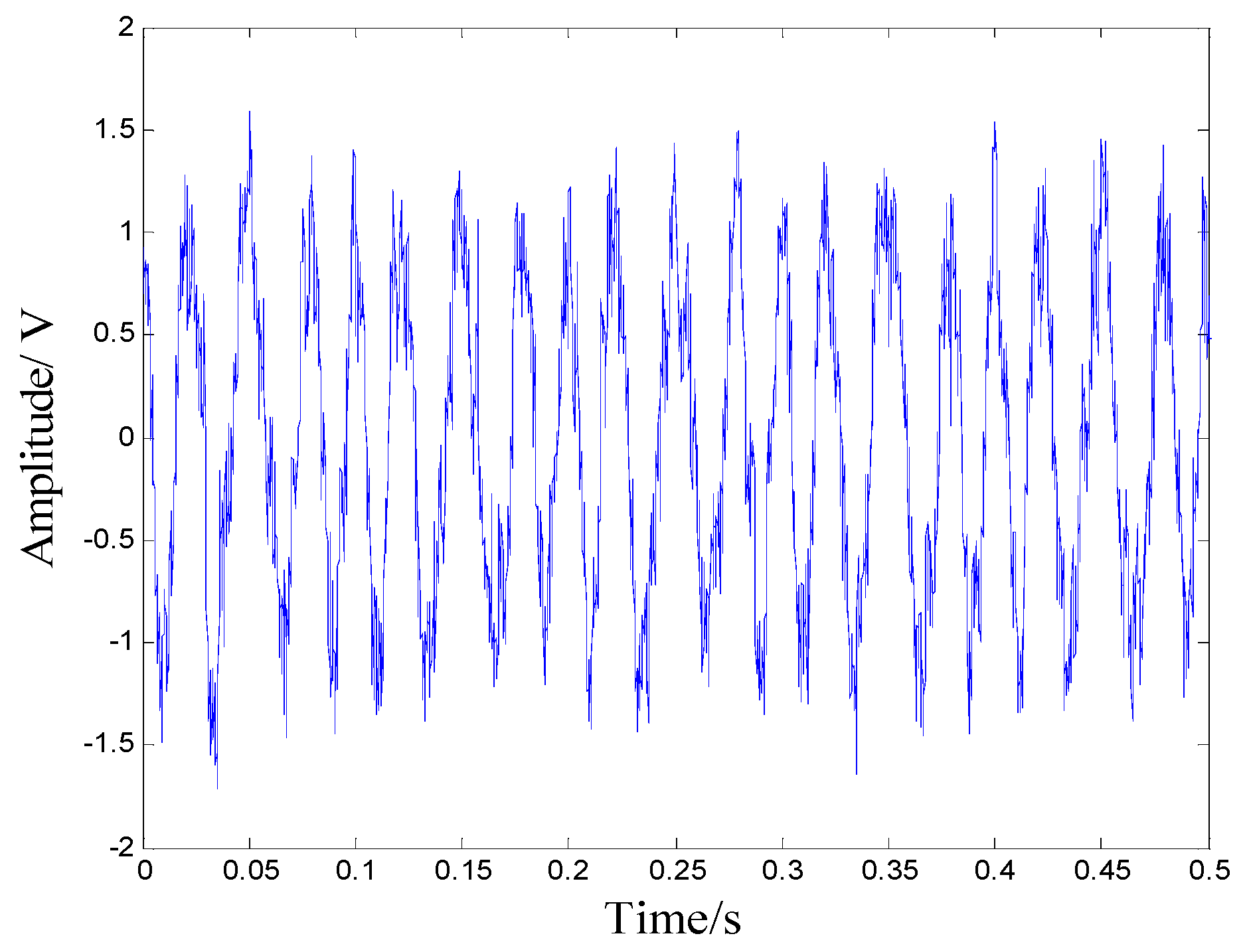
Figure 17.
Time domain plot of denoised FM signal with noises.

Figure 18.
SNR values along with iterations.
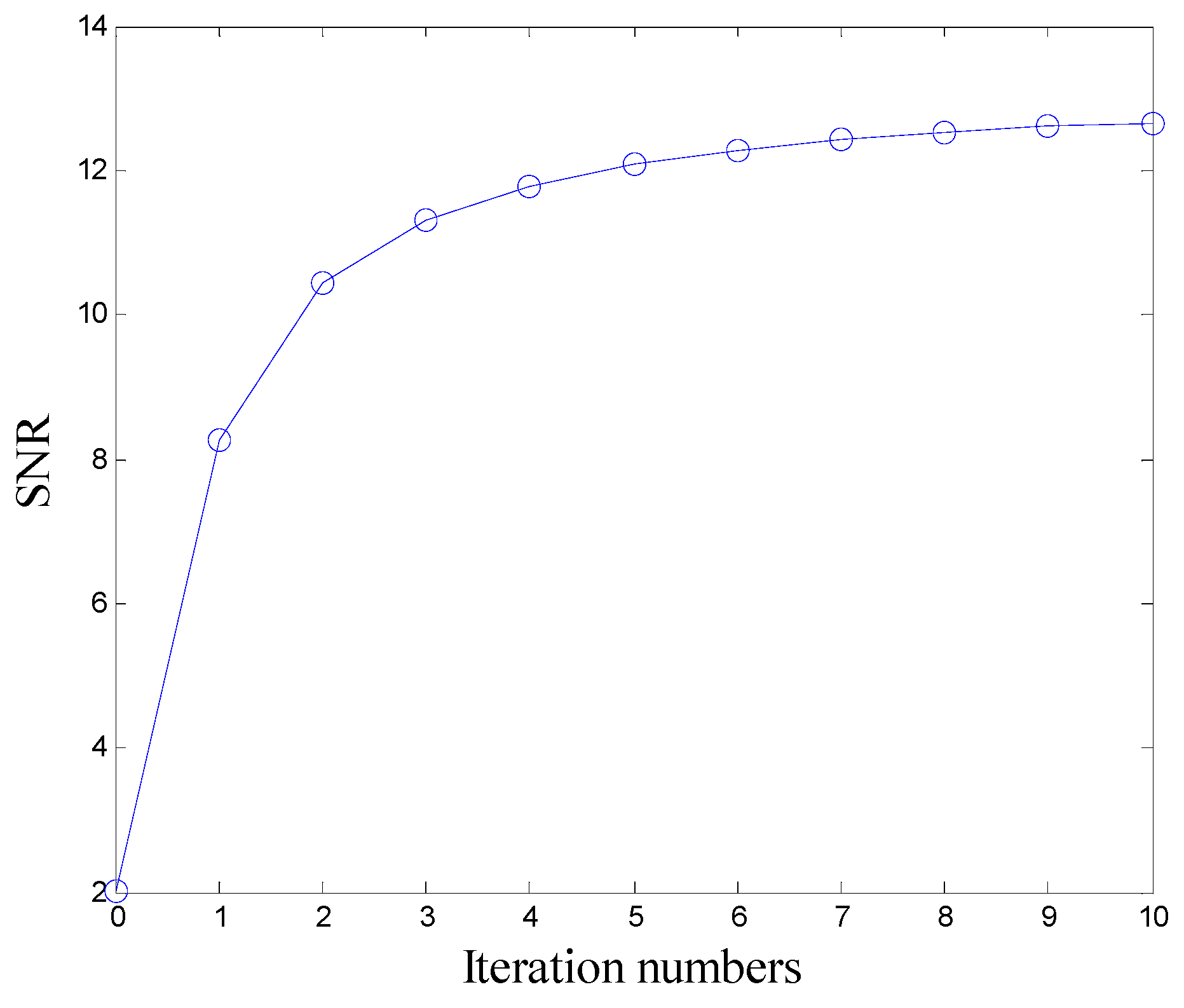
Figure 19.
Cm values along with iterations.
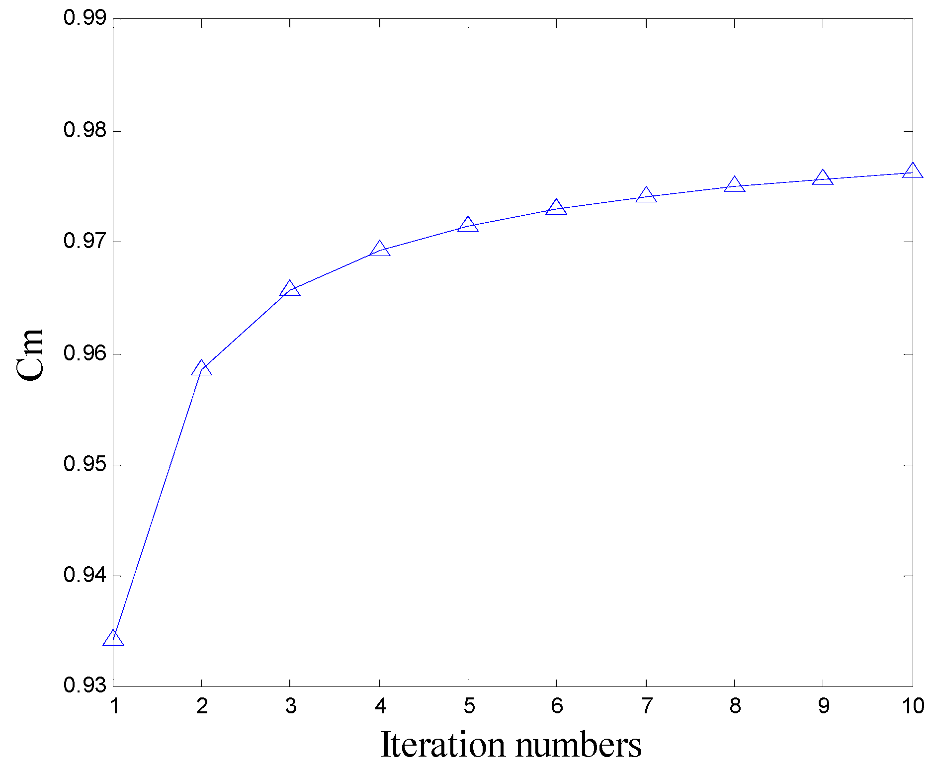
Figure 20.
MSE values along with iterations.
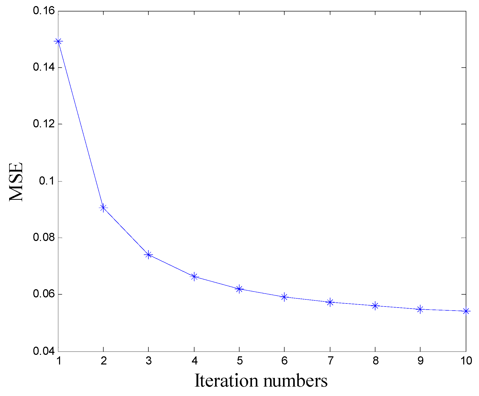
Figure 21.
Time domain plot of noisy FM signal.

Figure 22.
PE values of noisy FM signal along with time.
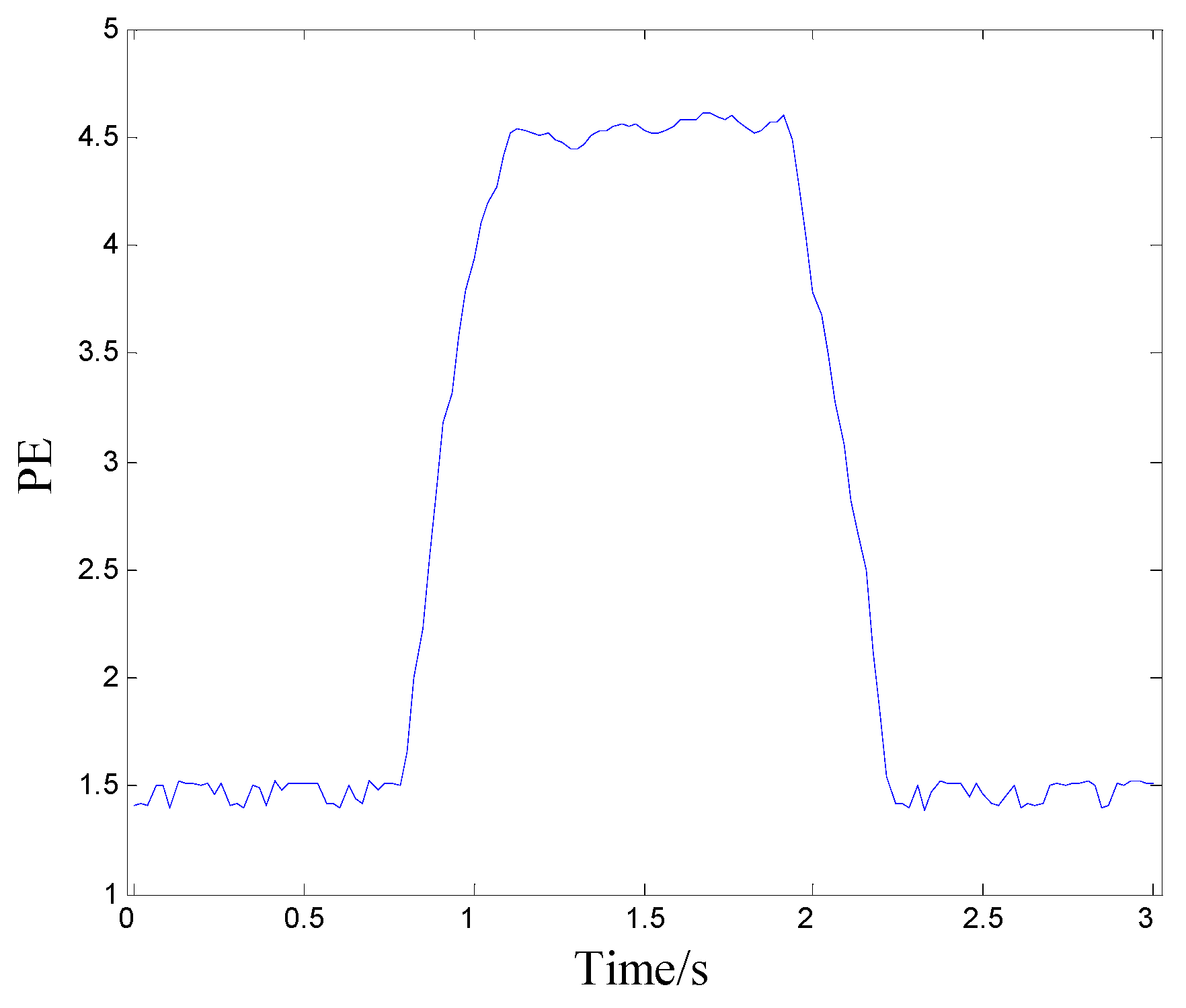
Figure 23.
The schematic diagram and a picture of the device.
1, 3-Hp motor, 2-Torque transducer and encoder.
Figure 24.
The time domain plot of ball defect.

Figure 25.
The time domain plot of inner race defect.
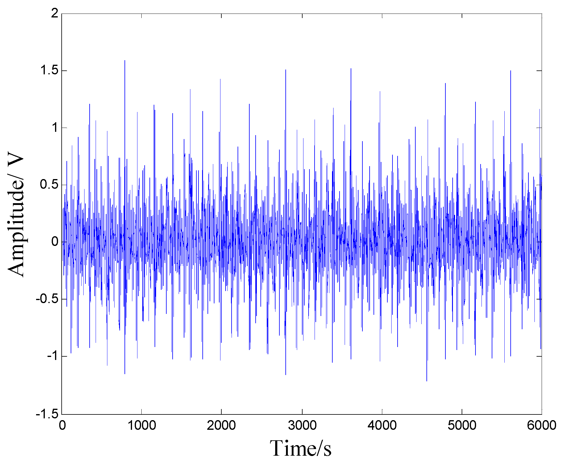
Figure 26.
The time domain plot of outer race defect.
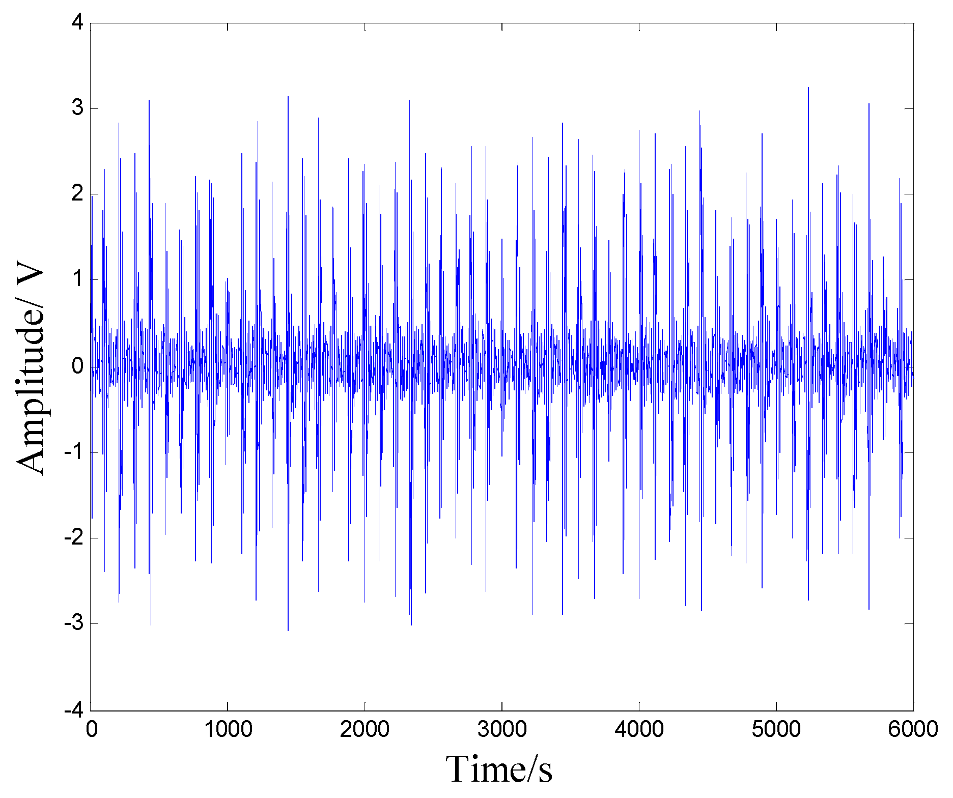
Figure 27.
The permutation entropies of original signals.
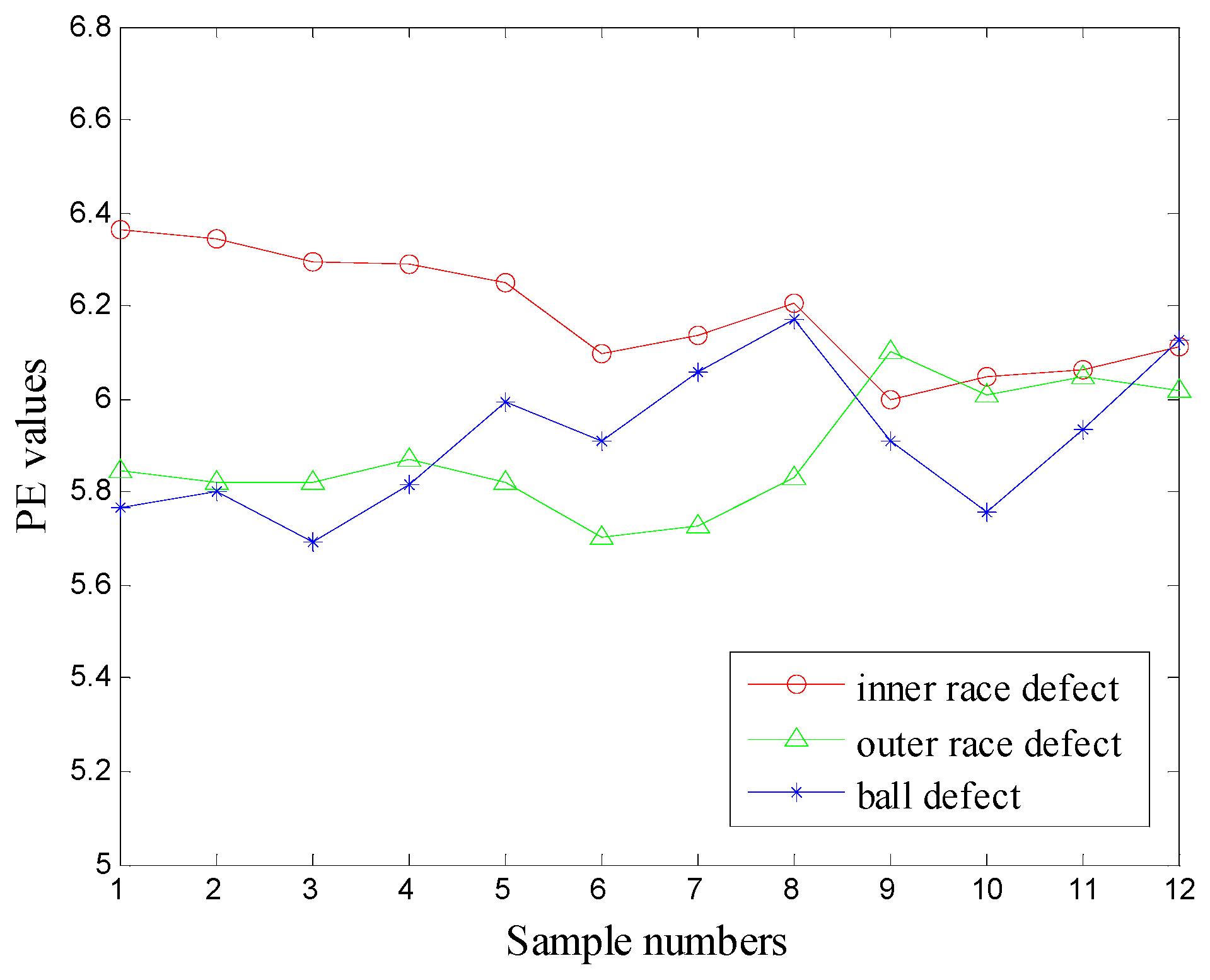
Figure 28.
The permutation entropies of the proposed approach.
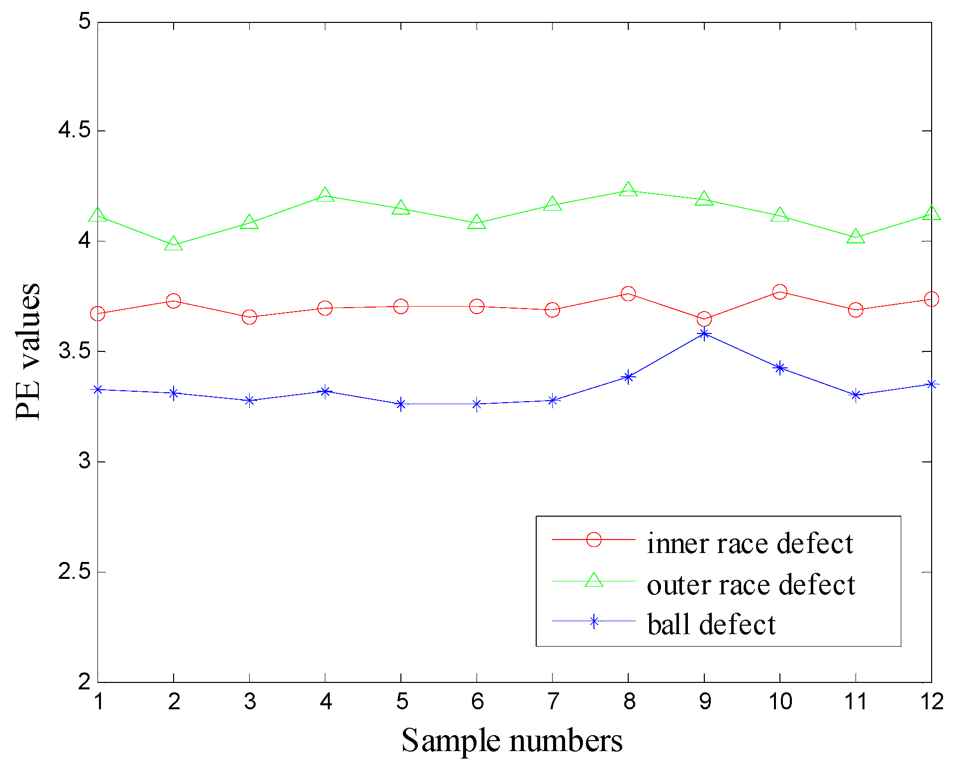
Figure 29.
The schematic diagram and a picture of the experimental apparatus.
1- Magnetic powder brake, 2-Single stage gear transmission, 3- Variable speed drive
Figure 30.
The time domain plot of normal gear.
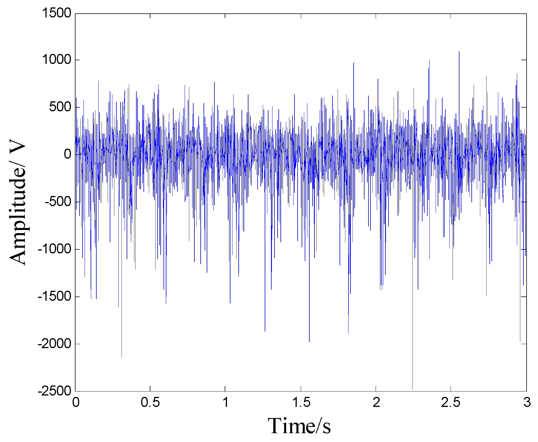
Figure 31.
The time domain plot of broken gear.
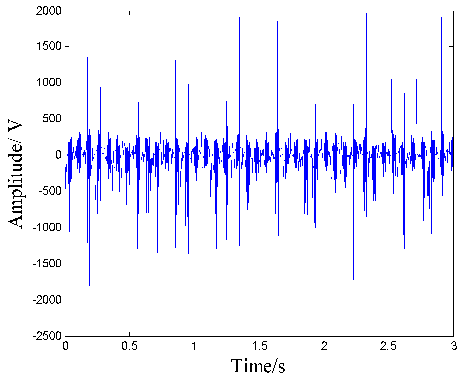
Figure 32.
The time domain plot of wearing gear.

Figure 33.
The time domain plot of circular pitch error gear.
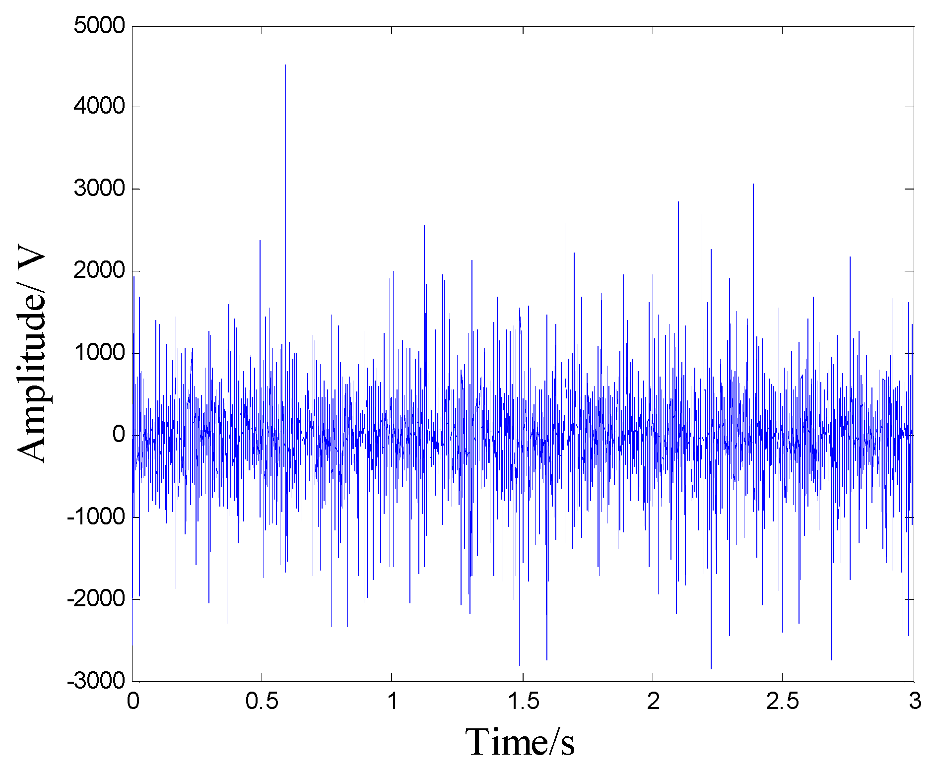
Figure 34.
The permutation entropies of original signals.

Figure 35.
The permutation entropies of the proposed approach.

Table 1.
The main steps of the smooth local subspace projection method.
| (1) Embedding of delay coordinates |
|
(2) SOD processing
|
(3) Shifting and repeating
|
Table 2.
The denoising indicators with different noise levels before and after denoising.
| SNR of Added Noise | SNR | Cm | MSE | |||
|---|---|---|---|---|---|---|
| Before | After | Before | After | Before | After | |
| −1 | −1 | 7.216 | 0.681 | 0.718 | 0.289 | 0.179 |
| −0.1 | −0.1 | 9.725 | 0.750 | 0.807 | 0.243 | 0.127 |
| 1 | 1 | 11.645 | 0.837 | 0.894 | 0.189 | 0.071 |
| 2 | 2 | 12.730 | 0.934 | 0.971 | 0.145 | 0.047 |
Table 3.
Rolling element bearing parameters.
| Rolling Element Bearing Parameters of 6205-2RS JEM SKF (Diameter/mm) | |||||
|---|---|---|---|---|---|
| Ball number n | Contact angle α | Ball diameter dr | Outside diameter d2 | Inside diameter d1 | Pitch diameter Dw |
| 9 | 0 | 7.9 | 52 | 25 | 46.4 |
© 2019 by the authors. Licensee MDPI, Basel, Switzerland. This article is an open access article distributed under the terms and conditions of the Creative Commons Attribution (CC BY) license (http://creativecommons.org/licenses/by/4.0/).
Share and Cite
MDPI and ACS Style
Xiao, L.; Lv, Y.; Fu, G. Fault Classification of Rotary Machinery Based on Smooth Local Subspace Projection Method and Permutation Entropy. Appl. Sci. 2019, 9, 2102. https://doi.org/10.3390/app9102102
AMA Style
Xiao L, Lv Y, Fu G. Fault Classification of Rotary Machinery Based on Smooth Local Subspace Projection Method and Permutation Entropy. Applied Sciences. 2019; 9(10):2102. https://doi.org/10.3390/app9102102
Chicago/Turabian StyleXiao, Lingjun, Yong Lv, and Guozi Fu. 2019. "Fault Classification of Rotary Machinery Based on Smooth Local Subspace Projection Method and Permutation Entropy" Applied Sciences 9, no. 10: 2102. https://doi.org/10.3390/app9102102
Note that from the first issue of 2016, this journal uses article numbers instead of page numbers. See further details here.