Study of Heat and Mass Transfer in Electroosmotic Flow of Third Order Fluid through Peristaltic Microchannels

1
Department of Mathematics, Comsats University Islamabad, Tarlai Kalan Park Road, Islamabad 44000, Pakistan
2
Division of Computational Mathematics and Engineering, Institute for Computational Science, Ton Duc Thang University, Ho Chi Minh City 700000, Vietnam
3
Faculty of Mathematics and Statistics, Ton Duc Thang University, Ho Chi Minh City 700000, Vietnam
*
Author to whom correspondence should be addressed.
Appl. Sci. 2019, 9(10), 2164; https://doi.org/10.3390/app9102164
Submission received: 18 April 2019
/
Revised: 8 May 2019
/
Accepted: 10 May 2019
/
Published: 27 May 2019
(This article belongs to the Special Issue Heat and Mass Transfer: Fundamentals and Applications in Thermal Energy)
Abstract
:An analysis is carried out to evaluate the effects of heat and mass transfer in an electro-osmotic flow of third order fluid via peristaltic pumping. Solutions are derived for small wave number and Peclet number. The emerging non-linear mathematical model is solved analytically and compared numerically by the built-in scheme of working software. The table is inserted for shear stress distribution and a graph for comparison of solution techniques and accuracy of obtained results. The effects of various parameters of interest on pumping, trapping, temperature, heat transfer coefficient, and concentration distribution have been studied graphically. Electro-osmotic exchange of energy and mass has a role in reservoir engineering, chemical industry, and in micro-fabrication technologies.
1. Introduction
In the past few decades, electroosmosis has found rich applications. The first microfluidic devices were developed in the 1980s with the name Micro-Electro-Mechanical Systems (MEMS). These devices have broad application prospects in a variety of fields including biological and medical-related industries, where microfluidic devices are referred to as Lab-on-chip (LOC) devices. LOC can be used in many applications including clinical diagnostics, and biological or chemical contamination. Today, the need for the reliable, fast and well-organized performance of the microfluidic system has created a rigorous demand for small, easy-to-operate and cheap systematic apparatus for drug delivery and DNA analysis.
Microfluidic devices typically use electroosmosis to pump fluid into the entire device. Electroosmosis describes the flow of electrolyte through a channel having a charged boundary due to an applied voltage. Electro-osmosis occurs in many biological, medical and industrial processes such as porous membranes, tubule/canalicular flow, botanical processes, fluid dialysis, transport in human skin and separation techniques. Haung et al. [1] explained the Electroosmotic flow (EOF) in capillaries by monitoring method. Gravesen et al. [2] reviewed the detailed applications of microfluidics. Haswell [3] scrutinized the developmental features of micro-flows on EOF basis. Patankar and Hu [4] predicted the simulation of EOF. Also, Kang et al. [5] examined the EOF in the annulus of capillaries.
The dynamics of peristaltic flow are triggered by its emergence of physiology (intestines, ureters, esophagus, bile ducts, catheters, granules, etc.) and industry (blood pumps, transport of corrosive liquids and hygienic fluid transport). Most of the research on this topic has been conducted on Newtonian fluids. Non-Newtonian fluids cannot be elucidated by a single constitutive relation. Hence, several constitutive relations of these fluids have been proposed. The impact of viscosity in peristalsis for third-grade fluid was explored by Hayat and Abbasi [6]. Noreen [7] proposed the physiological motion of the third order fluid with a magnetic field and mixed convection. Moreover, Noreen [8] considered the peristaltic motion of MHD couple-stress fluid. Prakash et al. [9] worked on peristaltically induced third-grade fluid via the asymmetric conduit. Mallick and Misra [10] discussed Erying–Powell fluid with the electromagnetic field.
Mathematical simulations of peristaltic distribution in microfluidic devices have newly attracted attention. Peristaltic motion can be controlled by adding and resisting external electric fields. One such example is the addition in peristaltic flow by electroosmosis [11]. Tang et al. [12] explored the electroosmosis in the power-law fluid. Hadigol et al. [13] considered the microscopic mixing characteristics of the power-law fluid in electroosmosis. Yavari et al. [14] demonstrated an increase in EOF temperature of bio-fluids (non-Newtonian) via microchannel. Furthermore, Bandopadhyay et al. [15] studied electroosmosis and peristalsis in microchannels. Likewise, Jiang et al. [16] investigated the effect of electroosmosis for Oldroyd-B fluid and wall slip. Jhorar et al. [17] expounded the biomechanical transfer through asymmetric microconduit. Similarly, Tripathi et al. [18] inspected the microvascular blood transport via EOF. Francesko et al. [19] observed the progress of LOC and microfluidics in detail. Javavel et al. [20] illustrated the EOF of pseudoplastic nano liquids through peristaltic pumping. However, the above studies did not examine the electroosmotic effects in peristaltically flowing third order fluid.
Heat transfer in microfluidic devices is of great importance in cancerous tissues destruction, portable kits for diseases diagnostics, the examination of dilution techniques in blood flow and the micro-fabrication technologies. Sadeghi et al. [21] examined the effect of heat exchange in EOF for viscoelastic fluids. Babaie et al. [22] noticed the impact of heat flow for Power-law fluid in the microchannel. Further, Chen et al. [23] analyzed heat exchange for Non-Newtonian fluid suspension in the microchannel. Thermal exchange in blood through capillaries was incorporated by Sinha and Shit [24]. Shit et al. [25] also showed the EOF for heat exchange and MHD. Moreover, in medical operations, it is considered that the wavy walls in electroosmotic flow increase the mass transfer. Therefore, Bhatti et al. [26] described the heat and mass transmission through EDL effects. Also, Reddy et al. [27] revealed the heat transport in peristaltic pumping for Casson fluid through the microchannel. Peristaltic pumping with EDL was studied by Yadav et al. [28]. Narla et al. [29] examined the effect of heat in EOF through time. Moreover, Yang et al. [30] also depicted the transportation of heat in magneto-hydrodynamic EOF.
To our knowledge, there is currently no report on heat and mass transfer in EOF of third-order fluid altered by peristalsis. The present study fills the gap. The main purpose of the present investigation is to analyze the effect of heat transfer and mass transfer for EOF of a third order fluid with viscous dissipation in a microchannel. Note, third order fluid has outstanding significance for shear thickening and shear thinning properties. This investigation has been carried out by using lubrication approximation and Debye Hückel linearization. The non-linear governing equations are solved through perturbation method. Pressure rise and heat transfer coefficient at channel walls have been calculated numerically. Finally, the graphical results for physical quantities are drawn and discussed in detail.
2. Mathematical Model
2.1. Flow Analysis
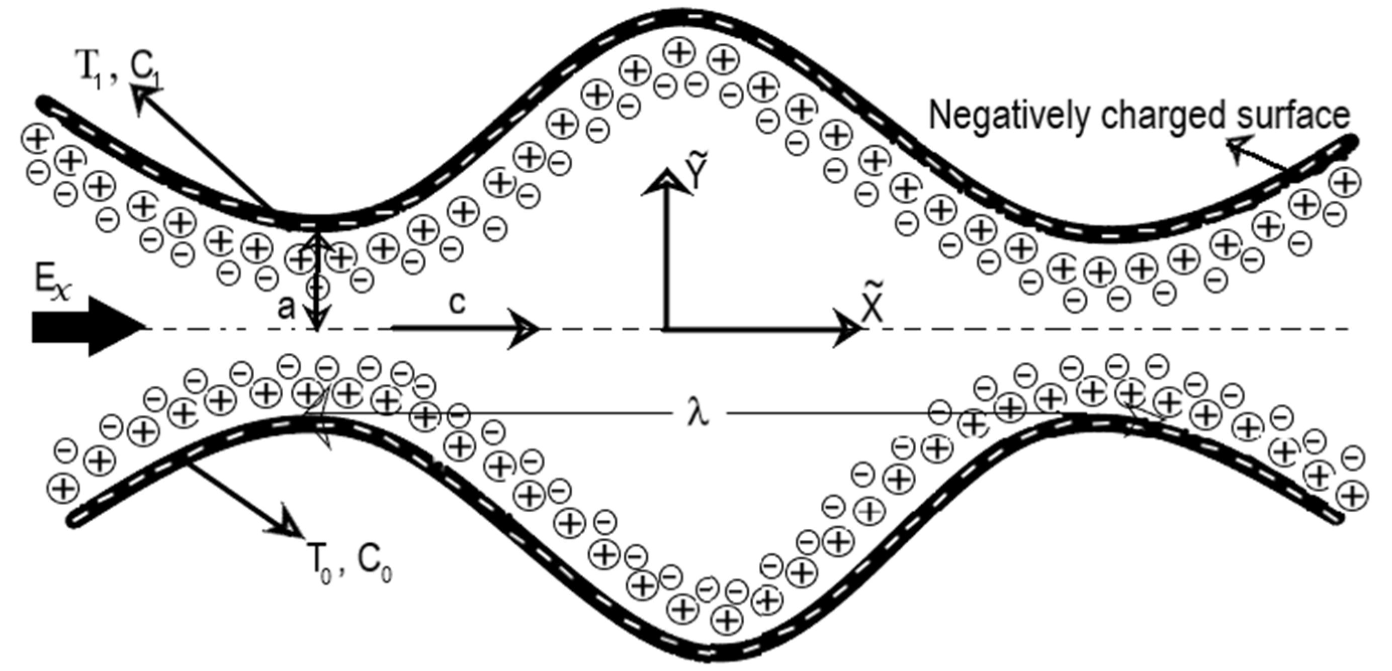
Consider 2D electroosmotic flow (EOF) of third order fluid in a microfluidic channel having a width , presented in Figure 1. A peristaltic wave at velocity propagates along the microchannel wall. The temperature and concentration fields of the lower channel wall are maintained at and whereas upper at and , respectively.
Mathematically, microchannel geometry is expressed as:
Here and are the axial coordinate, channel’s half width, wave amplitude, wave speed, wavelength and time respectively.
2.2. Governing Equations
In the laboratory frame, governing equations for flow of third order fluid in electrohydrodynamic (EHD) environment are [17]:
Continuity Equation:
Equation of motion:
Energy equation with viscous dissipation [9]:
Concentration equation:
Here is the velocity along direction, along direction, is electrical charge density, is pressure, is density of fluid, is axial electric field, is the specific heat, is thermal conductivity, is ratio of thermal diffusion, is mass diffusivity coefficient, is average temperature, is temperature and is concentration field, which are dimensional.
Stress tensor for fluid [6] is defined as
where and are the material constants. Similarly, Revilin Erickson tensors are
The thermodynamic analysis of the model [7] shows that if all the fluid motion is thermodynamically compatible, then these motions must satisfy the Clausius–Duhem inequality. Moreover, it is also supposed that the specific Helmholtz free energy be minimal in equilibrium, then
In the present investigation, we assume that fluid is thermodynamically compatible, so Equation (7) reduces to the form
2.3. Electrohydrodynamics (EHD)
The Poisson equation [11] in a microchannel is described as:
Here and represents total charge density, dielectric permittivity, and electric potential.
2.4. Potential Distribution
The net charge density follows the Boltzmann distribution [12], given as
here the anions and cat-ions are defined through of the Boltzmann Equation:
where represents bulk concentration, the charge balance, the Boltzmann constant, the electronic charge and is the average temperature.
Applying Debye-Hckel linearization approxiamtion [12], Equation (11) becomes
Here is the electroosmotic parameter. The analytical solution of above Equation (14) subject to boundary conditions at and at is obtained as;
2.5. Non-Dimensionlization, Lubrication Approach and Boundary Conditions
In the stationary frame , the motion is unsteady due to the moving boundary. But, if viewed in a moving frame , it can be considered as steady due to static boundary. Therefore, the translational transformation between two frames is [7]:
The above transformations is used in Equations (2)–(6) and then introducing the non-dimensional variables:
Here, and are the axial and transverse coordinate, is electroosmotic parameter, is dimensionless pressure, is Debye length, is peristaltic wave number, is dimensionless volume flow rate, is dimensionless temperature, is dimensionless concentration, is Helmholtz–Smoluchowski velocity, is non-dimensional stream function, is ionic Peclet number, is Brinkman, is Reynolds number, is Prandtl, is Deborah number, is amplitude ratio, is non-dimensional shear stress, is non-dimensional Soret number, is Schmidt number and is Eckert number.
The relation of velocity and stream function is defined as
After introducing Equations (17) and (18), Equation (2) is satisfied identically and Equations (3)–(6) becomes
Now subject to long-wavelength assumption [10] on Equations (19)–(22), ignoring higher powers of , we get;
where .
Eliminating pressure from Equations (23) and (24), we get
The dimensionless boundary conditions are:
here is dimensionless mean flow rate in moving frame and is dimensionless mean flow rate in fixed frame. Furthermore, in the moving frame is connected to the in the fixed frame as:
here .
3. Solution Methodology
3.1. Series Solutions
The governing differential system given in Equations (23)–(27) subject to boundary conditions (28,29) consists of highly non-linear and coupled equations. Exact solution of the governing system of equations is impossible. Therefore, analytical solution of the system is presented through the perturbation technique by taking Deborah number as a perturbation parameter. So, we expand , , . and as in [8]:
3.2. Zero Order System
3.3. First Order System
The solution for zero and first order system is defined in the appendix. By substituting the zero and first order solution in the Equations (32)–(35) we get the final first order solution for , , and .
The dimensionless pressure rises per wavelength is as follows:
The heat transfer coefficient is defined as:
The shear stress at the wall is defined as
4. Computational Discussion of Results
This section deals with the impacts of different parameters (i.e., Deborah number , electroosmotic parameter , Helmholtz–Smoluchowski/maximum electroosmotic velocity , Brinkman number , volume flow rate , Soret number and Schmidt number ) on the pressure rise , pressure gradient , velocity distribution , temperature distribution , concentration distribution , heat transfer coefficient and streamlines . Figure 2, Figure 3, Figure 4, Figure 5, Figure 6, Figure 7, Figure 8, Figure 9, Figure 10 and Figure 11 are plotted to serve the purpose.
4.1. Comparative Analysis
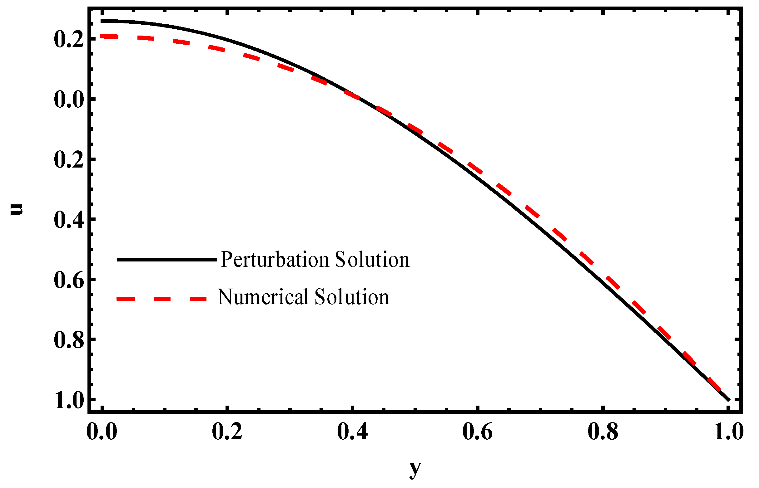
Figure 2 reveals the overlapping comparison between the analytical and numerical solution of velocity. Note that the analytical solution is obtained through perturbation technique and numerical solution is from built-in scheme NDsolve of working software. It is concluded that our results through perturbation (i.e., truncated up to first order of third-order fluid parameter) are in good agreement with the numerical scheme.
4.2. Flow Characteristics
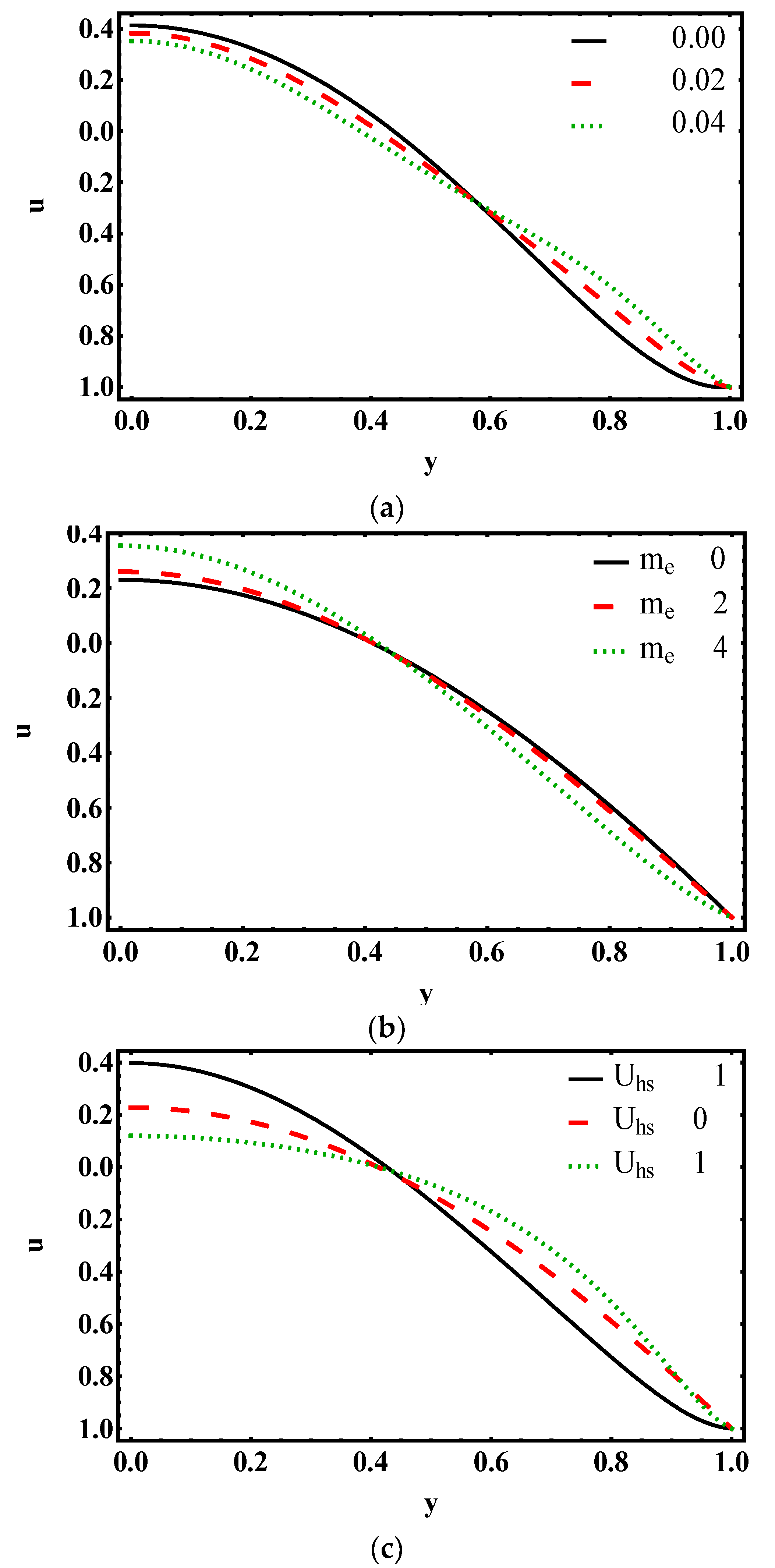
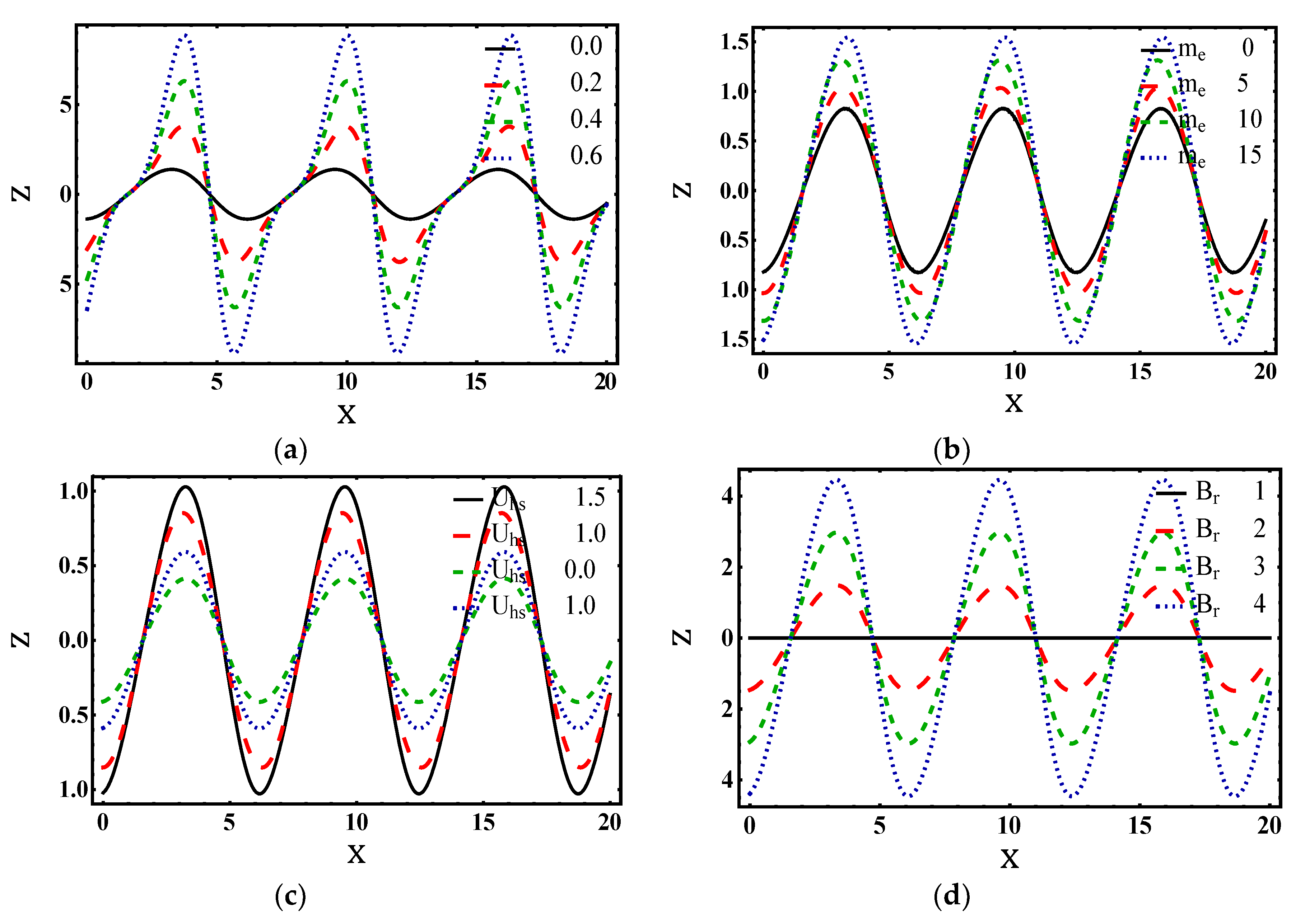
The axial velocity deserves to provide the main features of flow behavior in the microchannel for microfluidic applications. Figure 3a–c is portrayed to inspect the evolutions in the velocity profile across the microchannel for various values of Deborah number , electroosmotic parameter and maximum electroosmotic velocity . Figure 3a shows the variation of axial velocity for various values of . It is demonstrated that the magnitude of velocity decreases as increases at . The reason behind this trend is EDL (electric double layer). It means flow of fluid resists in the presence of EDL. But opposite behavior is witnessed near the channel wall . Figure 3b predicts that boosts the magnitude of i.e., magnitude of increases as increases at the central region of the channel and reduces near the walls of the channel. Since is the ratio of the channel height to the Debye length , it specifies that is inversely proportional to EDL. Hence, more fluid flows in the central region . Figure 3c depicts that decent as ascents in , whereas opposite movement is noticed at . As physically concludes that velocity of fluid decreases when thickness of EDL increases. Therefore, fluid flow decreases in EDL presence.
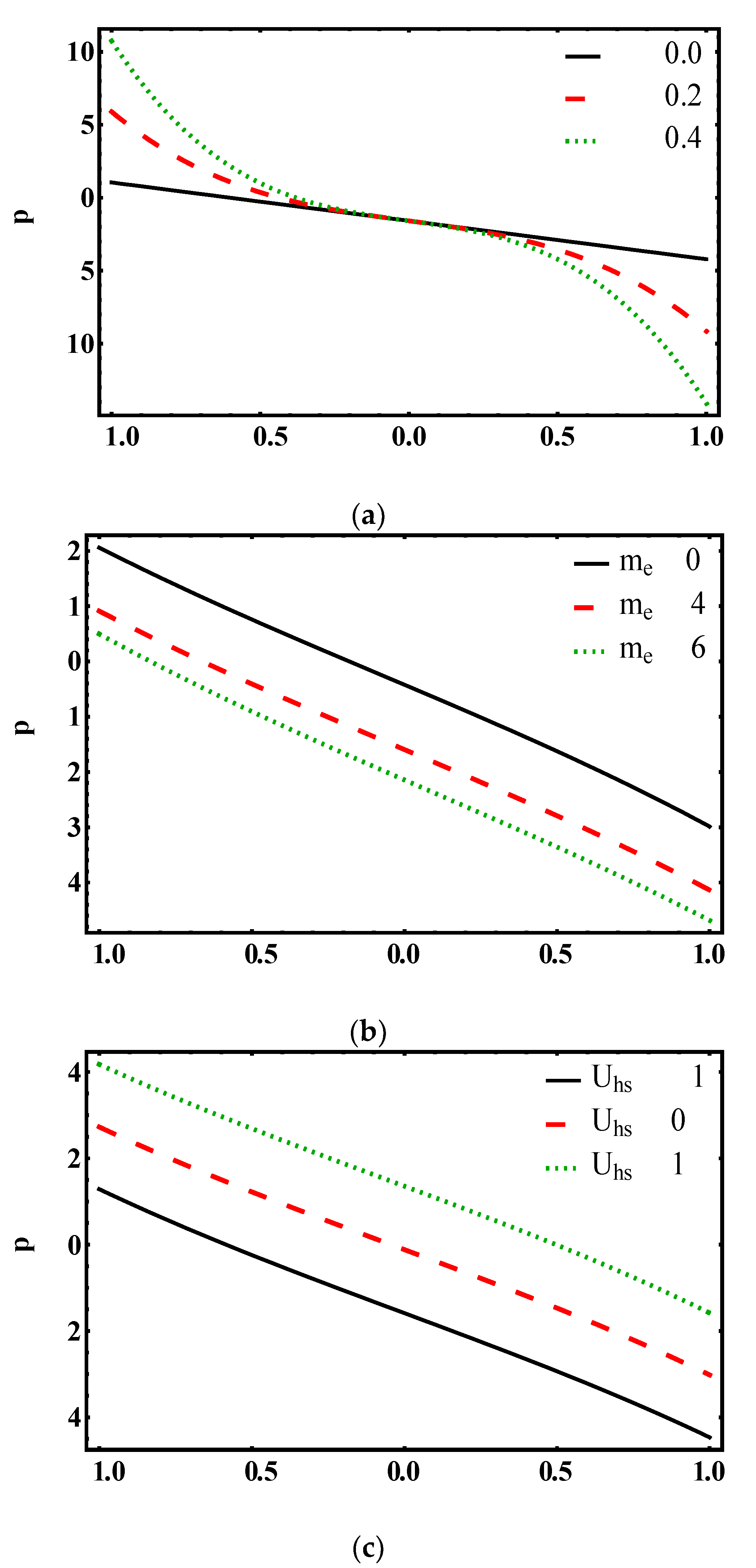
4.3. Pumping Characteristics
Peristalsis is characterized by pushing the fluid forward against the pressure rise . The characteristic of pumping can be analyzed in the form of versus shown in Figure 4a–c Pumping action divides the whole region into the four segments: pumping region (adverse pressure gradient , Positive pumping , backward/retrograde pumping (,), augmented pumping (favorable pressure gradient , Positive pumping ) and free pumping (). Figure 4a portrays the against for different values of . It is perceived that pumping increases as increases in pumping region (). But in co-pumping (), pumping decreases as increases. It means that pumping rate is high for third order fluid under parameter in comparison to viscous fluid . For free pumping (), curves coincide i.e., there is no difference between third-grade fluid and Newtonian fluid within the domain of −0.4 to 0.4. Figure 4b describes that decreases as increases. This means additional pressure is needed to drive the third-grade fluid for maximum thickness of EDL. It physically declares that formation of EDL on charged surface opposes the third-grade fluid flow. Furthermore, Figure 4c illustrates decreases as increases. Here pumping is controlled through an electric field. Note that there is a linear relationship between against because of .
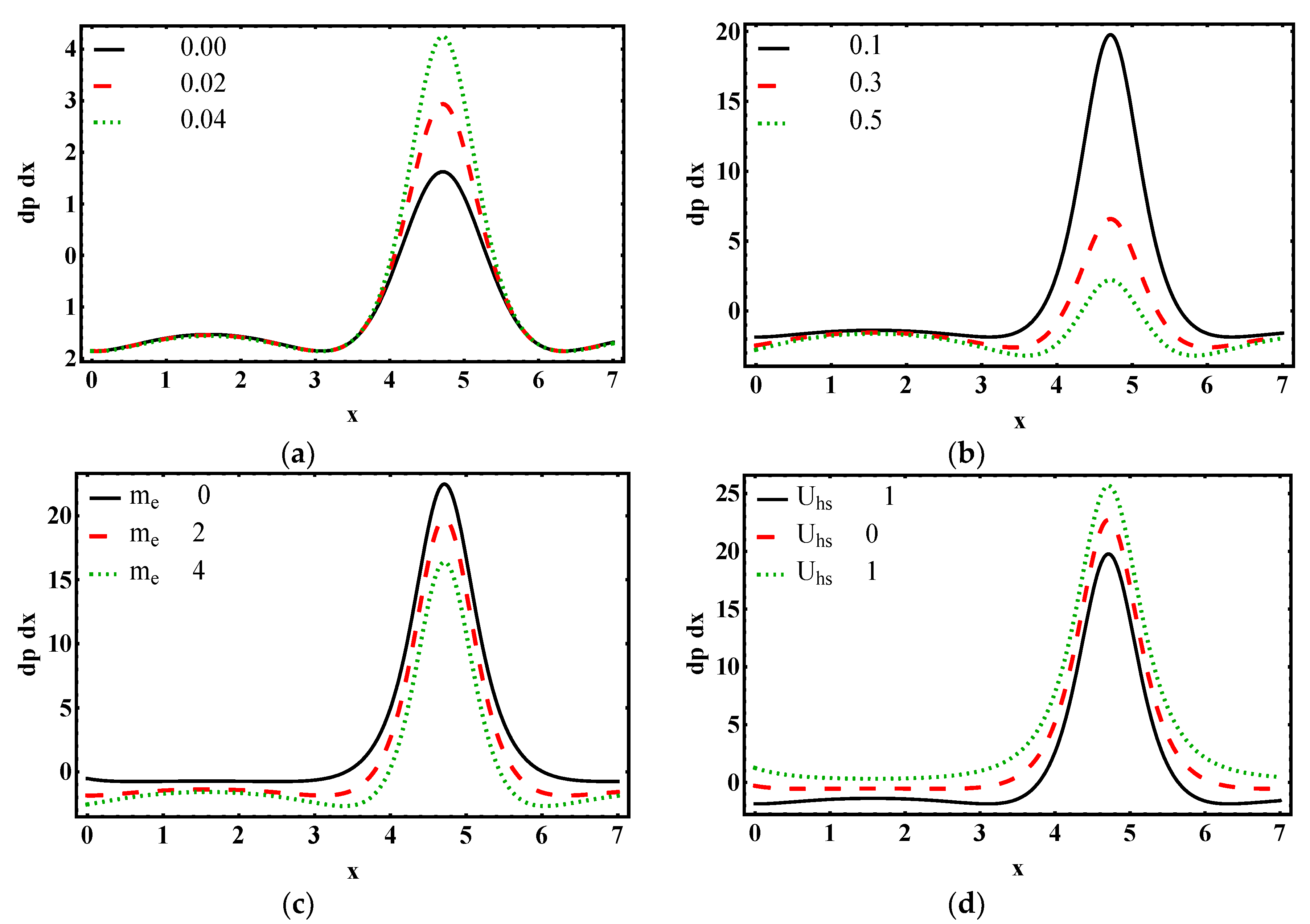
The distribution of pressure gradient is plotted through Figure 5a–d for Deborah number , electroosmotic parameter , maximum electroosmotic velocity and volume flow rate . Figure 5a portrays that by increasing the magnitude of pressure gradient increase. being a physical parameter showing the Non-Newtonian nature, one can observe pressure gradients are higher for third order in comparison to Newtonian fluids. Figure 5b illustrates that by increasing the values of . decreases. Because there is an inverse relationship between and . Figure 5c highlights that by raising the values of . decreases. It means that EDL presence in charged surface resists the flow of third grade fluid. Similarly, it is important that the characteristics of pumping can be modified by EDL mechanism and process of pumping can be systematized by thinning and thickening EDL width. Also, Figure 5d presents that the magnitude of increases as increases.
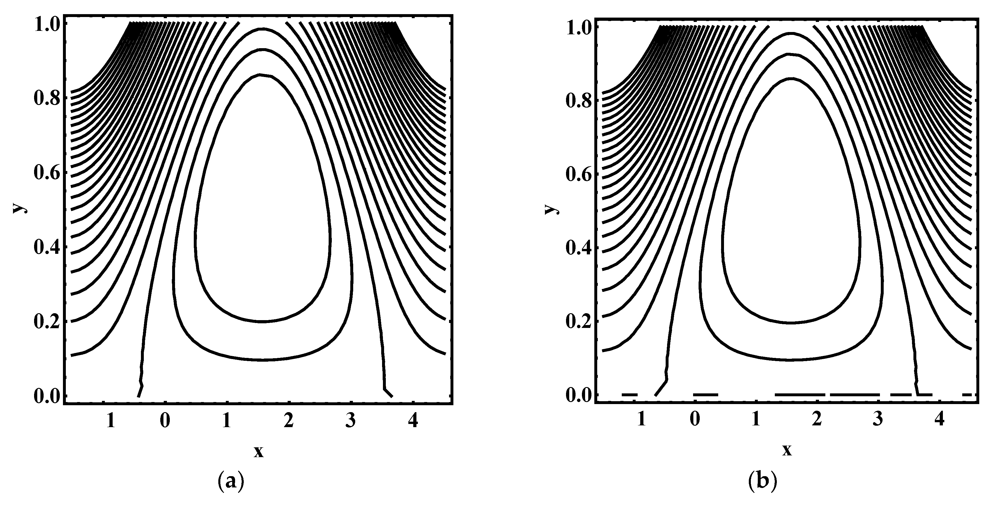
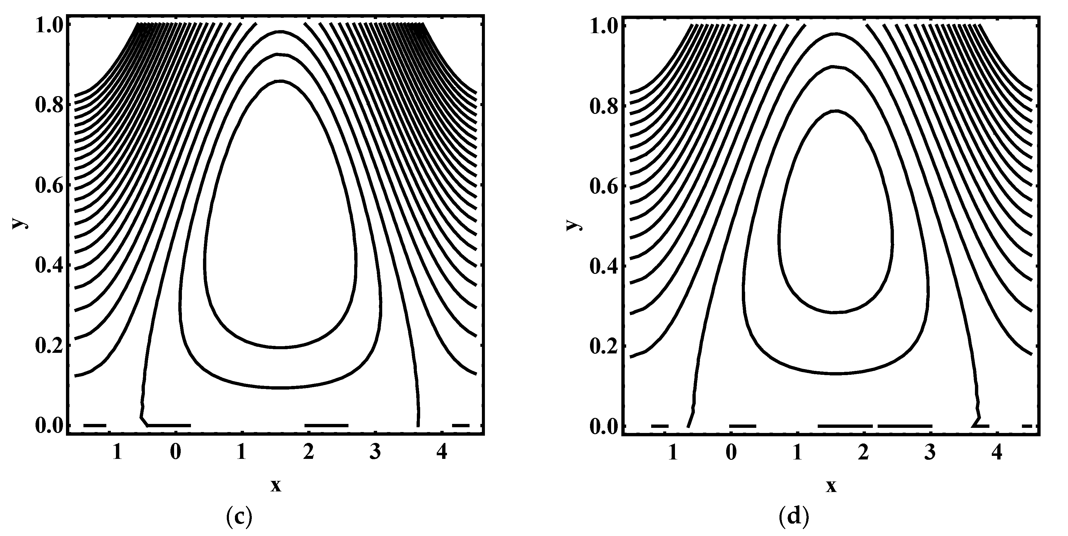
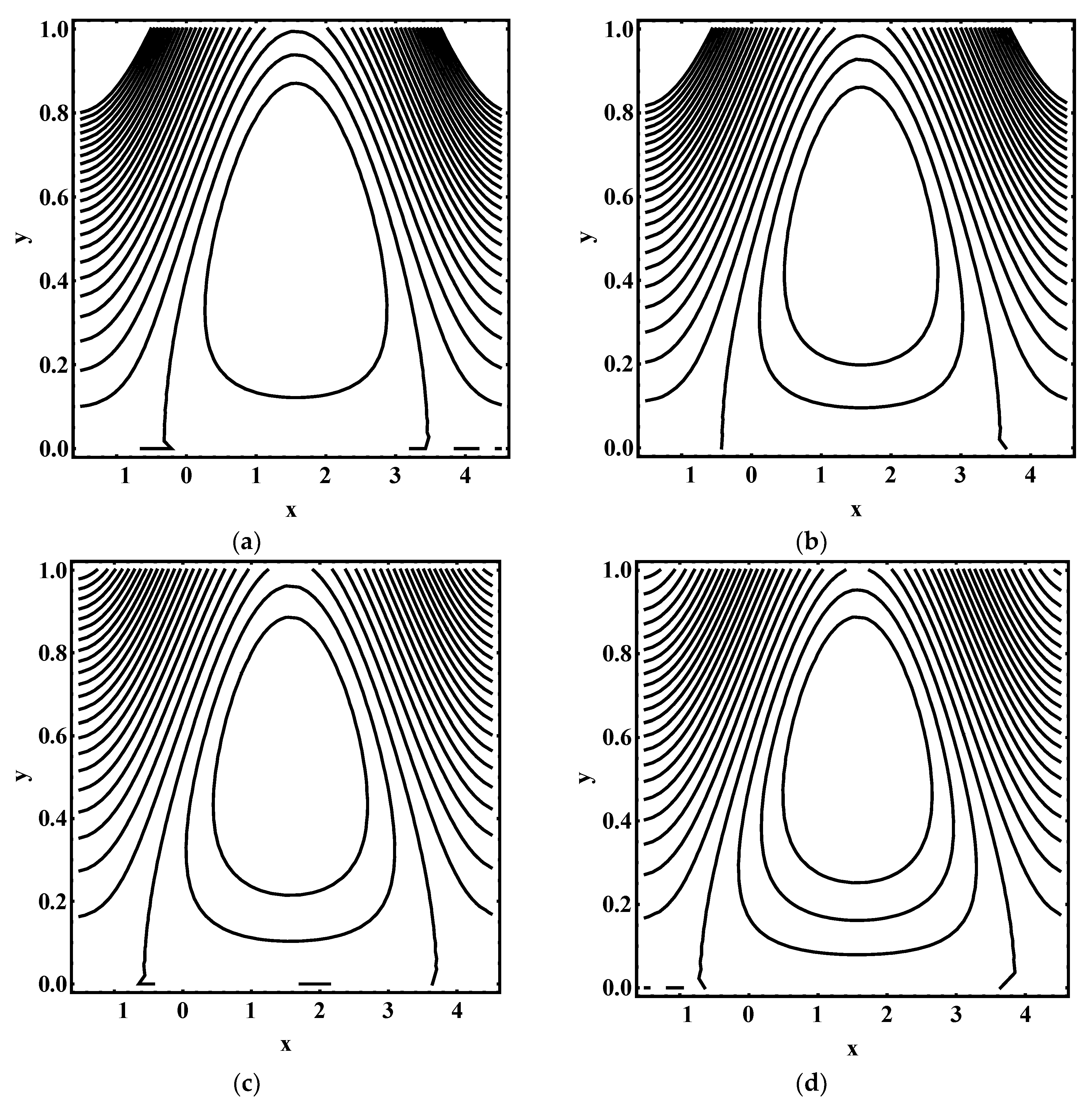
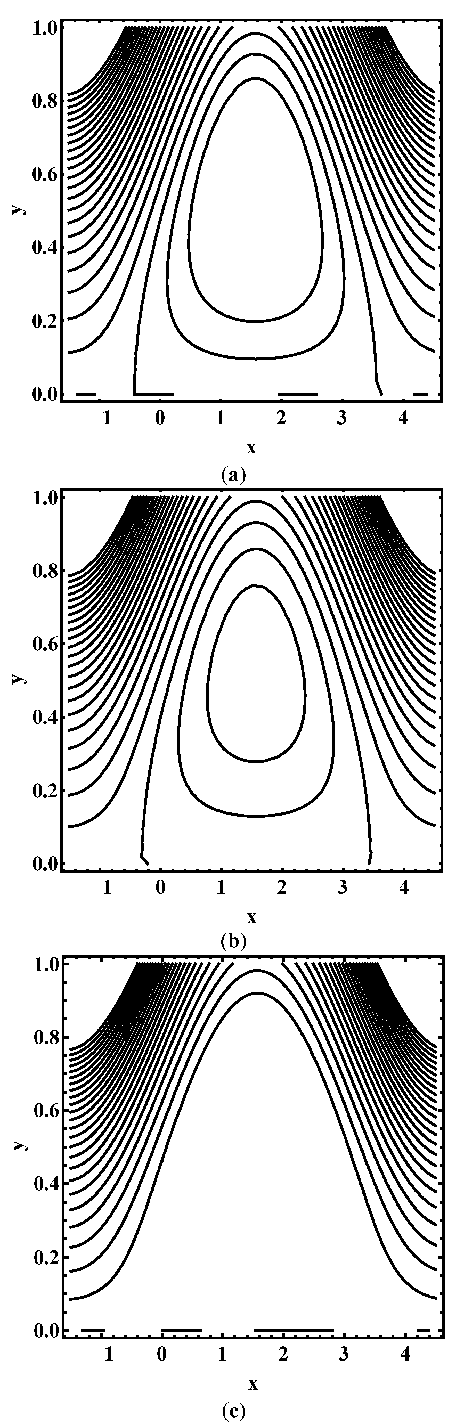
4.4. Trapping Characteristics
Trapping for different values of Deborah number , electroosmotic parameter and maximum electroosmotic velocity are shown in Figure 6, Figure 7 and Figure 8. Figure 6a–d reveal a streamline structure for various values of . The size of the enclosed bolus decreases as increases. It means that size of trapped bolus is strongly affected by changing the fluid. Similarly, Figure 7a–d visualize that the number of enclosed bolus increases with rise in electroosmotic parameter . It scrutinizes that as the increases, the enclosed bolus strongly appears in EDL. It means that more fluid can be trapped in the presence of more electric field. Figure 8a–d illustrate streamline makeup for . It demonstrates that the accumulation of streamline reduces with rise in . Thus, stronger means stronger the external electric field, the number of enclosed significantly decreases for large values of bolus .
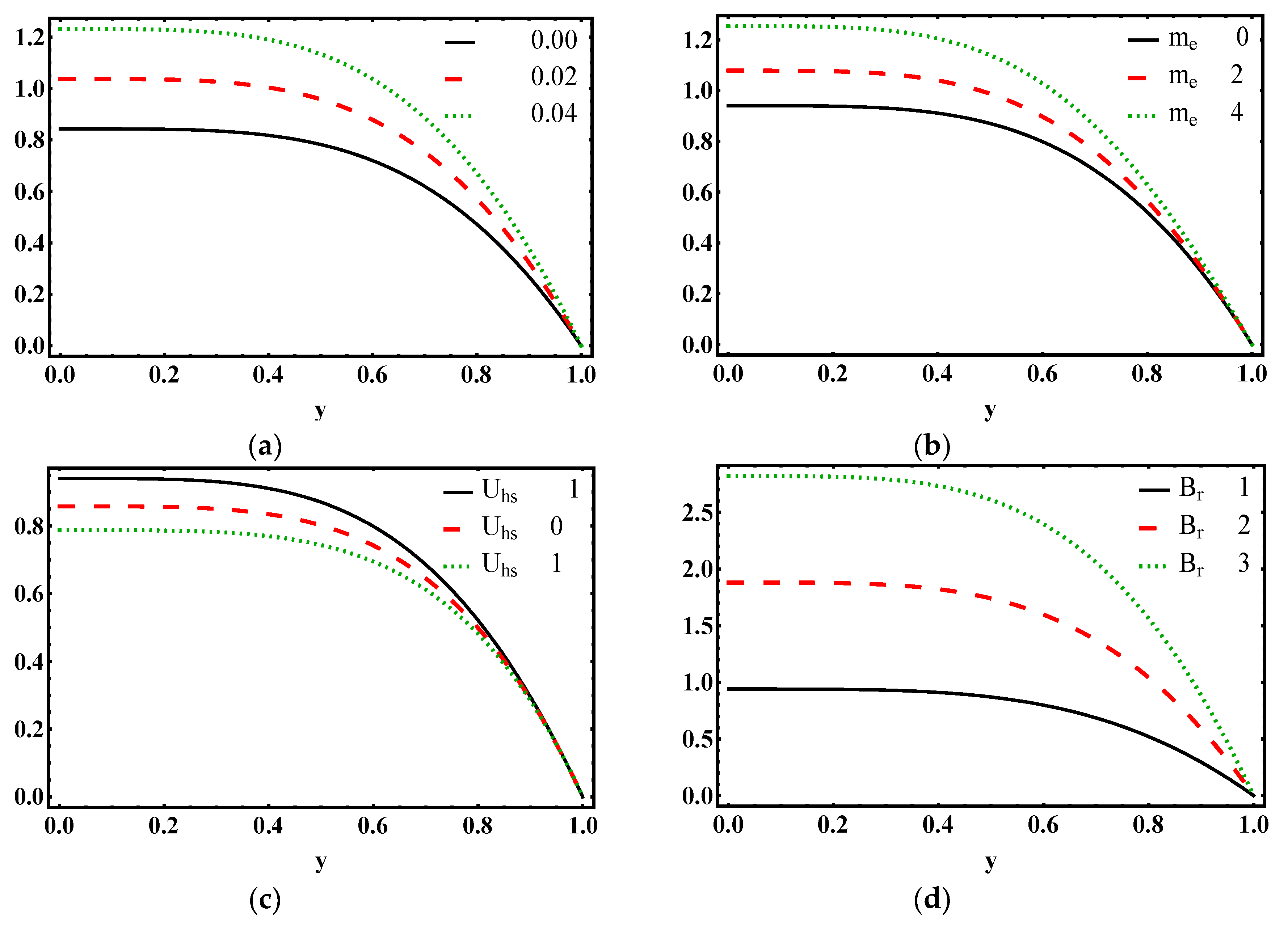
4.5. Temperature Characteristics
In the present subsection, we examined the effect of Deborah number , electroosmotic parameter , maximum electroosmotic velocity and Brinkman number on heat transfer characteristics. Figure 9a reveals the various values of , for temperature distribution It examines that enhances for more values of Also, Figure 9b displays that increases by increasing . Therefore, the decrease in EDL produces a rise in remarkably. Figure 9c, disclose the effects of maximum electroosmotic velocity on . It signifies that for more values of , declines. Figure 9d exemplifies the variation of on i.e., increases for more values of . The main fact in is the viscosity, which creates resistance. This resistance is responsible for the collision of fluid particles and the resulting collision causes an increase in temperature.
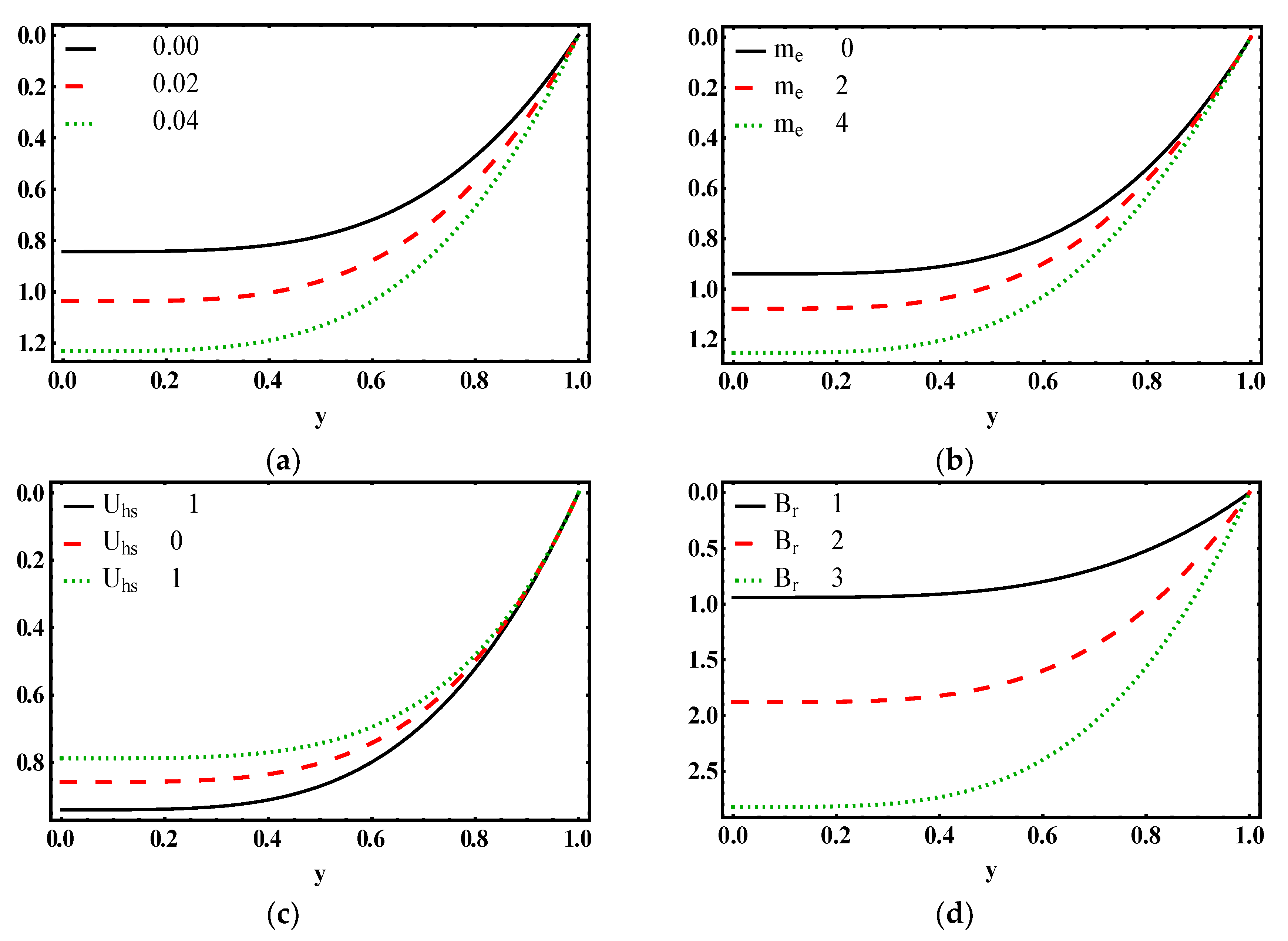
4.6. Concentration Characteristics
Here, we observed the impact of Deborah number , electroosmotic parameter , maximum electroosmotic velocity , Brinkman number , Schmidt number and Soret number on mass transfer characteristics. Figure 10a reveals the various values of , for temperature distribution It examines that decreases for more values of Figure 10b displays that decreases by increasing . Figure 10c discloses the effects of on . It signifies that for more values of , rises. Figure 10d exemplifies the variation of on i.e., decreases for more values of . Figure 10e discloses the effects of on . It implies that decreases for more values of Also, Figure 10f shows that decreases for more values of
4.7. Heat Transfer Coefficient
Figure 11a–d demonstrates the changes in heat transfer coefficient for various values of Deborah number , electroosmotic parameter , maximum electroosmotic velocity , and Brinkman number . This reveals that the various values of , and , the heat transfer coefficient increases. On contrary is decreased for different values of .
4.8. Shear Stress Distribution
Distribution of shear stress provides very useful information about the nature of dissipation at walls. Table 1a–c show the distribution of axial shear stress for different values of Deborah number , maximum electroosmotic velocity and electroosmotic parameter . Table 1a explains that the magnitude of shear stress decreases in the axial direction while it decreases (near the channel wall) then increases (away from channel wall) for different values of Here, it is obvious that the third-grade fluid act as a shear thinning and shear thickening fluid. Similarly, Table 1b displays the variation of shear stress for . It is found that the axial distribution of shear stress enhances for increasing values of . Table 1c presents the shear stress distribution for different values of It is concluded that the same behavior is observed as of . Therefore, we say that the presence of electroosmotic parameter strongly infers the characteristics of third order fluid parameter.
5. Concluding Remarks
From current analysis, we conclude that:
- The axial velocity of third-grade fluid in the microchannel is enhanced due to an increase in electroosmotic parameter.
- For higher values of Schmidt or Soret number, concentration profile decreases.
- The magnitude of pressure rise decreases in the pumping region with the increase of electroosmotic parameter.
- Pressure gradient is more for EOF of third order fluid in comparison to peristaltically flowing fluid.
- Axial distribution of shear stress enhances for increasing values of maximum electroosmotic velocity.
- Volume of trapped bolus is strongly dependent upon the electroosmotic parameter whereas it is suppressed for Deborah number and maximum electroosmotic velocity.
- Temperature distribution in microchannel is crucial for electroosmotic parameter, Deborah number and Brinkman number.
Electro-osmotic exchange of energy and mass has a role in reservoir engineering. The outcomes of the present model may be used by engineers in chemical industry and in micro-fabrication technologies. In the future, this model accompanying porosity will help in understanding the hydrodynamics of rheological fluids in a typical channel employed in a LOC system. This course requires promotion, being of significance in factual life applications.
Author Contributions
Formal analysis, S.N.; Funding acquisition, A.H.; Investigation, S.W.; Methodology, S.W.; Resources, S.N.; Supervision, S.N.; Writing—original draft, S.W.; Writing—review & editing, A.H.
Funding
This research received no external funding. The APC was funded by Ton Duc Thang University, Ho Chi Minh City, Vietnam. However, no grant number is available from source.
Acknowledgments
The third author would like to thank Ton Duc Thang University, Ho Chi Minh City, Vietnam for the financial support.
Conflicts of Interest
The authors declare no conflict of interest.
Nomenclature
| Symbols | Meaning | Dimensions |
| Channel’s half width | [L] | |
| Revilin Erickson tensor | [M/L] | |
| Wave amplitude | [L] | |
| Brinkman number | [-] | |
| Wave speed | [L/T] | |
| Dimensional concentration field | [N/] | |
| , | Concentration field at upper and lower wall | [N/] |
| Diffusivity of chemical species | [-] | |
| Mass diffusivity coefficient | [] | |
| Eckert number | [-] | |
| Axial electric field | [ML/A] | |
| Electron charge | [AT] | |
| Non-dimensional mean flow rate in moving frame | [-] | |
| Dimensional upper wall | [L] | |
| Non-dimensional upper wall | [-] | |
| Thermal conductivity | [ML/K] | |
| Ratio of thermal diffusion | [N/] | |
| Boltzmaan constant | [M/] | |
| Electroosmotic parameter | [-] | |
| Positive and negative ions | [AT] | |
| Bulk concentration | [AT] | |
| Dimensional pressure field | [ML/] | |
| Non-dimensional pressure field | [-] | |
| Peclet number | [-] | |
| Prandtl number | [-] | |
| Dimensional volume flow rate in fixed frame | [/T] | |
| Reynolds number | [-] | |
| Dimensional shear stress | [M/L] | |
| Non-dimensional shear stress | [-] | |
| Schmidt number | [-] | |
| Soret number | [-] | |
| Dimensional time | [T] | |
| Non-dimensional time | [-] | |
| Dimensional temperature field | [K] | |
| , | Temperature field at upper and lower wall | [K] |
| Mean temperature | [K] | |
| Dimensional velocity along direction | [L/T] | |
| Non-dimensional velocity along x direction | [-] | |
| Helmholtz–Smoluchowski velocity | [L/T] | |
| Dimensional velocity along direction | [L/T] | |
| Non-dimensional velocity along y direction | [-] | |
| Dimensional axial coordinate in fixed frame | [L] | |
| Non-dimensional axial coordinate in moving frame | [-] | |
| Dimensional transverse coordinate in fixed frame | [L] | |
| Non-dimensional transverse coordinate in moving frame | [-] | |
| heat transfer coefficient | [-] | |
| Valence of ions | [-] | |
| Peristaltic wave number | [-] | |
| , | Material constants | [-] |
| , | Material constants | [-] |
| Material coefficients | [-] | |
| Wavelength | [L] | |
| Material coefficients | [-] | |
| Debye length | [L] | |
| Dielectric permittivity | [-] | |
| Toatl charge density | [AT/] | |
| Density of fluid | [M/] | |
| Dimensional electric potential | [M] | |
| Non-dimensional electric potential | [-] | |
| Non-dimensional Deborah number | [-] | |
| Amplitude ratio | [-] | |
| Non-dimensional volume flow rate | [-] | |
| Non-dimensional temperature field | [-] | |
| Non-dimensional concentration field | [-] | |
| Dimensional stream function | [/T] | |
| Non-dmensional stream function | [-] |
Appendix A
References
- Huang, X.; Gordon, M.J.; Zare, R.N. Current-monitoring method for measuring the electroosmotic flow rate in capillary zone electrophoresis. Anal. Chem. 1998, 60, 1837–1838. [Google Scholar] [CrossRef]
- Gravesen, P.; Branebjerg, J.; Jensen, O.S. Microfluidics-a review. J. Micromech. Microeng. 1993, 3, 168. [Google Scholar] [CrossRef]
- Haswell, S.J. Development and operating characteristics of micro flow injection based on electroosmotic flow. Analyst 1997, 122, 1R–10R. [Google Scholar] [CrossRef]
- Patankar, N.A.; Hu, H.H. Numerical simulation of electroosmotic flow. Anal. Chem. 1998, 70, 1870–1881. [Google Scholar] [CrossRef] [PubMed]
- Kang, Y.; Yang, C.; Huang, X. Electroosmotic flow in a capillary annulus with high zeta potentials. J. Colloid Interface Sci. 2002, 253, 285–294. [Google Scholar] [CrossRef] [PubMed]
- Hayat, T.; Abbasi, F.M. Variable viscosity effects on the peristaltic motion of a third-order fluid. Int. J. Numer. Methods Fluids 2011, 67, 1500–1515. [Google Scholar] [CrossRef]
- Noreen, S. Mixed convection peristaltic flow of third order nanofluid with an induced magnetic field. PLoS ONE 2013, 8, e78770. [Google Scholar] [CrossRef]
- Noreen, S. Effects of joule heating and convective boundary conditions on magnetohydrodynamic peristaltic flow of couple-stress fluid. J. Heat Transf. 2016, 138, 094502. [Google Scholar] [CrossRef]
- Prakash, J.; Siva, E.P.; Balaji, N.; Kothandapani, M. Effect of peristaltic flow of a third-grade fluid in a tapered asymmetric channel. J. Phys. 2018, 1000, 012165. [Google Scholar] [CrossRef]
- Mallick, B.; Misra, J.C. Peristaltic flow of Eyring-Powell nanofluid under the action of an electromagnetic field. Eng. Sci. Technol. 2019, 22, 266–281. [Google Scholar] [CrossRef]
- Chakraborty, S. Augmentation of peristaltic microflows through electro-osmotic mechanisms. J. Phys. D Appl. Phys. 2006, 39, 5356. [Google Scholar] [CrossRef]
- Tang, G.H.; Li, X.F.; He, Y.L.; Tao, W.Q. Electroosmotic flow of non-Newtonian fluid in microchannels. J. Non-Newton. Fluid Mech. 2009, 157, 133–137. [Google Scholar] [CrossRef]
- Hadigol, M.; Nosrati, R.; Nourbakhsh, A.; Raisee, M. Numerical study of electroosmotic micromixing of non-Newtonian fluids. J. Non-Newton. Fluid Mech. 2011, 166, 965–971. [Google Scholar] [CrossRef]
- Yavari, H.; Sadeghi, A.; Saidi, M.H.; Chakraborty, S. Temperature rise in electroosmotic flow of typical non-Newtonian biofluids through rectangular microchannels. J. Heat Transf. 2014, 136, 031702. [Google Scholar] [CrossRef]
- Bandopadhyay, A.; Tripathi, D.; Chakraborty, S. Electroosmosis-modulated peristaltic transport in microfluidic channels. Phys. Fluids 2016, 28, 052002. [Google Scholar] [CrossRef]
- Jiang, Y.; Qi, H.; Xu, H.; Jiang, X. Transient electroosmotic slip flow of fractional Oldroyd-B fluids. Microfluid. Nanofluid. 2017, 21, 7. [Google Scholar] [CrossRef]
- Jhorar, R.; Tripathi, D.; Bhatti, M.M.; Ellahi, R. Electroosmosis modulated biomechanical transport through asymmetric microfluidics channel. Indian J. Phys. 2018, 92, 1229–1238. [Google Scholar] [CrossRef]
- Tripathi, D.; Yadav, A.; Bég, O.A.; Kumar, R. Study of microvascular non-Newtonian blood flow modulated by electroosmosis. Microvasc. Res. 2018, 117, 28–36. [Google Scholar] [CrossRef]
- Francesko, A.; Cardoso, V.F.; Lanceros-Méndez, S. Lab-on-a-chip technology and microfluidics. In Microfluidics for Pharmaceutical Applications; William Andrew: Norwich, UK, 2019; pp. 3–36. [Google Scholar]
- Jayavel, P.; Jhorar, R.; Tripathi, D.; Azese, M.N. Electroosmotic flow of pseudoplastic nanoliquids via peristaltic pumping. J. Braz. Soc. Mech. Sci. 2019, 41, 61. [Google Scholar] [CrossRef]
- Sadeghi, A.; Saidi, M.H.; Mozafari, A.A. Heat transfer due to electroosmotic flow of viscoelastic fluids in a slit microchannel. Int. J. Heat Mass Transf. 2011, 54, 4069–4077. [Google Scholar] [CrossRef]
- Babaie, A.; Saidi, M.H.; Sadeghi, A. Heat transfer characteristics of mixed electroosmotic and pressure driven flow of power-law fluids in a slit microchannel. Int. J. Therm. Sci. 2012, 53, 71–79. [Google Scholar] [CrossRef]
- Chen, C.H.; Hwang, Y.L.; Hwang, S.J. Non-Newtonian fluid flow and heat transfer in microchannels. Appl. Mech. Mater. 2013, 275, 462–465. [Google Scholar] [CrossRef]
- Sinha, A.; Shit, G.C. Electromagnetohydrodynamic flow of blood and heat transfer in a capillary with thermal radiation. J. Magn. Magn. Mater. 2015, 378, 143–151. [Google Scholar] [CrossRef]
- Shit, G.C.; Mondal, A.; Sinha, A.; Kundu, P.K. Electro-osmotically driven MHD flow and heat transfer in micro-channel. Physica A 2016, 449, 437–454. [Google Scholar] [CrossRef]
- Bhatti, M.M.; Zeeshan, A.; Ellahi, R.; Ijaz, N. Heat and mass transfer of two-phase flow with Electric double layer effects induced due to peristaltic propulsion in the presence of transverse magnetic field. J. Mol. Liq. 2017, 230, 237–246. [Google Scholar] [CrossRef]
- Reddy, K.V.; Makinde, O.D.; Reddy, M.G. Thermal analysis of MHD electro-osmotic peristaltic pumping of Casson fluid through a rotating asymmetric micro-channel. Indian J. Phys. 2018, 92, 1439–1448. [Google Scholar] [CrossRef]
- Yadav, A.; Bhushan, S.; Tripathi, D. Peristaltic pumping through porous medium in presence of electric double layer. EDP Sci. 2018, 192, 02043. [Google Scholar] [CrossRef]
- Narla, V.K.; Tripathi, D.; Sekhar, G.R. Time-dependent analysis of electroosmotic fluid flow in a microchannel. J. Eng. Math. 2019, 114, 177–196. [Google Scholar] [CrossRef]
- Yang, C.; Jian, Y.; Xie, Z.; Li, F. Heat transfer characteristics of magnetohydrodynamic electroosmotic flow in a rectangular microchannel. Eur. J. Mech. B-Fluids 2019, 74, 180–190. [Google Scholar] [CrossRef]
Figure 1.
Schematic of the geometry of electro-osmotically modulated peristaltic flow.

Figure 2.
Comparative analysis between Perturbation solution and Numerical solution for axial velocity, while other parameters are .
Figure 2.
Comparative analysis between Perturbation solution and Numerical solution for axial velocity, while other parameters are .

Figure 3.
Axial velocity u profile for . , while other parameters are .

Figure 4.
Pressure rise profile for . , while other parameters are .

Figure 5.
Pressure gradient profile for , while other parameters are .

Figure 6.
Streamline distribution for . , while other parameters are .


Figure 7.
Streamline distribution for . , while other parameters are .

Figure 8.
Streamline distribution for . , while other parameters are .

Figure 9.
Temperature profile for , while other parameters are .

Figure 10.
Concentration profile for . while other parameters are .

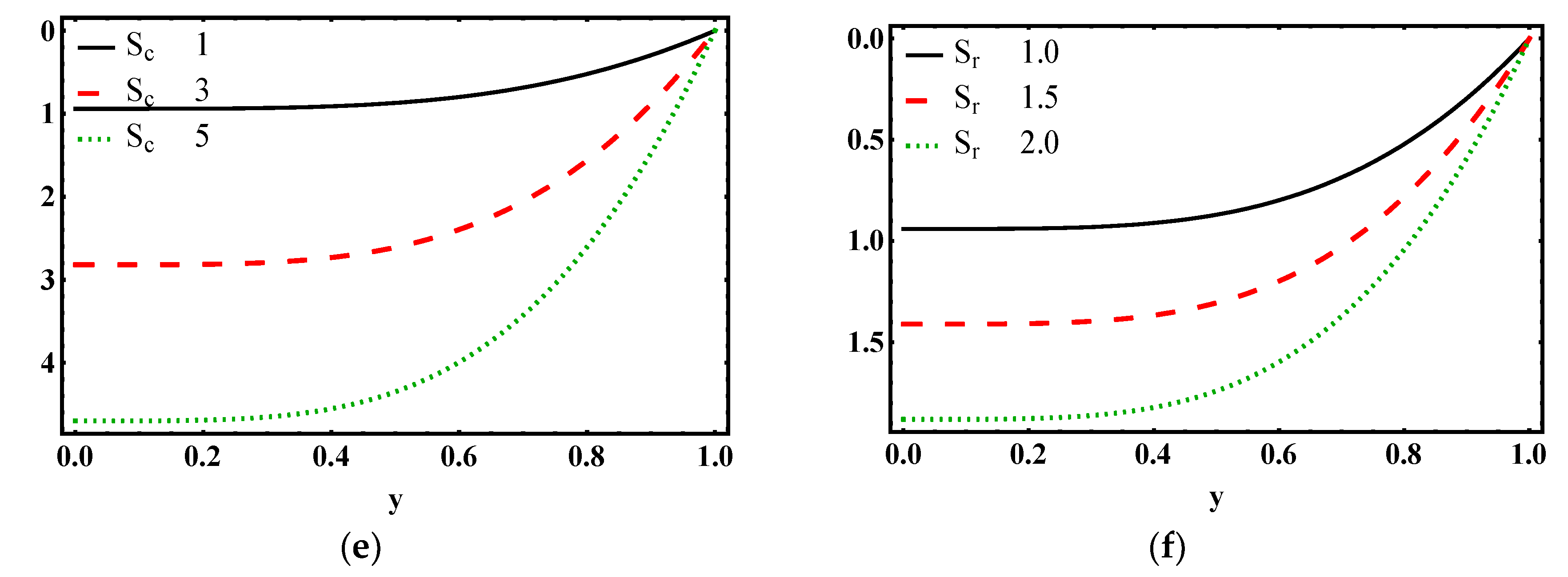
Figure 11.
Heat transfer coefficient for , while other parameters are .


Table 1.
Numerical values of shear stress at the wall for different values of Deborah number , Helmholtz–Smoluchowski velocity and electroosmotic parameter .
Table 1.
Numerical values of shear stress at the wall for different values of Deborah number , Helmholtz–Smoluchowski velocity and electroosmotic parameter .
| (a) | |||
| 0.0 | 0.2 | 0.4 | |
| 0.1 | −2.4917 | −3.0742 | −0.8223 |
| 0.2 | −2.3669 | −3.8790 | −2.2711 |
| 0.3 | −2.6497 | −4.5689 | −4.3309 |
| (b) | |||
| −1.0 | 0.0 | 1.0 | |
| 0.1 | −3.6869 | −1.1370 | 0.5727 |
| 0.2 | −3.7974 | −1.2903 | 0.4311 |
| 0.3 | −3.8395 | −1.4188 | 0.3188 |
| (c) | |||
| 2 | 4 | 6 | |
| 0.1 | −3.6869 | −10.778 | −6.3530 |
| 0.2 | −3.7974 | −8.7149 | −4.7301 |
| 0.3 | −3.8395 | −7.0505 | −3.6590 |
© 2019 by the authors. Licensee MDPI, Basel, Switzerland. This article is an open access article distributed under the terms and conditions of the Creative Commons Attribution (CC BY) license (http://creativecommons.org/licenses/by/4.0/).
Share and Cite
MDPI and ACS Style
Waheed, S.; Noreen, S.; Hussanan, A. Study of Heat and Mass Transfer in Electroosmotic Flow of Third Order Fluid through Peristaltic Microchannels. Appl. Sci. 2019, 9, 2164. https://doi.org/10.3390/app9102164
AMA Style
Waheed S, Noreen S, Hussanan A. Study of Heat and Mass Transfer in Electroosmotic Flow of Third Order Fluid through Peristaltic Microchannels. Applied Sciences. 2019; 9(10):2164. https://doi.org/10.3390/app9102164
Chicago/Turabian StyleWaheed, Sadia, Saima Noreen, and Abid Hussanan. 2019. "Study of Heat and Mass Transfer in Electroosmotic Flow of Third Order Fluid through Peristaltic Microchannels" Applied Sciences 9, no. 10: 2164. https://doi.org/10.3390/app9102164
Note that from the first issue of 2016, this journal uses article numbers instead of page numbers. See further details here.