Abstract
Barrett’s esopaghagus (BE) is a known precursor of esophageal adenocarcinoma (EAC). Patients with BE undergo regular surveillance to early detect stages of EAC. Volumetric laser endomicroscopy (VLE) is a novel technology incorporating a second-generation form of optical coherence tomography and is capable of imaging the inner tissue layers of the esophagus over a 6 cm length scan. However, interpretation of full VLE scans is still a challenge for human observers. In this work, we train an ensemble of deep convolutional neural networks to detect neoplasia in 45 BE patients, using a dataset of images acquired with VLE in a multi-center study. We achieve an area under the receiver operating characteristic curve (AUC) of 0.96 on the unseen test dataset and we compare our results with previous work done with VLE analysis, where only AUC of 0.90 was achieved via cross-validation on 18 BE patients. Our method for detecting neoplasia in BE patients facilitates future advances on patient treatment and provides clinicians with new assisting solutions to process and better understand VLE data.
1. Introduction
Esophageal adenocarcinoma (EAC) is among the most common and lethal cancers in the world. EAC has shown a rapid increase since the late 1980s and it is estimated that the number of new esophageal cancer cases will be doubled by 2030 [1]. Barrett’s esophagus (BE) is a condition in which normal squamous epithelium at the distal end of the esophagus is replaced by metaplastic columnar epithelium due to overexposure to gastric acid and it is associated with an increased risk of developing EAC [2]. For this reason, patients diagnosed with BE currently undergo regular surveillance with white-light endoscopy (WLE) with the aim to detect early high-grade dysplasia (HGD) and intramucosal adenocarcinoma. It is important to detect these lesions early, as curative treatment is still possible at this stage by a minor endoscopic intervention. However, early neoplastic lesions are regularly missed because of their subtle appearances, or as a result of sampling errors during biopsy [3,4,5].
Volumetric laser endomicroscopy (VLE) is a novel advanced imaging system with the potential to early detect suspicious areas containing BE, which may be regularly missed with current white-light endoscopy. VLE incorporates a second-generation form of optical coherence tomography (OCT) technology. Improvements in image acquisition speed enable this balloon-based system to perform a quick circumferential scan of the entire distal esophagus. VLE provides a three-dimensional map of near-microscopic resolution of the subsurface layers of the esophagus over a length of 6 cm and depth of 3 mm into the tissue. However, a VLE scan generates a large amount of gray-shaded data (i.e., typically 1200 cross-sectional images or frames of pixels) that need to be analyzed in real time during endoscopy.
In recent studies [6,7], clinical VLE prediction models were developed for BE neoplasia with successful accuracy results. Several visual VLE features (lack of layering, high surface signal intensity, and irregular glandular architecture) were identified as possible indicators of BE neoplasia by comparing VLE-histology correlated images from 25 ex-vivo specimens. However, follow-up studies using ex-vivo [8] and in-vivo [9] VLE data suggested that full-scan VLE interpretation by experts remains a challenge. Computer aided diagnosis (CADx) systems offer relevant assistance in clinical decision making. In van der Sommen et al. [10], a CADx system was developed for the detection of early BE neoplasia on WLE images. Early work in endoscopic optical coherence tomography (EOCT) was shown in Qi et al. [11,12], where a CADx system based on multiple feature extraction methods was developed to detect neoplasia in BE patients in a dataset of EOCT biopsies. Similar related work was performed by Ughi et al. [13], where a system was developed to automatically characterize and segment the esophageal wall of patients with BE using tethered capsule endomicroscopy (TCE).
The first related work performed on VLE was presented in Swager et al. [14], where a CADx system was developed to detect early BE neoplasia on 60 VLE images from a database of high-quality ex-vivo VLE-histology correlations (30 non-dysplastic BE (NDBE) and 30 neoplastic images, containing HGD or early EAC). In their work, two novel clinically-inspired quantitative image features specific for VLE were developed based on the VLE surface signal and the intensity histogram of several layers. Recently, additional work was performed by Scheeve et al. [15], where another novel clinically-inspired quantitative image feature was developed based on the glandular architecture, and analyzed in a dataset of 18 BE patients with and without early BE neoplasia (88 NDBE and 34 HGD/EAC). Both studies investigated the features using several machine learning methods, such as support vector machine, random forest or AdaBoost, and showed successful results towards BE neoplasia assessment. However, the results were only obtained in a small patient population (29 endoscopic resections and 18 VLE laser-marked regions of interest (ROIs), respectively), suggesting that a larger dataset might be needed to further validate and possibly improve the results.
In this study, we extend the work of Scheeve et al. [15] by using a larger dataset of 45 patients, and we incorporate current state-of-the-art deep learning techniques to improve the classification of non-dysplastic and neoplastic BE patients. To the best of our knowledge, this is the first study applying deep convolutional neural networks (DCNNs) for early BE neoplasia classification on patients acquired with in-vivo VLE. The results are compared with previously developed clinically-inspired features specific for VLE, and validated on a test dataset that is unseen during training time.
2. Materials and Methods
2.1. VLE Imaging System
The Nvision VLE Imaging System (NinePoint Medical, Inc., Bedford, MA, USA) integrates a second-generation form of OCT technology, termed optical frequency-domain imaging (OFDI) [16,17,18,19]. The VLE system was composed of a disposable optical probe with an inflation system and an imaging console, which incorporates a swept light source, optical receiver, interferometer, and a data-acquisition computer. The light source consisted of a near infrared light ( = 1250–1350 nm) that was transmitted into the catheter. At the distal end of the optical probe, a non-compliant balloon allowed a correct alignment in the esophagus for in-vivo imaging. During an automatic pullback of the optical probe, a 6 cm circumferential segment of the esophagus is scanned in 90 seconds. A VLE pullback acquires 1200 cross-sectional images with a sampling density of 50 μm (voxel dimensions, ). The axial and lateral resolution of a VLE image were approximately 7 and 40 , respectively. The penetration depth reached approximately 3 into tissue. For more comprehensive technical details we refer to previous publications [16,17,18,19].
2.2. Data Collection and Description
In a prospective multi-center clinical study, for the PREDICTion of BE neoplasia (PREDICT study), VLE data was acquired in vivo from 45 patients undergoing BE surveillance at the Amsterdam UMC (AMC; Amsterdam, The Netherlands), the Catharina Hospital (CZE; Eindhoven, The Netherlands), and the St. Antonius Hospital (ANZ; Nieuwegein, The Netherlands) from October 2017 to November 2018, using a commercial VLE system (NinePoint Medical, Inc., Bedford, MA, USA). Patients undergoing surveillance of NDBE, or patients referred for work-up and treatment of BE with early neoplasia (HGD and/or EAC), were eligible for this study. The study was approved by the institutional review boards at AMC, CZE, and ANZ. Written informed consent was obtained from all patients prior to VLE imaging.
For each patient, one or several regions of interest (ROIs) were extracted in the following manner. First, four-quadrant laser-mark pairs were placed at 2 cm intervals using the VLE system, according to the Seattle biopsy protocol [20,21]. Next, a full VLE scan was performed, after which the VLE balloon was retracted from the esophagus. Then, regular endoscopy was used to obtain biopsies in between the laser-mark pairs. Finally, ROIs were cropped from the full scan in between the same laser-mark pairs, and were labeled according to pathology outcome, ensuring histology-correlation [22] of the extracted ROIs. The histopathological correlation was assumed to apply over , conform a small biopsy specimen, comprising 25 cross-sectional images, in both vertical directions (i.e., distal and proximal), and thus resulting in 51 images per ROI.
In total, 233 NDBE and 80 neoplastic (HGD/EAC) ROIs were laser-marked under VLE guidance and subsequently biopsied for histological evaluation by an expert pathologist for BE. Out of the total cohort of patients, the first 22 patients were used as the training dataset (134 NDBE and 38 HGD/EAC ROIs, totalling 8772 VLE images) and the remaining 23 were treated as the unseen test dataset (99 NDBE and 42 HGD/EAC ROIs, totalling 7,191 VLE images).
2.3. Clinically-Inspired Features for Multi-Frame Analysis
In the previous works of Klomp et al. [23] and Scheeve et al. [15], several clinically-inspired quantitative image features were developed, the layer histogram (LH) and gland statistics (GS), to detect BE neoplasia in single frames. We referred to analysing one VLE image in a ROI to predict BE neoplasia as single-frame analysis. In Scheeve et al. [15], a single VLE image per ROI was used to compute the resulting prediction for each ROI. For a fair comparison with these studies, and per our request to the authors, we present our results by extending the single-frame analysis to 51 VLE images per ROI, further referred to as multi-frame analysis. The development of the clinically-inspired features has been described previously [15,23,24]. A summary of the methodology for the multi-frame analysis is given in the following sections.
2.3.1. Preprocessing
Relevant tissue regions were segmented from VLE images, removing regions not suitable for analysis, such as regions of air and deeper tissue with a low signal-to-noise ratio. The tissue segmentation masks were obtained using FusionNet with a domain-specific loss function [25]. Using these segmentation masks, tissues of interest (TOIs) were segmented and flattened, by extracting the first 200 pixels (i.e., approximately 1 of tissue) from the top of each column that is indicated by the tissue segmentation mask [24].
2.3.2. Layer Histogram and Gland Statistics
From the flattened TOI data, the LH feature was computed. The LH feature captures the (lack of) layering in the VLE data by computing the N-bin histograms of the first M layers of d pixels, starting from the top of the flattened TOI data [23,24]. To detect glandular structures in the flattened TOI data, gland segmentation masks were computed using a simple segmentation algorithm, involving local adaptive thresholding and basic morphological operations. After glands were detected, the GS feature was computed, which captures the characteristics of glandular structures in the VLE data. This GS feature comprises features for (1) texture analysis, (2) geometry analysis, as well as (3) VLE-specific information [15]. Both LH and GS capture characteristics in the VLE data that are indicative for dysplasia [7,26].
2.4. Ensemble of Deep Convolutional Neural Networks
In recent years, deep convolutional neural networks (DCNNs) have shown to be highly effective for segmentation, classification, and learning specific patterns in images. In the paradigm of optical coherence tomography (OCT), DCNNs have been successfully applied to OCT, such as segmentation of retinal layers [27] and macular edema [28], detection of macular fluid [29], or treatment of age-related macular degeneration [30,31]. In this section we present our approach with DCNNs in a dataset of in-vivo VLE images for the classification of neoplasia in patients with BE.
2.4.1. Preprocessing VLE
In order to guide the network towards a better convergence, and similar to single-frame analysis (Section 2.3.1), we performed some specific cleaning by removing non-informative areas from the original VLE images. This removal involved two main sources of less important information: (1) the pixel background information, and (2) the balloon pixel information. Our aim was to maximize the useful information that the network can learn and exclude any additional learning that degrades the classification task. For this reason each image was cropped to occlude the balloon. For each VLE image, the balloon region (Figure 1, red curve) was removed following the steps below:
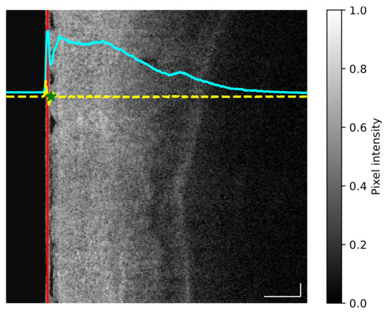
Figure 1.
(Best viewed in color) Example of preprocessing applied to each volumetric laser endomicroscopy (VLE) frame. At the left side of the image the balloon line (red line) is located by calculating the average intensity of the whole image (cyan line) and then using the first derivative (yellow line) to extract the end point of the balloon pixel (green star). Scale bars: 0.5 mm.
- For each image the average intensity curve was computed along the vertical dimension, thus allowing us to obtain the profile of changing intensity (Figure 1, cyan curve).
- The first derivative of the average intensity curve was computed to obtain a quantitative measurement of slope differences (Figure 1, yellow curve).
- Given the first derivative, the balloon end location was defined as the local maximum value found after the minimum point of the first derivative (Figure 1, green star).
2.4.2. Preprocessing DCNN
Each of the networks were initialized using pre-trained ImageNet weights [32]. One limitation of using a pre-trained model is that the associated architecture cannot be changed, since the weights are originally trained for a specific input configuration. Hence to match the requirements of the pre-trained ImageNet weights, each image was resized to pixels. In addition, the dataset was normalized by subtracting the mean and dividing by the standard deviation specified by the pre-trained ImageNet weights. As a final step, the gray-scale channel of each VLE image was triplicated to simulate the RGB input requirement of the pre-trained model (Figure 2).
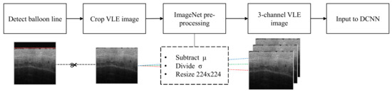
Figure 2.
Automatic workflow of the preprocessing applied to each VLE frame. First the balloon line is detected in the VLE frame. Secondly, the image is cropped below the detected balloon line. The VLE image is then resized to . The mean () is subtracted and the standard deviation ( ) divided according to the pre-trained ImageNet weights. Finally, the gray-scale channel is then triplicated to simulate the RGB requirements of the pre-trained network.
2.4.3. Data Split of the Training Dataset
For separating training and validation datasets, we propose to split the data according to the patient neoplasia-basis, rather than splitting data on frame-basis. Splitting on frame-basis cannot be done naively, since the frames are highly correlated in the following way. Each (multi-frame) ROI of the training dataset (22 patients of the PREDICT study) contains a total of 51 frames comprising roughly 2.5 mm of the total 6 cm length of the scanned esophagus. Succeeding frames are therefore highly correlated and contain nearly the same data. The only remaining option therefore is splitting data on patient neoplasia-basis. To avoid overfitting, the patient distribution for each neoplasia grade was analyzed.
In Table 1, we show the number of patients that belong to each class, as well as the number of ROIs pathologically confirmed as non-dysplastic and dysplastic. We can observe that three patients share the NDBE and HGD class label, therefore we decided to split our datasets in three groups. To avoid patient bias during training, we select only ROIs from NDBE and HGD and data from one patient that have both. This leads to three permuted datasets. Given this permutation, we have trained three individual DCNNs, which together is called an ensemble of networks. When evaluated in the external test dataset, the resulting ensemble of the three networks is used to obtain the probability of an ROI belonging to NDBE or HGD, further explained in Section 3.

Table 1.
Class distribution based on the regions of interest (ROIs) of the training dataset of the first 22 patients.
2.4.4. DCNN Description
In this section we present the choice of the network architecture and motivate why it best fits our data. In this work we utilized an ensemble of networks, each of them based on the VGG16 architecture proposed by Simoyan et al. [33]. We have found that due to the unbalanced nature of the data, a simple but yet deep model was the most effective way to classify our VLE images. Deep models are useful to learn complex features, but at the cost of a large amount of parameters to train and slow inference time.
Figure 3 depicts the architecture of the DCNN, based on the VGG16 network. VGG16 is composed of five groups of convolutional blocks with a maxpooling layer at the end of each block. In the original architecture, the classification layer was wrapped into two fully connected (FC) layers followed by the classification layer with a softmax activation. In our work, we added a global average pooling (GAP) layer (Figure 3, blue block) after the last convolutional block, which reduced the amount of learnable parameters from to . The GAP layer was followed by a fully connected layer of 512 hidden units instead of 4096 proposed in the original VGG16 network. Subsequently, a dropout layer () was added to the architecture, followed by the final classification layer with a softmax activation.
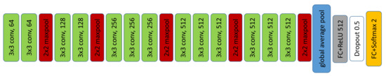
Figure 3.
Architecture of the deep convolutional neural network (DCNN) used in this study, which is based on VGG16.
2.4.5. Training
We have fine-tuned the VGG16 of each ensemble-network by freezing the first four convolutional blocks. Stochastic gradient descent (SGD) was chosen as optimizer with momentum (). We opted for using an adaptive learning rate via cosine annealing with restarts. The learning rate fluctuated between 1e-3 and 1e-6. The learning cycle was repeated every two epochs. Furthermore, to alleviate imbalanced data between both classes, we have enforced an equal distribution of classes for each epoch. We have chosen a batch size of 100, equally sampling both classes. For each image, several data augmentations were applied, to enrich the generalization of the network and to avoid overfitting. We chose to use a combination of horizontal flip, motion blur and optical grid distortion, which in our opinion best represents the behaviour of VLE images with in-vivo data exploration. The three DCNNs were trained until convergence was achieved.
3. Results
The results in this section are divided in three parts: (A) clinical feature comparison of single-frame analysis and multi-frame performance, (B) performance of the three DCNNs and its ensemble, and (C) comparison of our work with the literature.
A. Clinical feature comparison. In this section we report the results obtained in the multi-frame analysis provided per our demand to the authors of Scheeve et al. [15]. We compared the multi-frame classification results with the single-frame work. The multi-frame analysis for the LH feature achieved an average area under the receiver operating characteristic curve (AUC) of compared to the single-frame analysis, which achieved an AUC of . In the same manner, the GS feature achieved an average AUC of for the multi-frame analysis, in comparison with an average AUC of for the single-frame methodology. Overall, we observe that the GS feature does not achieve better performance than the single-frame technique. Alternatively, we saw an increased performance on the LH feature when the multi-frame analysis is applied (AUC 0.90 vs. 0.86).
B. Performance of the three DCNNs and its ensemble. In order to validate the ensemble of DCNNs, we have evaluated our approach using the unseen test dataset. The posterior probabilities were computed for each VLE frame using the three trained DCNNs. For each ROI, a total of 51 possible predictions were obtained for each DCNN. The final probability of an ROI belonging to NDBE or HGD was computed by averaging the total number of probabilities in each DCNN, reported as the multi-frame probability. In Equation (1), the multi-frame probability can be explained as the decision of an ROI belonging to certain class A, computed by averaging the total probabilities of M frames for a number of N networks, where in our case and .
Given a multi-frame probability, we computed accuracy metrics for both the training dataset and the test dataset. Additionally we computed the sensitivity, defined as the rate of HGD ROIs that are correctly identified as such (true positives), and specificity, defined as the proportion of NDBE ROIs that are correctly identified as such (true negatives). The receiver operating characteristic curve (ROC) was computed as well for both datasets for each trained DCNN. In Table 2, we present the results of the ensemble of DCNNs. To showcase the efficacy of our method, we report the classification results using the single-frame and multi-frame analysis for each of the training dataset and the test dataset. All metrics are reported with confidence intervals (CIs) at 95%. All presented values are reported at the optimal threshold setting, which was calculated from the training dataset.
Table 2.
Comparison of single-frame and multi-frame analysis using the ensemble deep convolutional neural network (DCNN) for both the training and the test dataset.
We observe that similar to the results presented in Section 3, we obtain an increased performance when accounting the multi-frame probability for both the training dataset (AUC, 0.98 vs. 0.95) and the test dataset (AUC, 0.96 vs. 0.90). Figure 4 portrays the computed ROC for the test dataset and the associated confusion matrix. The ROC curve was computed for each trained DCNN and the total ensemble. It shows that the combination of the three DCNNs improves the performance of our model (AUC, 0.96 vs. 0.92–0.96) (Figure 4a).
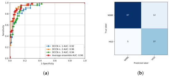
Figure 4.
(a) Receiver operating characteristic curve for the three trained networks and the resulting ensemble validated on the external dataset. AUC denotes the area under the receiver operating characteristic curve. (b) Resulting confusion matrix for the external dataset.
C. Comparison of our work with the literature. Previous work done in VLE images [14,15] focused on extracting features to detect neoplasia in BE patients. To compare with the literature, we have extended the work of Scheeve et al. [15] for multi-frame analysis. In Table 3, we compare our results with recent work on VLE, as well as highlight the nature of each of the studies. Our study is based on experiments with a more robust dataset, provided by increasing to 45 the number of BE patients, which allows the DCNN to learn a wider range of features. Moreover, we show that using a multi-frame approach for classifying an ROI increases the confidence of our algorithm, compared to single-frame analysis (0.90 vs 0.86 with Scheeve et al. [15] method, and 0.96 vs 0.91 with our proposed DCNN).
Table 3.
Evaluation of literature studies using volumetric laser endomicroscopy for detection of neoplasia in Barrett’s esophagus patients.
4. Discussion
DCNNs can be seen as black-box models that output probabilities based on features learned during the training process, where it is difficult to control which features or patterns in the image are relevant. In contrast with previous work on VLE images [14,15], where handcrafted features were selected based on visual properties with a clinical explanation, we have trained several DCNNs that provide a decision, based on learnable features from VLE images. Therefore, to observe the decisions of our trained DCNN, we computed the class activation maps (CAMs) [34], allowing us to observe which regions of the image were chosen as most important and discriminative. Examples of CAMs can be seen in Figure 5. We observe that for the HGD class, the activation maps mainly focus on concentration of glands that are located around the first layers of the esopaghus. Similar conclusions were presented in the analysis reported by Wang et al. [35]. Alternatively, we consider that the activation maps of the NDBE class indicate the homogeneity of the esophagus layers. These findings suggest a possible link between clinically-inspired features and the decisions learned by our DCNNs. More validation is needed to confirm these findings.
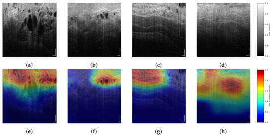
Figure 5.
(Best viewed in color) Several VLE frames and its corresponding class activation maps (CAM). Images (a,b) belong to regions of interest (ROIs) with high-grade dysplasia (HGD), represented as class activation map (CAM) in images (e,f). Images (c,d) correspond to ROIs with non-dysplastic Barrett’s esopaghagus (NDBE), with its CAM in images (g,h). Scale bars: 0.5 mm. Color bar (a–d): pixel intensity. Color bar (e–h): class activation intensity.
Table 3 shows the differences between the reported studies. In comparison with Swager et al. [14], and similar to Scheeve et al. [15], we have obtained a dataset of in-vivo VLE images, but with the following differences: (1) our dataset is different from Swager et al. but closer to Scheeve et al. and (2) our dataset is larger than the other two references (Scheeve et al. compares only 18 patients). Our work improves in both the data acquistion and the evaluation method, by using a dataset of 22 in-vivo patients to uniquely train three DCNNs and further evaluate the results in a separate set of 23 in-vivo unseen patients. We use the AUC as the comparison metric because it is the most suitable value that better quantifies the work done in the aforementioned studies. Our work shows that we achieve the best reported results by utilizing a larger dataset in combination with state-of-the-art DCNNs. Moreover, in comparison with previous studies we take advantage of adjacent VLE frames to improve the classification results for a more robust prediction of neoplasia. Although our results are a positive step towards VLE interpretation, we have the opinion that an even larger dataset will provide more insight into understanding VLE and will pave the way towards further improving early detection of EAC.
5. Conclusions
Barrett’s esophagus (BE) is precursor of esophageal cancer, where detection of neoplasia in patients with this condition can enable early prevention and avoid further complications. We show that deep convolutional neural networks are capable of classifying a VLE region of interest between non-dysplastic BE (NDBE) and high-grade dysplasia (HGD). In this work we have trained several DCNNs to classify neoplasia in patients with BE and we evaluated them in a dataset of 45 patients. We obtained a specificity of , a sensitivity of and an AUC of on the test dataset, which clearly outperforms earlier work. Compared to earlier work, we took advantage of multi-frames of the in-vivo endoscopic acquistion to improve the confidence of our algorithm on predicting neoplasia. As far as our knowledge extends, our work is the first to train DCNNs on in-vivo VLE images and validate it using an unseen dataset. In our opinion, the presented study will improve the treatment of patients with BE by providing assistance to endoscopists. Our work could potentially aid clinicians towards a more accurate localization of regions of interest during biopsy extraction and provide an assessment to replace costly histopathological examinations.
Author Contributions
Conceptualization, R.F., T.S. and F.v.d.S.; methodology, R.F. and T.S.; software, R.F., T.S. and F.v.d.S.; validation, R.F. and T.S.; formal analysis, R.F and T.S; investigation, M.R.S. and A.J.d.G.; resources, W.L.C., E.J.S., J.J.G.H.M.B. and P.H.N.d.W.; data curation, M.R.S., A.J.d.G., W.L.C., E.J.S. and J.J.G.H.M.B.; writing—original draft preparation, R.F. and T.S.; writing—review and editing, F.v.d.S. and P.H.N.d.W.; visualization, R.F. and T.S.; supervision, F.v.d.S., J.J.G.H.M.B. and P.H.N.d.W.; project administration, F.v.d.S., J.J.G.H.M.B. and P.H.N.d.W.; funding acquisition, J.J.G.H.M.B. and P.H.N.d.W.
Funding
This project has received funding from the European Union Research and Innovation Programme Horizon 2020 (H2020/2014–2020) under the Marie Skłodowska-Curie grant agreement No. 721766 (FBI Project). The collaboration project is financed by the Ministry of Economic Affairs of the Netherlands by means of the PPP Allowance made available by the Top Sector Life Sciences and Health to Amsterdam UMC to stimulate public-private partnerships.
Acknowledgments
We gratefully acknowledge the collaboration of NinePoint Medical, Inc. and David Vader. We gratefully acknowledge the support of NVIDIA Corporation with the donation of the Titan Xp GPU used for this research.
Conflicts of Interest
Amsterdam UMC received funding from NinePoint Medical, Inc. for an investigator initiated study of VLE guided laser marking in Barrett’s esophagus. Amsterdam UMC and Eindhoven University of Technology received research funding from NinePoint Medical, Inc. for developing a computer assisted detection tool for VLE on which NinePoint Medical, Inc. holds the intellectual property.
References
- Arnold, M.; Laversanne, M.; Brown, L.M.; Devesa, S.S.; Bray, F. Predicting the Future Burden of Esophageal Cancer by Histological Subtype: International Trends in Incidence up to 2030. Am. J. Gastroenterol. 2017, 112, 1247–1255. [Google Scholar] [CrossRef] [PubMed]
- Zhang, Y. Epidemiology of esophageal cancer. World J. Gastroenterol. 2013, 19, 5598–5606. [Google Scholar] [CrossRef] [PubMed]
- Tschanz, E.R. Do 40% of Patients Resected for Barrett Esophagus With High-Grade Dysplasia Have Unsuspected Adenocarcinoma? Arch. Pathol. Lab. Med. 2005, 129, 177–180. [Google Scholar] [CrossRef] [PubMed]
- Gordon, L.G.; Mayne, G.C.; Hirst, N.G.; Bright, T.; Whiteman, D.C.; Watson, D.I. Cost-effectiveness of endoscopic surveillance of non-dysplastic Barrett’s esophagus. Gastrointest. Endosc. 2014, 79, 242–256.e6. [Google Scholar] [CrossRef]
- Schölvinck, D.W.; van der Meulen, K.; Bergman, J.J.G.H.M.; Weusten, B.L.A.M. Detection of lesions in dysplastic Barrett’s esophagus by community and expert endoscopists. Endoscopy 2017, 49, 113–120. [Google Scholar] [CrossRef]
- Leggett, C.L.; Gorospe, E.C.; Chan, D.K.; Muppa, P.; Owens, V.; Smyrk, T.C.; Anderson, M.; Lutzke, L.S.; Tearney, G.; Wang, K.K. Comparative diagnostic performance of volumetric laser endomicroscopy and confocal laser endomicroscopy in the detection of dysplasia associated with Barrett’s esophagus. Gastrointest. Endosc. 2016, 83, 880–888.e2. [Google Scholar] [CrossRef] [PubMed]
- Swager, A.F.; Tearney, G.J.; Leggett, C.L.; van Oijen, M.G.; Meijer, S.L.; Weusten, B.L.; Curvers, W.L.; Bergman, J.J. Identification of volumetric laser endomicroscopy features predictive for early neoplasia in Barrett’s esophagus using high-quality histological correlation. Gastrointest. Endosc. 2017, 85, 918–926.e7. [Google Scholar] [CrossRef]
- Swager, A.F.; van Oijen, M.G.; Tearney, G.J.; Leggett, C.L.; Meijer, S.L.; Bergman, J.J.G.H.M.; Curvers, W.L. How Good are Experts in Identifying Early Barrett’s Neoplasia in Endoscopic Resection Specimens Using Volumetric Laser Endomicroscopy? Gastroenterology 2016, 150, S628. [Google Scholar] [CrossRef]
- Swager, A.F.; van Oijen, M.G.; Tearney, G.J.; Leggett, C.L.; Meijer, S.L.; Bergman, J.J.G.H.M.; Curvers, W.L. How Good Are Experts in Identifying Endoscopically Visible Early Barrett’s Neoplasia on in vivo Volumetric Laser Endomicroscopy? Gastrointest. Endosc. 2016, 83, AB573. [Google Scholar] [CrossRef]
- van der Sommen, F.; Zinger, S.; Curvers, W.L.; Bisschops, R.; Pech, O.; Weusten, B.L.A.M.; Bergman, J.J.G.H.M.; de With, P.H.N.; Schoon, E.J. Computer-aided detection of early neoplastic lesions in Barrett’s esophagus. Endoscopy 2016, 48, 617–624. [Google Scholar] [CrossRef] [PubMed]
- Qi, X.; Sivak, M.V.; Isenberg, G.; Willis, J.; Rollins, A.M. Computer-aided diagnosis of dysplasia in Barrett’s esophagus using endoscopic optical coherence tomography. J. Biomed. Opt. 2006, 11, 1–10. [Google Scholar] [CrossRef]
- Qi, X.; Pan, Y.; Sivak, M.V.; Willis, J.E.; Isenberg, G.; Rollins, A.M. Image analysis for classification of dysplasia in Barrett’s esophagus using endoscopic optical coherence tomography. Biomed. Opt. Express 2010, 1, 825–847. [Google Scholar] [CrossRef]
- Ughi, G.J.; Gora, M.J.; Swager, A.F.; Soomro, A.; Grant, C.; Tiernan, A.; Rosenberg, M.; Sauk, J.S.; Nishioka, N.S.; Tearney, G.J. Automated segmentation and characterization of esophageal wall in vivo by tethered capsule optical coherence tomography endomicroscopy. Biomed. Opt. Express 2016, 7, 409–419. [Google Scholar] [CrossRef] [PubMed]
- Swager, A.F.; van der Sommen, F.; Klomp, S.R.; Zinger, S.; Meijer, S.L.; Schoon, E.J.; Bergman, J.J.; de With, P.H.; Curvers, W.L. Computer-aided detection of early Barrett’s neoplasia using volumetric laser endomicroscopy. Gastrointest. Endosc. 2017, 86, 839–846. [Google Scholar] [CrossRef] [PubMed]
- Scheeve, T.; Struyvenberg, M.R.; Curvers, W.L.; de Groof, A.J.; Schoon, E.J.; Bergman, J.J.G.H.M.; van der Sommen, F.; de With, P.H.N. A novel clinical gland feature for detection of early Barrett’s neoplasia using volumetric laser endomicroscopy. In Proceedings of the Medical Imaging 2019: Computer-Aided Diagnosis, San Diego, CA, USA, 13 March 2019; Mori, K., Hahn, H.K., Eds.; International Society for Optics and Photonics: Bellingham, WA, USA, 2019; Volume 10950, p. 109501Y. [Google Scholar] [CrossRef]
- Yun, S.H.; Tearney, G.J.; de Boer, J.F.; Iftimia, N.; Bouma, B.E. High-speed optical frequency-domain imaging. Opt. Express 2003, 11, 2953–2963. [Google Scholar] [CrossRef]
- Yun, S.H.; Tearney, G.J.; Vakoc, B.J.; Shishkov, M.; Oh, W.Y.; Desjardins, A.E.; Suter, M.J.; Chan, R.C.; Evans, J.A.; Jang, I.K.; Nishioka, N.S.; de Boer, J.F.; Bouma, B.E. Comprehensive volumetric optical microscopy in vivo. Nat. Med. 2006, 12, 1429–1433. [Google Scholar] [CrossRef]
- Vakoc, B.J.; Shishko, M.; Yun, S.H.; Oh, W.Y.; Suter, M.J.; Desjardins, A.E.; Evans, J.A.; Nishioka, N.S.; Tearney, G.J.; Bouma, B.E. Comprehensive esophageal microscopy by using optical frequency–domain imaging (with video). Gastrointest. Endosc. 2007, 65, 898–905. [Google Scholar] [CrossRef]
- Suter, M.J.; Vakoc, B.J.; Yachimski, P.S.; Shishkov, M.; Lauwers, G.Y.; Mino-Kenudson, M.; Bouma, B.E.; Nishioka, N.S.; Tearney, G.J. Comprehensive microscopy of the esophagus in human patients with optical frequency domain imaging. Gastrointest. Endosc. 2008, 68, 745–753. [Google Scholar] [CrossRef]
- Levine, D.S.; Haggitt, R.C.; Blount, P.L.; Rabinovitch, P.S.; Rusch, V.W.; Reid, B.J. An endoscopic biopsy protocol can differentiate high-grade dysplasia from early adenocarcinoma in Barrett’s esophagus. Gastroenterology 1993, 105, 40–50. [Google Scholar] [CrossRef]
- Shaheen, N.J.; Falk, G.W.; Iyer, P.G.; Gerson, L.B. ACG Clinical Guideline: Diagnosis and Management of Barrett’s Esophagus. Am. J. Gastroenterol. 2016, 111, 30–50. [Google Scholar] [CrossRef]
- Swager, A.F.; de Groof, A.J.; Meijer, S.L.; Weusten, B.L.; Curvers, W.L.; Bergman, J.J. Feasibility of laser marking in Barrett’s esophagus with volumetric laser endomicroscopy: first-in-man pilot study. Gastrointest. Endosc. 2017, 86, 464–472. [Google Scholar] [CrossRef]
- Klomp, S.; Sommen, F.v.d.; Swager, A.F.; Zinger, S.; Schoon, E.J.; Curvers, W.L.; Bergman, J.J.G.H.M.; de With, P.H.N. Evaluation of image features and classification methods for Barrett’s cancer detection using VLE imaging. In Proceedings of the Medical Imaging 2017: Computer-Aided Diagnosis, Orlando, FL, USA, 3 March 2017; Armato, S.G., Petrick, N.A., Eds.; International Society for Optics and Photonics: Bellingham, WA, USA, 2017; Volume 10134, p. 101340D. [Google Scholar] [CrossRef]
- van der Sommen, F.; Klomp, S.R.; Swager, A.F.; Zinger, S.; Curvers, W.L.; Bergman, J.J.G.H.M.; Schoon, E.J.; de With, P.H.N. Predictive features for early cancer detection in Barrett’s esophagus using volumetric laser endomicroscopy. Comput. Med. Imaging Graph. 2018, 67, 9–20. [Google Scholar] [CrossRef] [PubMed]
- van der Putten, J.; van der Sommen, F.; Struyvenberg, M.; de Groof, J.; Curvers, W.; Schoon, E.; Bergman, J.G.H.M.; de With, P.H.N. Tissue segmentation in volumetric laser endomicroscopy data using FusionNet and a domain-specific loss function. In Proceedings of the Medical Imaging 2019: Image Processing, San Diego, CA, USA, 15 March 2019; Angelini, E.D., Landman, B.A., Eds.; International Society for Optics and Photonics: Bellingham, WA, USA, 2019; Volume 10949, p. 109492J. [Google Scholar] [CrossRef]
- Jain, S.; Dhingra, S. Pathology of esophageal cancer and Barrett’s esophagus. Ann. Cardiothorac. Surg. 2017, 6, 99–109. [Google Scholar] [CrossRef]
- Fang, L.; Cunefare, D.; Wang, C.; Guymer, R.H.; Li, S.; Farsiu, S. Automatic segmentation of nine retinal layer boundaries in OCT images of non-exudative AMD patients using deep learning and graph search. Biomed. Opt. Express 2017, 8, 2732–2744. [Google Scholar] [CrossRef] [PubMed]
- Lee, C.S.; Tyring, A.J.; Deruyter, N.P.; Wu, Y.; Rokem, A.; Lee, A.Y. Deep-learning based, automated segmentation of macular edema in optical coherence tomography. Biomed. Opt. Express 2017, 8, 3440–3448. [Google Scholar] [CrossRef] [PubMed]
- Schlegl, T.; Waldstein, S.M.; Bogunovic, H.; Endstraßer, F.; Sadeghipour, A.; Philip, A.M.; Podkowinski, D.; Gerendas, B.S.; Langs, G.; Schmidt-Erfurth, U. Fully Automated Detection and Quantification of Macular Fluid in OCT Using Deep Learning. Ophthalmology 2018, 125, 549–558. [Google Scholar] [CrossRef] [PubMed]
- Lee, C.S.; Baughman, D.M.; Lee, A.Y. Deep Learning Is Effective for Classifying Normal versus Age-Related Macular Degeneration OCT Images. Kidney Int. Rep. 2017, 2, 322–327. [Google Scholar] [CrossRef]
- Prahs, P.; Radeck, V.; Mayer, C.; Cvetkov, Y.; Cvetkova, N.; Helbig, H.; Märker, D. OCT-based deep learning algorithm for the evaluation of treatment indication with anti-vascular endothelial growth factor medications. Graefe’s Arch. Clin. Exp. Ophthalmol. 2018, 256, 91–98. [Google Scholar] [CrossRef] [PubMed]
- Russakovsky, O.; Deng, J.; Su, H.; Krause, J.; Satheesh, S.; Ma, S.; Huang, Z.; Karpathy, A.; Khosla, A.; Bernstein, M.; Berg, A.C.; Fei-Fei, L. ImageNet Large Scale Visual Recognition Challenge. Int. J. Comput. Vis. 2015, 115, 211–252. [Google Scholar] [CrossRef]
- Simonyan, K.; Zisserman, A. Very Deep Convolutional Networks for Large-Scale Image Recognition. arXiv 2014, arXiv:1409.1556. [Google Scholar]
- Zhou, B.; Khosla, A.; Lapedriza, A.; Oliva, A.; Torralba, A. Learning Deep Features for Discriminative Localization. In Proceedings of the 2016 IEEE Conference on Computer Vision and Pattern Recognition (CVPR), Las Vegas, Nevada, 27–30 June 2016. [Google Scholar] [CrossRef]
- Wang, Z.; Lee, H.C.; Ahsen, O.; Liang, K.; Figueiredo, M.; Huang, Q.; Fujimoto, J.; Mashimo, H. Computer-Aided Analysis of Gland-Like Subsurface Hyposcattering Structures in Barrett’s Esophagus Using Optical Coherence Tomography. Appl. Sci. 2018, 8, 2420. [Google Scholar] [CrossRef]
© 2019 by the authors. Licensee MDPI, Basel, Switzerland. This article is an open access article distributed under the terms and conditions of the Creative Commons Attribution (CC BY) license (http://creativecommons.org/licenses/by/4.0/).