Energy Demand and Supply Simultaneous Optimization to Design a Nearly Zero-Energy House

Featured Application

The results of this paper can support the design of nearly zero-energy single-family houses in the Italian context. The provided methodological framework can support the design of nearly zero-energy buildings and be replicated in different contexts.

Abstract

The effective design of nearly zero-energy buildings depends on a large set of interdependent variables, which affect both energy demand and supply. Considering them simultaneously is fundamental when searching for optimal design of nearly zero-energy buildings, as encouraged by the EU in the second recast of the Energy Performance of Building Directive (EPBD). This paper presents the application of the new energy demand and supply simultaneous optimization (EDeSSOpt) methodology to optimize the design of a single-family house in the Italian context. Both primary energy optimization and financial optimization are carried out in the context of European regulations. Robustness of the resulting optimal solution is studied through analysis of optimum neighborhoods. The resulting cost-optimized solution relies on a moderately insulated envelope, a highly efficient system, and 34% of coverage from renewables. The energy-optimized solution requires a higher level of insulation and a higher coverage from renewables, demonstrating that there is still a gap between energy and cost optimums. Beyond the results, integrated optimization by means of EDeSSOpt is demonstrated to better minimize cost functions while improving the robustness of results.

1. Introduction

It is broadly acknowledged that the building sector is responsible for a considerable fraction of energy consumption and CO₂ emissions that can be attributed to a nation. In Europe, these percentages are approximately 40% (primary energy consumption) and 36% (CO₂ emissions) of the annual overall energy outlay and greenhouse gas emissions. As a result, the building sector has been identified as one of the key areas in which measures have to be taken in order to achieve the 20/20/20 targets (20% of greenhouse gas emissions compared to 1990, 20% energy savings by 2020, compared to a business scenario, and 20% share of renewables in 2020) that the Member States have set by common agreement [1].

From this perspective, the first recast of the Energy Performance of Building Directive (EPBD) established the framework and the limits to fulfill these targets. They impose an adoption of measures to improve energy efficiency in buildings in order to satisfy the requirement where, by 31 December 2020, all new buildings should be nearly zero-energy buildings (NZEBs), which are defined as “buildings whose energy requirement should be very low and significantly covered by renewable energy sources” [2]. The second recast of EPBD further encourages NZEB design towards the medium-term target of reducing greenhouse gas emissions 88–91% by 2050 (compared to 1990) [3].

Furthermore, it is recognized that these objectives cannot be pursued without considering financial feasibility, considering that improving the energy performance of buildings is one of the measures with the largest potential for net economic savings in all building types [4,5]. In this respect, EU established a comparative methodology framework to compare different design alternatives under a cost-optimal perspective [6].

This approach has acted as one of the main drivers for the European scientific community to carry out research related to NZEB design [7]. Many studies performed across Europe demonstrate that efficient NZEB design results from optimal interactions between the many variables impacting energy demand (mainly related to the building envelope), energy supply (related to systems and renewables), and the technical and economic scenarios in which the building is designed. That is why the design of NZEBs can be identified as a complex optimization problem. Considering the complexity of such a problem, growing interest has been reserved to computer-based optimization techniques throughout building research communities [8]. These techniques, also known as simulation-based optimization methods (SBOMs), are based on the combination of a building dynamic energy simulation program and an optimization engine, and they consist of an iterative calculation process performed using a computer-automated model driven by a specific optimization algorithm [9].

Reasons for the success of SBOM are seen in its relatively less expensive design and quicker computation time; this is because of the larger, faster, and therefore more efficient exploration of the design space. That is why SBOM appears to be the most promising method to search for NZEB optimal solutions with the greatest exploration of the design space while maintaining manageable calculations.

From a review of recent applications of computational optimization methods applied to building design [10], the design variables that typically affect energy demand are:

• the shape of the building and its orientation;
• the thermal insulation and inertia of the opaque and transparent envelope;
• the type and size of possible devices to control solar radiation; and
• the optical properties of the transparent elements.

Regarding the energy supply side, the following variables may be considered:

• the type and number of energy generator/converters as well as their sizing;
• the type and size of heating and cooling terminals in thermal zones; and
• the presence and sizing of thermal storages or electrical storage batteries.

In addition to this, the boundary conditions and input data listed below have to be considered:

• the weather conditions;
• the occupants’ usage profile;
• the indoor environmental requirements; and
• the optimization criteria.

In the literature, considering the techno-economic objective of NZEB design, many studies focus on variables that minimize the building’s energy demand [11,12,13,14], while many others focus on maximizing the energy supply [15,16,17]. However, the interdependence between energy supply and demand has been demonstrated [18,19,20,21,22].

To consider this interdependence and allow a whole NZEB optimization process to be carried out, a new methodology was introduced and was firstly applied to the optimization of a multifamily building in the Italian context [23]. However, further applications are needed to refine the methodology and get results for other building typologies.

Concerning nearly zero-energy single-family houses, some examples can be found in the Italian context [24,25], demonstrating that it is possible to reach the NZEB target in a Mediterranean climate [26]. However, detailed and integrated optimization studies could be performed to further investigate whether it is possible to reach better performances while ensuring the cost-effectiveness of the resulting design solutions and also consider the future development of energy use in residential buildings [27]. In this perspective, Barthelmes et al. [28] analyzed a single-family house located in the Piedmont Region (North Italy) in terms of architectural design, economic constrains, and energy performances by optimizing both variables related to energy demand and supply. Calculations of energy consumptions are performed by means of a dynamic energy simulation, but automated optimization is not implemented, which leaves the optimization process to a manual comparison of a few alternatives.

Objective and Approach

Given the current state, the objective of this work was to optimize the design of a nearly zero-energy single-family house in Northern Italy by means of energy supply and demand simultaneous optimization (EDeSSOpt). Further, the paper analyzed the potential differences in the building envelope and systems design resulting from the use of an integrated (rather than a sequential) simulation-based optimization method. In detail, the study aimed at:

-

identifying the key design variables affecting both energy demand and supply and defining the related costs;

-

tailoring the simulation-based optimization methodology to the so-defined optimization problem;

-

carrying out sequential optimization (envelope optimization first, then systems and RES optimizations) for both financial and energy objectives;

-

performing EDeSSOpt optimization for both energy and financial objectives;

-

evaluating the robustness of results by analyzing the optimum neighborhood; and

-

comparing results obtained from the application of the sequential approach and from the EDeSSOpt method.

2. Materials and Methods

2.1. Energy Demand and Supply Simultaneous Optimization (EDeSSOpt) Methodology

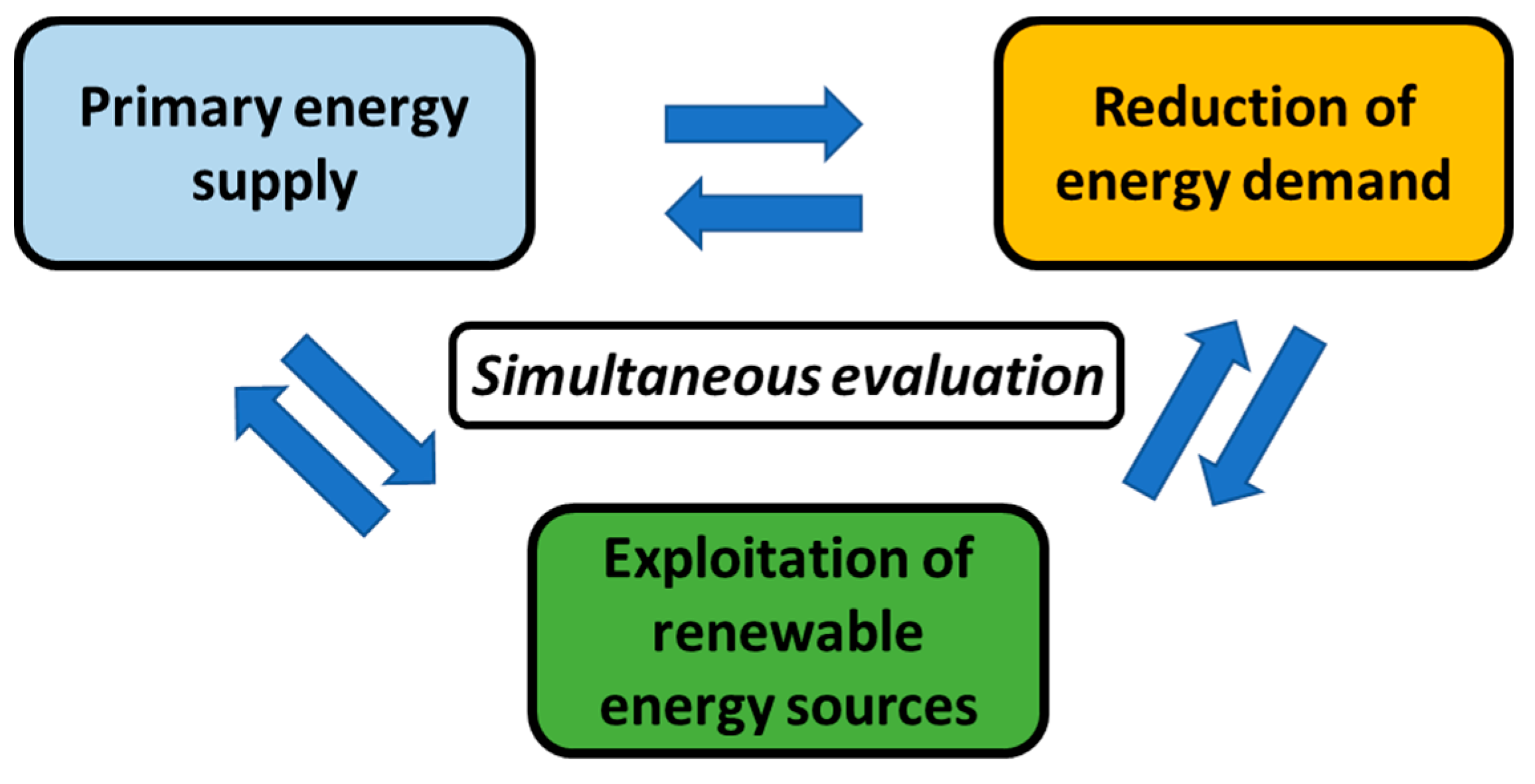
The methodology used in the present study consisted of the simultaneous assessment and optimization of energy demand and supply (Figure 1) of a single-family NZEB.

The so-called EDeSSOpt methodology, described in detail in [23], can be summarized in three main phases.

In the preprocessing phase, the design variables (termed decision parameters) are defined in relation to the building envelope, the systems, and renewable energy technologies. Further, the energy model is set up. In this work, the energy model was created in TRNSYS^® (Transient System Simulation Tool).

In the optimization phase, the optimization algorithm is set, and the GenOpt^® (Generic Optimization Program) optimizer is coupled with the simulation model. The optimization process is run to minimize a defined objective function. In this work, the global cost as well as the total and nonrenewable primary energy objective functions were minimized.

In the postprocessing phase, the obtained results are analyzed in terms of both the exploration of the design space and the analysis of the optimal solution. An analysis in the neighborhood of optimal solutions was performed to assess their robustness. Figure 2 helps to better understand the main phases of the integrated simulation-based optimization method that was used for this study.

2.2. The Case Study Building

The case study building was represented by a reference layout for a single-family house located in Turin, Northern Italy. According to the Italian legislation, this city is included in the “E” thermal zone, meaning that the temperature for the design heat load is equal to −8 °C, and that the number of heating degree-days (HDDs) can range from a minimum of 2100 to a maximum of 3000.

The building consisted of two floors, and it had a net internal floor area of 155 m². A kitchen, a large living room, one bedroom, and one bathroom were on the ground floor, while two bedrooms, a working/relaxing space, and a bathroom composed the first floor.

Concerning the reference building envelope, the external walls were made up of brick blocks, and the structure was a concrete frame type. The pitched roof had a surface of nearly 70 m² with a major proportion of it (about 60%) being south-oriented and, therefore, ideal for the installation of solar energy renewable sources. To maximize solar gains, the majority of the large glass openings were located on the south-oriented walls, with the overall window area being approximately one-fifth of the gross floor area. To avoid the risk of overheating during the summer season, shading overhangs protected the openings without nullifying the beneficial effects during the winter season.

Concerning the systems, a reference configuration was considered for the initial scenario according to current Italian legislation [29]. The system for space heating and domestic hot water (DHW) was a gas condensing boiler. The cooling equipment was represented by an electric chiller. Reference values of generation, distribution, and emission efficiencies were also considered in accordance with current legislation. Each room had a different thermal zone with a different occupancy profile and an independent HVAC system control.

2.3. Decision Parameters

A comparative evaluation of different design alternatives had to be performed in order to find an optimal solution to the NZEB design problem. To do so, system and building envelope technical solutions (other than the reference ones) were identified as decision parameters. Each parameter should refer to a different design variable and should vary in a range that was properly set to ensure technical feasibility. The step of variation, that is the number of intervals in which the optimization range is divided into, should also reflect the real availability on the market of each design solution.

Table 1. Passive decision parameters (building envelope) and related variability range.

Name	Decision Parameter	Unit	Variability Range
			Min	Max	# Step
ResO	Thermal resistance of the outwall insulation	[m2K/W]	0.9	18	10
TO	Thickness of the outwall massive layers	[m]	0.1	0.4	2
ResR	Thermal resistance of the roof insulation	[m2K/W]	0.9	18	10
ResS	Thermal resistance of the slab insulation	[m2K/W]	0.9	18	10
WT	Vertical window types	[-]	Three options (1, 2, 3—Table 2)
RWT	Roof window types	[-]	One option (4—Table 2)
GWW	Ground floor window width (south, height = 2.15 m)	[m]	2.2	7.8	20
FWW	First floor window width (south, height = 0.8 m)	[m]	0.2	7.8	15
RWH	Roof window height (width = 2.3 m)	[m]	0	4.8	4

reports envelope-related parameters, also denoted as passive decision parameters because their variation may impact building energy performance through reducing building energy needs.

The window type was an optimization variable whose values stood for the most common types of windows that could be found in the Italian construction market. The meaning of each parameter value is clarified in

Table 2. Description of window types for parameters WT and RWT.

Window Type	Description	Ug [W/m2K]	g-Value
1	4/15/4—Double glazing with air	2.8	0.70
2	4/15/4—Double glazing, low-emissive (low-e), with Argon	1.6	0.58
3	4/12/4/12/4—Triple glazing, low-e, with air	1.2	0.50
4	4/12/4/12/4—Triple glazing, low-e, with Argon	1	0.40

.

With reference to the solar thermal system, as reported in

Table 3. Active decision parameters (systems) and related variability range.

	Decision Parameter	Unit	Variability Range
			Min	Max	Step
N_coll	Number of solar thermal collectors	[-]	2	14	2
Slope_coll	Slope of solar thermal collectors	[°]	18	45	15
St_ratio	Ratio between storage volume and collector surface	[L/m2]	50	100	25
Type_coll	Type of solar thermal collector	[-]	Choice between two options
Type_PV	Type of PV panel	[-]	Choice between three options
Slope_PV	Slope of PV panels	[°]	18	45	15
N_PV	Number of PV panels	[-]	2	18	2
Type_heat	Heating type	[-]	Choice between two options

, the selected decision parameters were related to the technology type (flat plate or evacuated tube collectors); the surface, orientation, and slope of the collectors; and the ratio between the surface of the installed solar collectors and the volume of the storage tank/puffer. Similarly, decision parameters related to the photovoltaic system (PV) referred to the type (monocrystalline, polycrystalline, and amorphous silicon), surface, orientation, and slope of the installed PV panels. Another decision parameter controlled the heating type (gas condensing boiler or geothermal heat pump).

The entire set of system-related decision parameters is reported in Table 3.

The variability range was expressed by means of the upper and lower limits of the interval that was divided in a defined number of steps. These settings were based on the analysis of currently available typical products on the Italian market. Since the present study focused on the optimization of building constructive elements and systems, investigation of variables in continuous space did not make sense because the market offered only some measures and dimensions, thus handling discrete values expressed through the number of steps.

Considering a single collector area of 2 m², the maximum number of solar thermal collectors was set to 14 since the correspondent surface was equal to 30 m², which was approximately half the surface of the south-oriented pitched roof (on the assumption that the total available surface was equally shared between the solar thermal and PV systems). For the same reason, the maximum number of PV panels was equal to 18, considering a single PV panel area of 1.6 m².

2.4. Simulation for Optimization

In order to perform the desired optimization study, the simulation model should be properly designed since its first conception.

First, it was necessary to create a “customized” weather file. The basis for such an operation was the weather file for the reference location, which was then modified by adding winter and summer design days before the start of the entire year of simulation. This enabled us to calculate, before starting each simulation, the design capacities and the flowrate based on the actual heating and cooling needs. In this way, system sizing and pricing can be properly performed at each iteration of the optimization process based on the required heating and cooling capacity, which results from the selected set of parameter values for a building design configuration.

Then, all system alternatives were included in the same model, and a control center was created to control the entire set of components included in the system design option, which was selected from the optimization algorithm at each iteration.

2.5. Optimization Algorithm

To carry out the optimization process, a binary version of the particle swarm optimization algorithm [30] was chosen as the optimization algorithm to use given its robustness and efficiency in converging towards the global minimum in problems with discrete variables [31]. It has also demonstrated to be effective when applied to building optimization studies [32].

The schematic for the optimization process is pictured in Figure 3. As shown, GenOpt assigned a set of parameter values at each iteration that were then entered to TRNSYS, which performed the energy simulation and calculated the value of the objective function. Based on the so-calculated value of the objective function and the updated equations of the optimization algorithm, another set of values to be assigned to the parameters was selected in order to perform a new simulation and a new objective function calculation. This iterative cycle ended when the maximum number of generations was reached. GenOpt then registered the value assumed by each of the optimization variables at each run together with the correspondent objective function value until convergence.

2.6. Objective Functions

2.6.1. Financial Objective

Financial calculations were carried out according to the global cost method, which was described in the European Standard EN 15459 [33]. This standard presented a calculation method for the costs of all systems involved in the energy demand and consumption of a building. Therefore, it was used to compare different energy systems and building configurations with regard to the associated global cost, which can be evaluated by summing up the initial investment costs together with periodic, replacement, and annual costs as well as adding energy costs referred to in the duration of the calculation. In the end, final value had to be subtracted from the calculated amount. All costs, except for the initial investment costs, had to be referred to the starting year of calculation.

In view of the above, the financial objective function can be written as follows:

$$C_G\left(\tau \right)=CI+{{\displaystyle \sum }}_J\left[{{\displaystyle \sum }}_{i=1}^{\tau }\left(C_{a,i}\left(j\right)\cdot R_d\left(i\right)\right)-V_{f,\tau }\left(j\right)\right],$$

(1)

where:

• $C_G\left(\tau \right)$ represents the global cost referred to a starting year ${\tau }_0$;
• $CI$ stands for the initial investment cost;
• $C_{a,i}\left(j\right)$ is the annual cost for component j at the year i;
• $R_d\left(i\right)$ represents the discount rate for the year i; and
• $V_{f,\tau }\left(j\right)$ is the final value of component j at the end of the calculation period.

According to the guidelines issued with the 2010/31/UE directive [6], the calculation period was set to 30 years, and the real interest rate was set to 4%. (Refer to [7] for details about the calculation assumptions.)

2.6.2. Energy Objective

The energy objective was set in terms of primary energy. In particular, two objective functions were defined, one referring to nonrenewable primary energy for heating and cooling (Equation (2)) and the other referring to the total primary energy for heating and cooling (Equation (3)).

$$P{E}_{nren}=P{E}_{H,nren}+P{E}_{C,nren}.$$

(2)

$$P{E}_{tot}=P{E}_{H,tot}+P{E}_{C,tot}.$$

(3)

The primary energy conversion factors were set according to Italian regulation [29].

In detail, they were set to:

• 1.95—nonrenewable primary energy conversion factor for electricity;
• 2.42—total primary energy conversion factor for electricity;
• 1.05—nonrenewable/total primary energy conversion factor for natural gas (natural gas is nonrenewable);
• 1—renewable/total primary energy conversion factor for thermal and electrical energy generated from solar thermal and PV, respectively (these sources are renewable).

3. Results

As mentioned, one of the aims of the present study was to investigate how and to what extent an integrated (simulation-based) approach, compared to a sequential (optimization) process, affected the cost-effective design of a nearly zero-energy house. Therefore, in this section, results related to the two-step sequential optimization were firstly presented (energy demand first, energy supply second), followed by the integrated optimization carried out with the EDeSSOpt method. Since such financial optimization was carried out according to EU methodology for NZEB design, results were analyzed according to the following principles:

• the financial optimum is provided by the package corresponding to the lowest global cost;
• at the same cost-level, the package with the lower energy consumption should be selected; and
• all the selected packages should be assessed with respect to their financial and environmental impacts.

Furthermore, results related to integrated optimization carried out with the energy objective were presented in order to compare a global, cost-driven optimization process to a primary energy-driven optimization and to better quantify their environmental impact.

Table 4. Summary of optimization runs and sections for results presentation.

	Approach
	Sequential		Integrated
Objective	Demand	Supply	Demand + Supply
Financial (Equation (1))	Section 3.1	Section 3.2	Section 3.3
Energy (Equation (3))			Section 3.4

provides a summary of the performed optimization runs and the related section in which results are presented.

Considering that running the TRNSYS model of the case study took about 2 min (Intel^® Core™ i7-4770, 3.4 GHz, 8 MB cache, 4 core, HD 4600), and that eight simulations could be performed in parallel, the computation time for each optimization process depended on the number of different design options explored within the same run. For a given number of iterations (1500), the maximum computation time was 6 h and 15 min for each optimization process.

3.1. Financial Objective—Sequential Optimization and Energy Demand

Results in this section refer to the minimization of the global cost objective function (Equation (1)) considering the variation of passive decision parameters (Table 1 and Table 2).

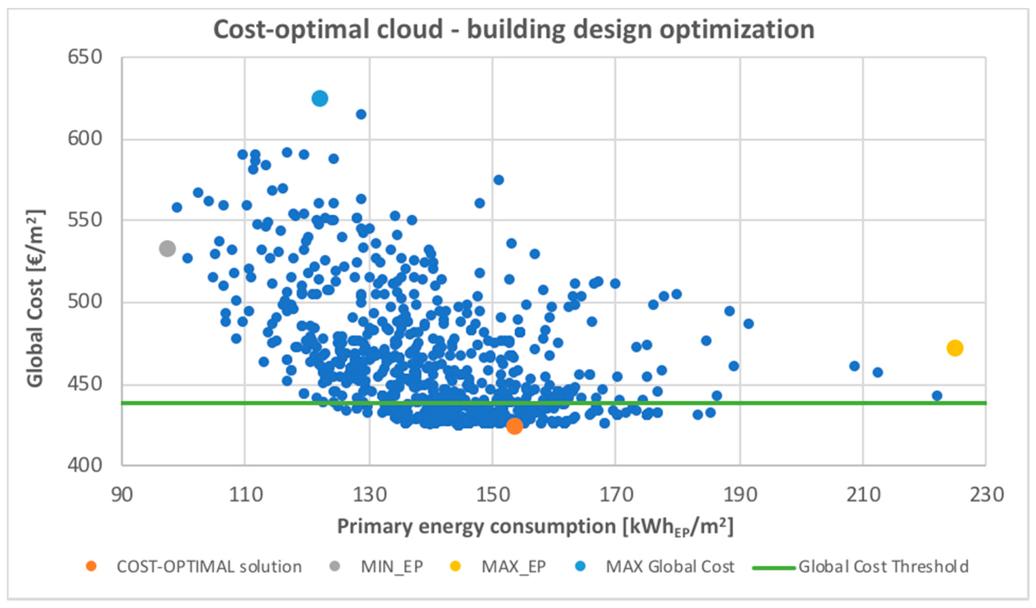
Overall, almost 700 iterations were performed, each leading to simulate a different design alternative. The entire set of design alternatives that were analyzed within this optimization process were reported in a cost-optimal diagram in Figure 4, where the global cost objective function was reported on the vertical axis, and the total primary energy was reported on the horizontal axis. To compute the primary energy associated to each design alternative, a baseline reference energy system was considered in accordance with the guidelines issued on this subject by Italian regulation [24].

As shown, the global cost ranged between 626 €/m² and 424 €/m², while the related total primary energy ranged between 97 kWh/m² and 225 kWh/m².

The resulting cost optimal design, indicated by the orange point in Figure 4, referred to a nonrenewable primary energy of 154 kWh/m² for the minimum global cost of 424 €/m². In the same graph, other significant points were highlighted: the grey point indicated the solution with the lowest primary energy, the light blue point referred to the highest evaluated global cost, while the yellow point indicated the highest primary energy value. The values of parameters defining the design alternatives represented by these points are reported in

Table 5. Values of parameters of the resulting cost-optimal point and of other significant points.

	Parameter	Unit	COST-OPTIMAL	MIN_EP	MAX_EP	MAX Global Cost
Building Parameters	Thermal resistance of the outwall insulation	[m2K/W]	2.7	12.6	0.9	16.2
	Thickness of the outwall massive layers	[m]	0.1	0.5	0.1	0.3
	Thermal resistance of the roof insulation	[m2K/W]	1.8	13.5	0.9	16.2
	Thermal resistance of the slab insulation	[m2K/W]	2.7	3	0.9	10.8
	Vertical window type (south façade)	[-]	Double glazing with air
	Vertical window type (east–west–north)	[-]	Triple glazing, low-e with air		Double glazing with air
	Roof window types	[-]	Triple glazing, low-e with Argon
	Ground floor window width (south, height = 2.15 m)	[m]	2.2	2.2	4.6	7.8
	First floor window width (south, height = 0.8 m)	[m]	0.2	0.2	6.2	5.6
	Roof window height (width = 2.3 m)	[m]	0	0	1.2	4.8
Results	Primary energy consumption	[kWhep/m2]	153.61	97.67	225.00	122.06
	Net annual heating demand	[kWh/m2]	89.12	47.14	138.66	50.02
	Net annual cooling demand	[kWh/m2]	6.88	7.56	11.74	29.12
	Net DHW annual demand	[kWh/m2]	14.37	14.37	14.37	14.37
	Gas volume consumption	m3	1762.52	1110.58	2531.83	1155.24

.

In the cost-optimal solution (orange point), optimal design of the opaque envelope was represented by a relatively low thermal resistance for the outwall and slab (corresponding to 9 cm of insulation) and an even thinner insulation layer for the roof (6 cm). In addition to this, the optimal insulation of the outwall was equal to the minimum allowed as well as the thickness of its massive layer. Concerning the transparent envelope, window type 1 (double glazing with air) was selected as optimal for south-oriented openings, of which the dimensions were reduced to their minimum. The highest performing window type (triple glazing, low-emissive with argon) was optimal for other openings.

For this cost-optimal building configuration, the annual heating and cooling demands were equal to 89.12 kWh/m² and 6.88 kWh/m², respectively. This low cooling demand was coherent with the resulting optimal parameter values that were set so that the cooling demand was reduced. As mentioned, the amount of nonrenewable primary energy consumption was quite high (almost 154 kWh/m², according to the primary energy conversion factors provided by the Italian legislation), but it was not surprising, as (in this phase) the modelling of the technical systems was not considered and reference values and efficiencies for systems were used without contributions from renewables.

When comparing the set of resulting cost-optimal values to the other highlighted significant points, high values of insulation, together with high-performance glazing, led to the lowest primary energy consumption, which simultaneously increased the associated global cost, and vice versa. This also emerged from another type of result representation, reported in Figure 5. The grey profiles represented the entire set of evaluated design alternatives, while profiles representing significant points were highlighted in colors.

One of the main advantages of the simulation-based optimization method here adopted was that it was not a deterministic method, providing a single solution as the final output of the whole optimization process, but it allowed exploring the space of the solutions in which it could be possible to find solutions that fit the problem better than the one selected by the optimization algorithm. This was particularly possible in the neighborhood of the resulting optimum, where it was possible to find different design alternatives leading to a very small increase in the objective function with respect to the minimum. In the present study, a 3.5% global cost threshold (green line in Figure 4) was established in order to investigate the solutions included in this neighborhood. Though having a slightly higher global cost, a large number of these points were characterized by a lower primary energy consumption, as reported in Figure 6. In this figure, the grey point stood for the solution (i.e., set of building parameter values) corresponding to the lowest energy consumption within the neighborhood. Despite the associated global cost being increased by 3% (compared to the cost-optimal solution), the primary energy consumption declined by 20% because of the higher thickness of the insulation layer of both the external wall and the slab.

Beyond identification of other possible sets of building design optimization variables leading to a better energy performance, analysis of the neighborhood can provide an interpretation key of the robustness of the optimal solution resulting from the optimization process.

Figure 7 visually represents this statement, as it displays the values of the optimization variables of the solutions inside the neighborhood. The optimal parameter values found by the algorithm were linked together with a red line. The more (blue) lines that converge towards one value, the greater the robustness of the solution. For instance, the optimal value of the variable ‘window type south’ (WTS) appeared in over 80% of the solutions inside the neighborhood, meaning that the resulting optimal value for this parameter was robust. Instead, the optimal value of the roof insulation thickness was selected in just one-third of the cases inside the threshold, indicating that many other design alternatives in the optimum neighborhood were reached with different values of that parameter.

Figure 8 further highlighted this concept, where the frequency of occurrence of each value for the parameter ‘window type south’ (WTS) was reported. In particular, the occurrence of each value within the entire optimization process was pictured in blue, while that referred to the optimum neighborhood was reported in orange. It was clear that double glazing with air was the optimal window type (south orientation) within the explored set, as there was an evident peak in the diagram that described both its absolute and relative frequencies.

3.2. Financial Objective—Sequential Optimization and Energy Supply

The second step of the sequential approach referred to energy supply optimization, entailing financial optimization of active design parameters (Table 3) when the passive ones were fixed to the optimal values resulting from the first step (minimization of energy demand).

The optimization process ran in this second step led to evaluate almost 400 different design options, which were reported in the cost-optimal cloud in Figure 9. The profiles indicating optimal parameter values related to the cost-optimal point and to the other significant points are pictured in Figure 10.

Concerning the solar thermal system, four evacuated tube collectors resulted as the cost-optimal design option, together with a water storage that had a volume of 600 L (ratio of 75 L/m²_pan). The optimal slope for solar collectors was 45°, which maximized their performances during the winter season.

A greater area of PV panels was optimal, as eight was the optimal value for the related parameter (8 panels = 13 m²). The polycrystalline PV type was selected, given its superior peak production cost ratio. In this case, the resulting optimal slope was 30°.

Concerning the heating system, the reversible geothermal heat pump was optimal.

This set of optimal values for active parameters, applied to the previously optimized building envelope, led to an overall primary energy consumption of 90.83 kWh_EPtot/m². This was nearly 40% of the energy consumption calculated with the reference systems in the case of the building optimization thanks to the exploitation of renewable energies combined with a more efficient heat generator.

Figure 10 provides insights into the way in which the algorithm explored the space of solutions. Each grey line linked the values that each design parameter assumed in one of the analyzed design options. All the design options investigated by the algorithm, shown as points in Figure 9, were represented, which allowed a quick comparison between the best solution and the others explored by the optimization algorithm. The optimal solution was shown by the green profile.

Figure 11 reports all combinations of parameter values that were in the optimum neighborhood and helping visualize the robustness of the resulting optimal solution (red profile). Almost all solutions had the geothermal heat pump as the heat generator (about 99%) with the majority of them having the evacuated tube as the type of solar thermal collector (75%). Moreover, within this group of points there was a prevalence of solutions with a small number (four) of solar collectors. Similarly, the selected optimal type of PV panels was the most efficient one (polycrystalline silicon), whereas the optimal number of PV panels was an intermediate value (eight), which was selected by the algorithm in about 50% of the cases. Similar to Figure 8, Figure 12 reported the frequency of occurrence of each value for parameter “number of PV panels” within the optimization process and within the optimum neighborhood, quantifying the robustness of the resulting optimal value.

The entire set of resulting optimal parameter values and the related robustness is reported in the summary in

Table 6. Results of sequential and integrated optimizations with financial objectives.

			Sequential Optimization			Integrated Optimization
	Parameter	Unit	Cost-Optimal Value	Relative Frequency (All)	Relative Frequency (Neigh.)	Cost-Optimal Value	Relative Frequency (All)	Relative Frequency (Neigh.)
Building parameters	ResO	[m2K/W]	2.7	27%	43%	1.0	51%	72%
	TO	[m]	0.1	52%	83%	0.1	74%	90%
	ResR	[m2K/W]	1.8	16%	28%	2.0	33%	46%
	ResS	[m2K/W]	2.7	47%	64%	1.0	38%	60%
	WT-South	[-]	Double gl., air	74%	81%	Double gl., air	37%	41%
	WT-East/West/North	[-]	Triple gl., low-e, air	49%	61%	Triple gl., low-e, air	83%	88%
	RWT	[-]	Triple gl., low-e, Argon	100%	100%	Triple gl., low-e, Argon	100%	100%
	GWW	[m]	2.2	63%	87%	2.2	73%	89%
	FWW	[m]	0.2	58%	73%	0.2	38%	44%
	RWH	[m]	0	74%	98%	0	74%	98%
System parameters	N_coll	[-]	4	33%	47%	2	60%	73%
	Slope_coll	[°]	45	59%	66%	30	41%	49%
	Type_coll	[-]	Evacuated tube	65%	55%	Evacuated tube	92%	97%
	Ratio_st	[L/m2]	50	40%	41%	75	60%	70%
	N_PV	[-]	8	32%	50%	8	32%	45%
	Slope_PV	[°]	30	37%	45%	30	25%	23%
	Type_PV	[-]	Polycr.	59%	80%	Polycr.	57%	67%
	Type_heat	[-]	Geo HP	59%	66%	GeoHP	94%	99%
Results	Global cost	[kWhep/m2]	915.59			906.47
	Solar coverage—heating	[kWh/m2]	50.04%			36.40%
	Self-consumption—electricity	[kWh/m2]	2714.94			2714.94
	EPnren	[kWh/m2]	64.87			76.10
	EPtot	m3	90.83			95.47

.

3.3. Financial Objective—Integrated Optimization

Table 6 also contains the results of the integrated optimization to be compared with those obtained from the sequential approach. The resulting optimal values of parameters were reported together with the relative frequency of occurrence of that value within the entire process and within the optimum neighborhood, which was an indicator of the optimum robustness.

Overall, the total primary energy consumption slightly increased from 90.83 kWh/m² to 95.47 kWh/m², while the associated global cost decreased from 915.59 €/m² to 906.47 €/m².

In terms of parameter values, denoting the resulting optimal building and system designs, the main differences were related to the thermal resistance of insulation layers for both the external wall and the slab that was reduced to 1 m²K/W (2.7 m²K/W was obtained from the sequential optimization process), while all the other parameters related to the building envelope remained unvaried. Regarding active parameters, the optimal configuration resulting from the integrated optimization had a lower number of evacuated-tube solar collectors, a lower ideal slope, and a greater water storage volume.

The positions of the two optimal solutions resulting from the two optimization approaches are reported in Figure 13, where the entire neighborhood of the integrated optimization optimum is pictured. As shown, the integrated optimization with a financial objective led to a lower global cost value, which confirmed the greater effectiveness of the integrated approach with respect to the sequential approach. However, the optimum resulting from the sequential approach was in the neighborhood of the optimum resulting from the integrated one, reported in Figure 13. In the same figure, other significant points were highlighted. The green and the light blue points referred to the solutions with lower heating and cooling demands, respectively. As shown, they were quite far from the minimum primary energy (orange point). This demonstrated how low values of primary energy consumptions can only be reached through design solutions deriving from a trade-off between heating-oriented and cooling-oriented design approaches. The grey point represented the solution leading to maximum solar coverage, which corresponded to a primary energy consumption very close to the optimum (yellow point) but with a higher global cost.

In this context, it seemed clear that if optimization focused on minimization of the global cost, results from the integrated simulation should be considered. Instead, if primary energy consumption had greater weight in the analysis, sequential optimization would lead to lower values. However, analysis of the neighborhood, applied to the solutions obtained from the integrated simulation, acquired a certain importance, as it found solutions with a lower global cost and, at the same time, lower primary energy consumption than sequential approach solutions. Therefore, the potentialities resulting from the application of an integrated approach to a simulation-based optimization problem become clear: because of the complex interdependence between variables that affect the energy performance of a building and its systems, simultaneous evaluation of energy demand and supply (performed by means of a simulation-based optimization method) can result in exploration of a wider set of solutions that could not be identified otherwise (i.e., using a sequential optimization approach).

The integrated optimization approach also led to an increased robustness of the optimal parameter values, as visualized in Figure 14 and Figure 15 where the network representations of active and passive parameter values within the optimum neighborhood are reported.

3.4. Energy Objective—Integrated Optimization

To complete the analysis, integrated optimization was performed to minimize the total primary energy objective function (Equation (3)). Results are reported in the summary in

Table 7. Results of the integrated optimization energy objective.

	Parameter	Unit	Energy-Optimal Value	Relative Frequency (All)	Relative Frequency (Neigh.)
Building parameters	ResO	[m2K/W]	9.0	12%	18%
	TO	[m]	0.5	75%	56%
	ResR	[m2K/W]	16.2	68%	85%
	ResS	[m2K/W]	8.1	22%	28%
	WT-South	[-]	Triple glazing, low-e, air	85%	95%
	WT-East/West/North	[-]	Triple glazing, low-e, air	75%	80%
	RWT	[-]	Triple glazing, low-e, Argon	100%	100%
	GWW	[m]	7.2	57%	84%
	FWW	[m]	2.2	15%	20%
	RWH	[m]	0	74%	98%
System parameters	N_coll	[-]	14	63%	83%
	Slope_coll	[°]	18	59%	77%
	Type_coll	[-]	Flat plate	90%	100%
	St_ratio	[L/m2]	50	52%	47%
	Type_PV	[-]	Polycristalline	85%	100%
	Slope_PV	[°]	30	63%	84%
	N_PV	[-]	18	80%	93%
	Type_heat	[-]	Geo HP	94%	100%
Results	Global cost	[kWhep/m2]	1118.53
	Solar coverage—heating	[kWh/m2]	37.25%
	Self-consumption—electricity	[kWh/m2]	2766.14
	EPnren	[kWh/m2]	55.97
	EPtot	m3	74.04

.

Since the objective function of the optimization process did not consider any costs, the reported results were representative of the best performance that could be reached for the defined set of design variables with their variability range. Indeed, concerning the opaque building envelope, optimal values of the insulation layer’s thermal resistance were close the maximum allowed. For the windows, regardless of their orientation, low-emissive triple glazing with air was selected. The optimal thickness of the external wall was 0.50 m, thus increasing the positive effect of thermal inertia. Regarding the system, the geothermal reversible heat pump was selected as the heat generator because of its higher efficiency compared to the biomass boiler. Predictably, renewable energy sources were exploited to the maximum possible extent. The optimal solution, in fact, consisted of 14 solar thermal collectors and 18 photovoltaic panels. The ideal number of (solar) thermal collectors found by the algorithm allowed exploiting, to the greatest extent, solar energy for DHW production during the summer season. Regarding the PV system, polycrystalline silicon panels were chosen, as they were characterized by the highest efficiency in relation to peak power. Finally, concerning the systems, a different slope for solar thermal collectors and PV panels was selected by the algorithm. Indeed, the ideal slope in the first case was 18°, while in the second case it was 30°.

This configuration led to an overall primary energy consumption of 74.04 kWhPE_tot/m². This value lowered to 55.97 kWhPE_nren/m² contribution of renewable energy sources was not considered. Finally, the correspondent global cost was 1118.53 €/m². These results show that, with the defined set of design parameters, it was not possible to reach the net zero energy target.

With respect to the cost-optimal energy performance, the energy optimum reduced primary energy consumptions by 23%. It was interesting to note, though, that lower energy consumption of the optimum found by optimization of the energy objective was counterbalanced by its higher global cost by the same percentage, about 23%.

4. Conclusions

The presented optimization studies were set up to compare the resulting optimal design of a nearly zero-energy house with respect to two different objectives (energy and financial) and considering the differences in adopting an integrated approach (simultaneous optimization of energy demand and supply), rather than a sequential approach that optimized the energy demand first and then the energy supply.

It was shown how a building is a complex entity involving strict interdependence between its main subsystems: opaque and transparent envelope, determining energy demand, and the systems and renewable energy sources related to energy supply. In terms of methodology, it was shown that the integrated approach was able to appraise and optimize this interdependence with high levels of robustness. In fact, it was shown that an integrated optimization could support designers in finding a larger set of optimal (or nearly optimal) solutions compared to a sequential optimization. Therefore, the EdESSOpt method, based on simulation-based optimization techniques, allows a greater exploration of the design space and a potential greater ability to reach higher performance while making calculations more robust and manageable.

In terms of results, for the energy demand side, high values of insulation thickness are selected in a way that significantly reduces the heating energy demand of the building only in case of energy optimization. In the case of financial optimization, the optimal thickness of insulation is considerably reduced, compared to the configuration of the energy optimum, demonstrating that energy efficiency measures related to the building envelope are still not cost-effective, and measures related to systems are preferred. In fact, considering the energy supply side, it was confirmed that a high-performance system, such as a reversible heat pump, is the optimal generator for both heating and cooling energies for a single-family house in the analyzed Italian context. Combined with the PV system, it allows reduction of energy consumption because of its efficiency and versatility. Integration of solar thermal collectors, to exploit solar energy, is also encouraged, although to a different extent depending on the objective function of the optimization process: if the aim is to minimize energy consumption then the algorithm identifies the maximum eligible number of solar collectors as the optimal solution. Instead, when the focus is on the cost-optimal solution, a lower number of collectors is selected. The same applies to the PV system, as optimal results coming from the global cost optimization indicate a moderate number of PV panels as the best solution. Therefore, it was shown that, in the current Italian market scenario, large installations of solar panels to guarantee a wide coverage of thermal energy needs are still not cost-effective, while the use of PV-generated electricity is slightly more cost-effective.

In general, outcomes are quite different depending on whether the objective function is the optimal energy performance or global cost. This confirms that there is still a gap between energy optimum and cost optimum, and new policies should be established to reduce this gap.

Furthermore, resilience of the optimal design solutions should be studied considering different scenarios related to occupant behavior, weather conditions, materials, and energy prices.

Further work will integrate these aspects in the EDeSSOpt methodology presented here.

References

- Hermelink, A.; Schimschar, S.; Boermans, T.; Pagliano, L.; Zangheri, P.; Armani, R.; Voss, K.; Musall, E. Towards Nearly Zero-Energy Buildings Definition of Common Principles under the EPBD—Final Report. In Proceedings of the 2013 European Council for an Energy Efficient Economy, Brussels, Belgium, 17 December 2013. [Google Scholar]
- EPBD Recast: Directive 2010/31/EU of the European Parliament and of Council of 19 May 2010 on the energy performance of buildings (recast). Off. J. Eur. Union 2010, 153, 13–35.
- EPBD second Recast: Directive (EU) 2018/844 of the European Parliament and of the Council of 30 May 2018 amending Directive 2010/31/EU on the energy performance of buildings and Directive 2012/27/EU on energy efficiency. Off. J. Eur. Union 2018, 61, 75–91.
- Boermans, T.; Grözinger, J. Economic effects of investing in EE in building. In Background Paper for EC Workshop on Cohesion Policy; Ecofys: Koln, Germany, 2011. [Google Scholar]
- Maher, A.; Kamel, E.; Fabrizio, E.; Iqbal, A.; Abdelkader, M. An intelligent system for the climate control and energy savings in agricultural greenhouses. Energy Effic. 2016, 9, 1241–1255. [Google Scholar] [CrossRef]
- Guidelines accompanying Commission Delegated Regulation (EU) No 244/2012 of 16 January 2012 supplementing Directive 2010/31/EU of the European Parliament and of the Council on the energy performance of buildings by establishing a comparative methodology framework for calculating cost-optimal levels of minimum energy performance requirements for buildings and building elements. Off. J. Eur. Union 2012, 115, 2–26.
- Ferrara, M.; Monetti, V.; Fabrizio, E. Cost-Optimal Analysis for Nearly Zero Energy Buildings Design and Optimization: A Critical Review. Energies 2018, 11, 1478. [Google Scholar] [CrossRef]
- Nguyen, A.-T.; Reiter, S.; Rigo, P. A review on simulation-based optimization methods applied to building performance analysis. Appl. Energy 2014, 113, 1043–1058. [Google Scholar] [CrossRef]
- Machairas, V.; Tsangrassoulis, A.; Axarli, K. Algorithms for optimization of building design: A review. Renew. Sustain. Energy Rev. 2014, 31, 101–112. [Google Scholar] [CrossRef]
- Evins, R. A review of computational optimisation methods applied to sustainable building design. Renew. Sustain. Energy Rev. 2013, 22, 230–245. [Google Scholar] [CrossRef]
- Ferrara, M.; Sirombo, E.; Fabrizio, E. Automated optimization for the integrated design process: The energy, thermal and visual comfort nexus. Energy Build. 2018, 168, 413–427. [Google Scholar] [CrossRef]
- Haas, M.; Grynning, S. Optimized facade design—Energy efficiency, comfort and daylight in early design phase. Energy Procedia 2017, 132, 484–489. [Google Scholar] [CrossRef]
- Ferrara, M.; Sirombo, E.; Fabrizio, E. Energy-optimized versus cost-optimized design of high-performing dwellings: The case of multifamily buildings. Sci. Technol. Built Environ. 2018, 24, 513–528. [Google Scholar] [CrossRef]
- Stritih, U.; Tyagi, V.V.; Stropnik, R.; Paksoy, H.; Haghighat, F.; Joybari, M.M. Integration of passive PCM technologies for net-zero energy buildings. Sustain. Cities Soc. 2018, 41, 286–295. [Google Scholar] [CrossRef]
- Stadler, P.; Ashouri, A.; Maréchal, F. Model-based optimization of distributed and renewable energy systems in buildings. Energy Build. 2016, 120, 103–113. [Google Scholar] [CrossRef]
- Hwang, T.; Kang, S.; TaiKima, J. Optimization of the building integrated photovoltaic system in office buildings—Focus on the orientation, inclined angle and installed area. Energy Build. 2012, 46, 92–104. [Google Scholar] [CrossRef]
- Xiupeng, W.; Andrew, K.; Mingyang, L.; Fan, T.; Yaohui, Z. Multi-objective optimization of the HVAC (heating, ventilation, and air conditioning) system performance. Energy 2015, 83, 294–306. [Google Scholar]
- Waibel, C.; Evins, R.; Carmeliet, J. Co-simulation and optimization of building geometry and multi-energy systems: Interdependencies in energy supply, energy demand and solar potentials. Appl. Energy 2019, 242, 1661–1682. [Google Scholar] [CrossRef]
- Fabrizio, E.; Corgnati, S.; Causone, F.; Filippi, M. Numerical comparison between energy and comfort performances of radiant heating and cooling systems versus air systems. HVAC R Res. 2012, 18, 692–708. [Google Scholar]
- Ferrara, M.; Fabrizio, E.; Vigone, J.; Filippi, M. Energy systems in cost-optimized design of nearly zero-energy buildings. Autom. Constr. 2016, 70, 109–127. [Google Scholar] [CrossRef]
- Bayraktar, M.; Fabrizio, E.; Perino, M. The “Extended building energy hub”: A new method for the simultaneous optimization of energy demand and energy supply in buildings. HVAC R Res. 2012, 18, 67–87. [Google Scholar]
- Johra, H.; Heiselberg, P.; Le Dréau, J. Influence of envelope, structural thermal mass and indoor content on the building heating energy flexibility. Energy Build. 2019, 183, 325–339. [Google Scholar] [CrossRef]
- Ferrara, M.; Rolfo, A.; Prunotto, F.; Fabrizio, E. EDeSSOpt—Energy Demand and Supply Simultaneous Optimization for cost-optimized design: Application to a multi-family building. Appl. Energy 2019, 236, 1231–1248. [Google Scholar] [CrossRef]
- Ascione, F.; Borrelli, M.; De Masi, R.F.; De Rossi, F.; Vanoli, G.P. A framework for NZEB design in Mediterranean climate: Design, building and set-up monitoring of a lab-small villa. Sol. Energy 2019, 184, 11–29. [Google Scholar] [CrossRef]
- Causone, F.; Pietrobon, M.; Pagliano, L.; Erba, S. A high performance home in the Mediterranean climate: From the design principle to actual measurements. Energy Procedia 2017, 140, 67–79. [Google Scholar] [CrossRef]
- Harkouss, F.; Fardoun, F.; Biwole, B.H. Optimization of design parameters of a net zero energy home. In Proceedings of the 2016 3rd International Conference on Renewable Energies for Developing Countries (REDEC), Zouk Mosbeh, Lebanon, 13–15 July 2016. [Google Scholar] [CrossRef]
- Barone, G.; Buonomano, A.; Calise, F.; Forzano, C.; Palombo, A. Building to vehicle to building concept toward a novel zero energy paradigm: Modelling and case studies. Renew. Sustain. Energy Rev. 2019, 101, 625–648. [Google Scholar] [CrossRef]
- Barthelmes, V.; Becchio, C.; Corgnati, S.; Guala, C. Design and Construction of an nZEB in Piedmont Region, North Italy. Energy Procedia 2015, 78, 1925–1930. [Google Scholar] [CrossRef] [Green Version]
- Italian Government. Decreto interministeriale 26 giugno 2015—Applicazione delle metodologie di calcolo delle prestazioni energetiche e definizione delle prescrizioni e dei requisiti minimi degli edifici. Available online: https://www.mise.gov.it/index.php/it/normativa/decreti-interministeriali/2032966-decreto-interministeriale-26-giugno-2015-applicazione-delle-metodologie-di-calcolo-delle-prestazioni-energetiche-e-definizione-delle-prescrizioni-e-dei-requisiti-minimi-degli-edifici (accessed on 31 May 2019).
- Kennedy, J.; Eberhart, R.C. A discrete Binary Version of the Particle Swarm Algorithm. In Proceedings of the 1997 IEEE International Conference on Systems, Man, and Cybernetics, Computational Cybernetics and Simulation, Orlando, FL, USA, 12–15 October 1997; pp. 4104–4108. [Google Scholar]
- Wetter, M. GenOpt—Generic Optimization Program, User Manual; Ernest Orlando Lawrence Berkeley National Laboratory: Berkeley, CA, USA, 2016.
- Ferrara, M.; Dabbene, F.; Fabrizio, E. Optimization algorithm supporting the cost optimal analysis: The behavior of PSO. In Proceedings of the Building Simulation 2017 Conference, IBPSA, San Francisco, CA, USA, 7–9 August 2017. [Google Scholar]
- European Committee for Standardization (CEN). EN 15459, Energy Performance of Buildings. In Economic Evaluation Procedure for Energy Systems in Buildings; CEN: Tallinn, Estonia, 2007. [Google Scholar]
Figure 1.
Integrated optimization.
Figure 2.
The main phases of the simulation-based optimization method.
Figure 3.
Schematic for the optimization process.
Figure 4.
Cost-optimal cloud: financial objective, sequential optimization, energy demand.
Figure 5.
Design configuration networks: financial objective, sequential optimization, energy demand.
Figure 6.
Cost optimal neighborhood: financial objective, sequential optimization, energy demand.
Figure 7.
Design configuration networks: cost optimal neighborhood, sequential optimization, energy demand.
Figure 8.
Robustness profile: window type, south; financial objective, sequential optimization.
Figure 9.
Cost-optimal cloud: financial objective, sequential optimization, energy supply.
Figure 10.
Design configuration networks: financial objective, sequential optimization, energy supply.
Figure 11.
Design configuration networks: cost optimal neighborhood, sequential optimization, energy supply.
Figure 12.
Robustness profile: number of PV panels, financial objective, sequential optimization.
Figure 13.
Cost-optimal neighborhood: integrated optimization and financial objective.
Figure 14.
Passive parameters in the optimum neighborhood: integrated optimization and financial objective.
Figure 15.
Active parameters in the optimum neighborhood: integrated optimization and financial objective.