Region-Based Automated Localization of Colonoscopy and Wireless Capsule Endoscopy Polyps


1
Currently at Missouri University of Science and Technology, Rolla, MO 65401, USA
2
Xyken LLC, McLean, VA 22102, USA
*
Author to whom correspondence should be addressed.
Appl. Sci. 2019, 9(12), 2404; https://doi.org/10.3390/app9122404
Submission received: 12 April 2019
/
Revised: 1 June 2019
/
Accepted: 4 June 2019
/
Published: 13 June 2019
(This article belongs to the Special Issue Deep Learning and Big Data in Healthcare)
Abstract
:The early detection of polyps could help prevent colorectal cancer. The automated detection of polyps on the colon walls could reduce the number of false negatives that occur due to manual examination errors or polyps being hidden behind folds, and could also help doctors locate polyps from screening tests such as colonoscopy and wireless capsule endoscopy. Losing polyps may result in lesions evolving badly. In this paper, we propose a modified region-based convolutional neural network (R-CNN) by generating masks around polyps detected from still frames. The locations of the polyps in the image are marked, which assists the doctors examining the polyps. The features from the polyp images are extracted using pre-trained Resnet-50 and Resnet-101 models through feature extraction and fine-tuning techniques. Various publicly available polyp datasets are analyzed with various pertained weights. It is interesting to notice that fine-tuning with balloon data (polyp-like natural images) improved the polyp detection rate. The optimum CNN models on colonoscopy datasets including CVC-ColonDB, CVC-PolypHD, and ETIS-Larib produced values (F1 score, F2 score) of (90.73, 91.27), (80.65, 79.11), and (76.43, 78.70) respectively. The best model on the wireless capsule endoscopy dataset gave a performance of (96.67, 96.10). The experimental results indicate the better localization of polyps compared to recent traditional and deep learning methods.
Keywords:
colonoscopy; wireless capsule endoscopy; polyps; localization; segmentation; deep learning1. Introduction
Colorectal cancer (CRC) is the third most lethal cancer both in men and women in the United States. It is estimated that about 14,600 new cases of colon and rectal cancer would be diagnosed in 2019, and it is expected to cause about 51,020 deaths. The risk of developing the cancer in men is about one in 22 (4.49%), and in women, it is about one in 24 (4.15%) [1]. CRC is prevalent in the large intestine of the lower gastrointestinal (GI) tract. It begins as a small, benign growth of glandular tissue on the inner lining of the colon that is called adenomatous polyps (adenomas). Over time, some of these polyps may become malignant and result in colon cancer. These cancerous cells can then grow into lymph vessels or blood vessels that can reach distant body parts and ultimately lead to death.
The early detection and prevention of CRC is often done through regular screening [1]. Doctors can easily treat small polyps that have not spread. They can even remove them before they turn into a cancerous growth. Colonoscopy is the gold standard tool for colon screening [1]. During the screening, physicians look at the video samples extracted with a colonoscope, which is a long flexible tube that is mounted with small camera, and then put in through the rectum and into the colon. Colonoscopy may pose a risk of tear in the rectum wall or colon. There are other alternatives, which are less invasive to patients, such as Computed tomography (CT) colonography and wireless capsule endoscopy. CT colonography uses X-ray equipment for the examination. Due to limited resolution, CT colonography has a lower detection rate on small lesions [2]. Wireless capsule endoscopy (WCE) is another screening methodology of the colon to detect colon polyps. This procedure uses a capsule that has a small wireless video camera to capture the GI tract and transmit the frames to a recorder that is worn on a belt around the waist. The capsule is swallowed, and screening is performed from the observed recordings. The only limitation is the huge time consumption for the screening, since the recorded videos can be 8 h long. Despite clinicians’ skills, some polyps are missed due to their size variations and some being hidden in the folds of colon walls. This may lead to the detection of lesions as non-cancerous, resulting in misdiagnosis and leading to a lower survival rate of less than 10% [3].
Advances in medical imaging analysis have led to cooperation between clinicians and computer researchers to automate detection, analysis, and validation with computer-aided support for CRC diagnosis. The automated detection of polyps in colonoscopy and capsule endoscopy videos has been an active area of research. Various methodologies have been proposed for automatic polyp detection in colonoscopy and WCE. Most of the approaches were based on handcrafted feature descriptors, including texture, color, and shape [4,5,6,7]. In recent years, deep learning approaches have been incorporated to further enhance the accuracy of detection and segmentation [8,9,10,11,12,13,14,15,16,17,18,19,20]. Since colonoscopy is the gold standard for polyp screening, more literature with colonoscopy can be found compared to wireless endoscopy.
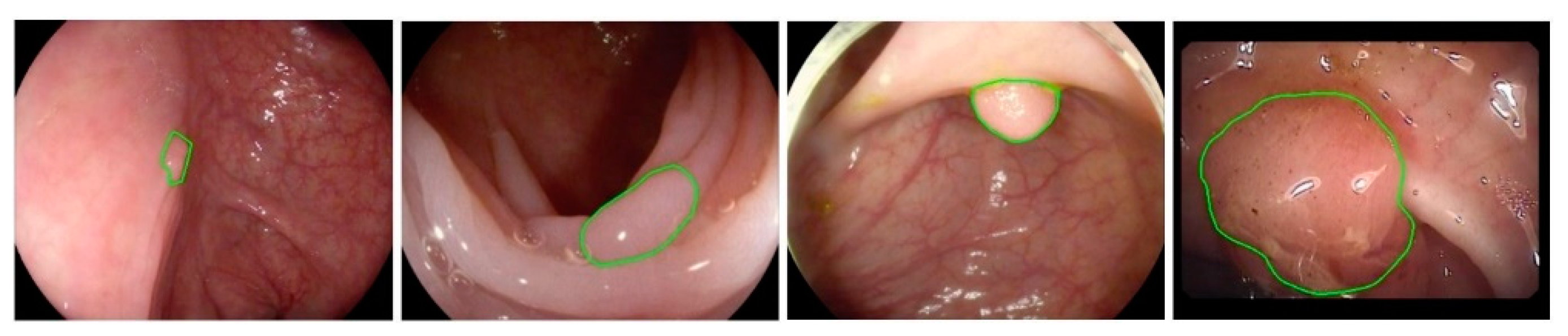
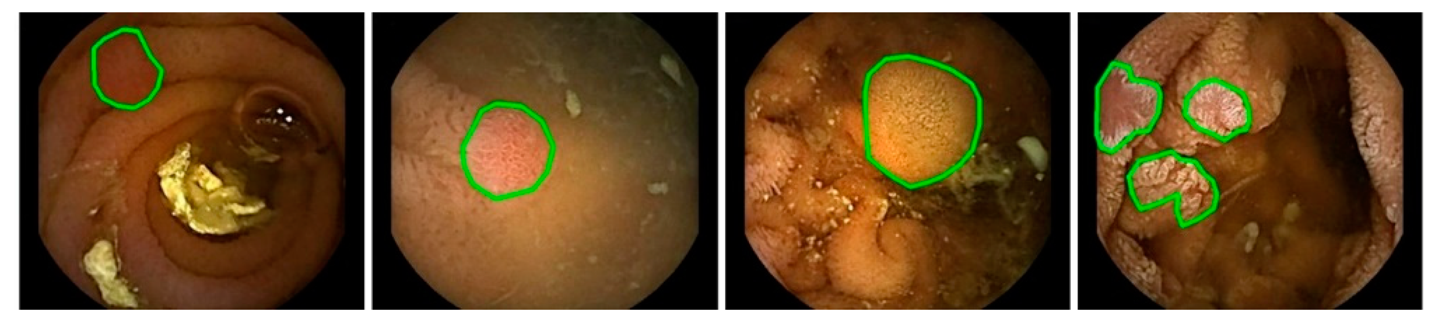
There are various challenges in the automated detection of polyps. As shown in Figure 1 and Figure 2, polyps appear in different sizes, shapes, textures, and color. Their endoscopic appearance can be similar to protruded lesions, flat elevated lesions, and flat lesions. The images even have noisy background with bleeding and endoluminal folds, which suppresses the accuracy of the detection process.
In the past few years, there have been many proposals made by various researchers to tackle the polyp detection challenge. A study with a common validation framework was provided as a part of the Medical Image Computing and Computer Assisted Intervention (MICCAI) sub-challenge on automatic polyp detection [21]. This has provided a consistent evaluation to assist polyp detection in colonoscopy images. The comparative analysis has proven that convolutional neural networks (CNN) were providing a state-of-the-art performance. Earlier approaches used feature extraction techniques. Color wavelet covariance (CWC) features along with linear discriminant analysis (LDA) [4] have been used to detect polyps in colonoscopy images. Textural features with support vector machine (SVM) were utilized for texture classification tasks [5]. Color and spatial features [6] and textural features [7] with SVM could outperform the approaches with textural features. Later, deep learning methods were employed to classify the polyp images in colonoscopy videos using CNN [10]. Small patches were extracted to increase the database, and CNN features were used to classify the polyp’s presence [11]. Hybrid methods were employed to boost the detection accuracy, such as a combination of edge detection and feature extraction to filter and refine polyp candidates with a voting scheme [12] to detect the polyps. Training a deep CNN is inappropriate with inadequate data. It has been shown [13] that in medical applications, even for polyp detection, fine-tuning a pre-trained model outperforms models trained from scratch. Another recent work [14], which adopted a Faster region-based convolutional neural network (R-CNN) approach [15] showed an improved performance in the detection of polyps by drawing bounding boxes around polyps and also employing post-learning schemes. Similarly, a VGG16-based Faster R-CNN model [16] was trained on 16 randomly selected sequences from colonoscopy videos. A SegNet-based CNN model [17] was employed to detect polyps using private data that contained 5545 colonoscopy images extracted from 1290 patients. The model was validated and tested on their internally collected colonoscopy image and video data. A news article [18] was also published based on the work from [17]. Various CNN models were trained on 8641 internally collected colonoscopy images, and the models were analyzed through sevenfold cross-validation [19]. A regression-based YOLO (you only look once) detection model was explored for polyp localization [20] on white light and narrow-band polyp images.
There are ongoing research studies with WCE videos to detect polyps. Geometric shape features along with textural features [22] were found to be helpful for polyp detection. An SVM-based polyp classification approach was applied with shape, color, and local texture feature extraction [23]. A frame-based binary classification of WCE videos was performed based on geometrical and texture content analysis [24]. Another SVM-based detection with statistical information from red–green–blue (RGB) channels was proposed to determine the polyp presence and extract the radii of the polyps [25]. Texture features integrated with wavelet transform, uniform local binary patterns, and SVM were studied [26]. Although deep learning has many approaches to analyzing natural images, very few works have been conducted on polyp detection in WCE images. A deep learning variant approach with a stacked sparse autoencoder with image manifold constraint [27] was explored to make the model learn and differentiate features from different classes to recognize frames containing polyps from WCE videos. Other methods concentrate on classifying different organs [28] and lesion detection [29] in WCE images. A survey paper [30,31] on video capsule endoscopy provides a better understanding of various models incorporating the detection and segmentation of polyps in the literature. However, all these methods performed polyp detection or the classification of frame-wise polyp presence.
This study mainly focuses on localization through segmentation and locating polyps in both colonoscopy and WCE still frames. The model evaluation is done by detecting the most probable polyp pixel points within the mask regions and locating the centroid representing the location of the polyp. An efficient deep learning approach is employed by applying a region-based convolutional neural network (R-CNN) along with data augmentation, feature extraction, and a fine-tuning model with pre-trained weights from well-established ImageNet [32] and Microsoft COCO (Common Objects in COntext) [33] datasets. Furthermore, the model is also fine-tuned with weights from flicker balloon data, which was fine-tuned from pre-trained COCO weights. This step is taken as an experiment to analyze the results that are obtained from the model, which is fine-tuned with polyp-like data in the natural images. The study confirms that the model performs better with improved localization on most of the polyp images compared to the other CNN approaches from the literature. The paper is the first of its kind to employ R-CNN to segment and locate polyp regions and analyze a model with various fine-tuned weights. The remainder of the paper is organized as follows. Section 2 provides details of the datasets utilized for the study and the methodology employed. In Section 3, we discuss the experiments conducted and present the results obtained. The conclusion for the study is presented in Section 4.
2. Materials and Methods
The datasets used for the study are augmented in the training phase, and the model is fine-tuned with pre-trained weights for detecting and segmenting polyps in both colonoscopy and WCE video frames. Figure 3 represents the overall flow of the model, which is discussed in detail in the following sections.
2.1. Datasets
The proposed approach is evaluated on two different datasets—still frames from colonoscopy and WCE—to solve the problem of polyp localization. The colonoscopy images are utilized from the MICCAI 2015 sub-challenge on automatic polyp detection [21] and GIANA (Gastrointestinal Image ANAlysis) 2018, which was part of Endoscopic Vision Challenge [34]. The WCE videos are provided by the Mayo Clinic.
The colonoscopy still frame analysis is performed using a publicly available polyp database from CVC-ClinicDB [35] for both training and tuning the proposed model and evaluating the CVC-ColonDB and CVC-PolypHD databases [35,36,37] and the ETIS-Larib [22] polyp database. The CVC-ClinicDB contains 612 standard definition still images of 384 × 288 resolution with 31 different polyps from 31 different sequences. The CVC-ColonDB database has 300 images of 500 × 574 resolution. The frames are extracted from 13 video sequences from 13 patients. The CVC-PolypHD contains 56 high-definition (1920 × 1080) images. Each of these still frame images has the presence of polyps along with an accurately segmented annotated ground truth mask. The ETIS-Larib is a polyp database that has 196 high-definition still images with a resolution of 1225 × 966 and 44 different polyps from 34 sequences. Table 1 gives a summary of all the colonoscopy databases used in the study.
The video database for wireless capsule endoscopy (WCE) is provided by the Mayo Clinic. The database has a total of 121 short videos from various patients. These are PillCam SB3 videos with 8:1 magnification and 30% higher resolution compared to SB2. PillCam SB3 and PillCam SB2 system allows direct visualization of small bowel. For the purposes of this study, a total of 1800 polyp-containing still frames were extracted from 18 different videos. Out of 1800 frames, 530 frames contained polyps. The ground truth segmentation masks were manually drawn and verified by expert clinicians. The proposed model was trained with 429 frames, and the rest were considered together as a validation dataset. The test dataset contained 55 frames decoded from WCE videos of various patients. There were a total of 67 polyps in 55 frames.
2.2. Data Augmentation
Deep learning models such as CNN require voluminous data to train the model without overfitting. This is the biggest challenge in the biomedical images [38]. The data that is available is limited, and most of them are raw images without annotations. This problem is overcome by applying data augmentation to the input images and the corresponding ground truths. In colonoscopy and WCE videos, polyps show variations in size, shape, color, and location. With these variations, it is best to generate duplicate data from the available image data by flipping, rotating, changing the scale, shearing, and blurring the images. These sets of augmentation are applied on 50% of each mini-batch of the input data before training. The remaining 50% data are left undisturbed.
Augmentation methods were chosen according to the appearance of the polyp images. Polyps change in shape and size, so image scaling and shear transform helped generate more data from the same image with different transformations. The images are rescaled from a range factor of 0.8 to 1.2 and shear transforms from a range between (−4,4). Polyps also appear to be in different locations; to encounter these locations, the images were flipped and rotated through a range between angles of (−180,180) degrees. Frames extracted from videos have the problem of motion blur, which lowers the quality of the image; to make the model generalize, Gaussian blur was applied on some of the images with a standard deviation varying from 0 to 1. Polyp images also have variations in brightening and darkening. To handle this problem, histogram equalization was applied on the images. We found from the experimental observations that histogram equalization degrades the performance of the model. This may be because the model finds it difficult to extract features from images that have enhanced contrast. These adjustments in the image intensities make the model differentiate the object pixels from the background. It is important to have a good quality image without losing the characteristics of the image while increasing the dataset through data augmentation.
2.3. Feature Extraction
The ResNet [39] models with depths of 50 layers or 101 layers act as feature extractors for the model to extract features over the entire image. These feature maps are further improved (to better represent the objects) by extracting more features from five different levels of ResNet layers. These levels are chosen so that the spatial dimension of the layer is reduced by half in the bottom–up view of the ResNet model. A top–down architecture with lateral connections is built to extract better feature maps at different scales. This network is called a Feature Pyramid Network (FPN) [40]. ResNet with FPN extracts features from different hierarchical levels with different scales so that each level has information of higher-level and lower-level features.
2.4. Region Proposals
The study recreates the Region Proposal Network (RPN) introduced in Faster R-CNN [15] to estimate the regions that are likely to scontain polyps within an image. Feature extraction and RPN together act as a first stage that scans an image and generate proposals. Proposals are small bounding box regions that are likely to contain an object (polyp). The RPN scans the features obtained from FPN in a convolution fashion with a small sliding window.
At each sliding window position, multiple region proposals (sets of boxes) were generated, which are called anchors; these have different sizes and different aspect ratios. Anchors help bind features to their raw location in the image. The RPN contains two separate fully connected layers to extract box probability scores (object or background) and bounding box deltas (box refinement). The targets of the RPN are ground-truth classes and ground-truth bounding boxes. Each anchor is assigned to a corresponding target by evaluating anchors based on intersection over union (IoU) values. The IoU values of the anchors are computed against the ground truth objects in the image. Positive anchors are the anchors whose IoU ≥0.7, anchors with IoU <0.7 and IoU ≥0.4 are considered neutral anchors, and anchors with IoU <0.4 are negative anchors, which do not cover any object. These values are empirically chosen. Neutral anchors are discarded and not used for training. Often, positive anchors do not cover objects completely, so the RPN performs regression with the bounding box deltas to shift and resize anchors according to the object location. Based on the RPN predictions, anchors are filtered according to their probability scores. The anchors that have a majority of their area overlapping with adjacent anchors are trimmed down to one anchor by choosing the one with the highest foreground score (non-maximum suppression). Finally, filtered proposals (RoI) are sent to the second stage.
2.5. Localization
The second stage forms network heads for generating binary masks. The region proposals from RPN are assigned to several specific regions of feature maps generated from FPN. These mapped regions are fed to the RoIAlign module [41], followed by convolutional layers and fully connected layers to predict the location and size of the predicted mask to fit the object. The RoIAlign module uses bilinear interpolation to properly align extracted features with the input image. Accurate mask segmentation is observed with the use of the RoIAlign module. This is implemented using TensorFlow’s crop and resize function. The mask generator network is built with the ROIAlign module followed by a stack of four convolutional layers with 3 × 3 receptive field filters and stride 1 with 256 channels. Later, a transposed convolution layer with 2 × 2 filter and stride 2 is included, and the final pixel-level probability mask output is generated from a 1 × 1 convolution layer with stride 1 and sigmoid activation function. All the convolution layers except for the final layer are built with the ReLU (rectified linear unit) activation function.
The resultant binary mask (28 × 28) corresponds to each region proposal, and the regions that have a class probability of 0.8 or higher are considered true predictions. During training, the ground truth masks for each instance are scaled down to 28 × 28 to compute the loss and backpropagate. During prediction, the predicted 28 × 28 binary masks are scaled up to the size of the corresponding region proposal bounding box. Based on the location information from the region proposals, all the successful mask predictions are stitched together to generate a final mask of the entire image. The output pixel-wise probability mask is further processed to locate the best pixel indicating the highest probability of being a polyp. If a region is identified as having the highest probability of being a polyp, then the centroid of the highly probable region is marked to the best location of the polyp from the mask.
We have used stochastic gradient descent (SGD) to optimize the loss function on each RoI region in the training phase as defined by L = Lmask [41].
2.6. Fine-Tuning
Fine-tuning is an efficient scheme in deep learning approaches that has been proven to have major improvements [13,42], especially when the CNN models are very deep, and the training data is sparse. The publicly available huge datasets of natural images provided by ImageNet [32] and Microsoft COCO [33] were used to train the deep CNN models. These weights were saved and utilized by loading them before training the model on the polyp dataset instead of random initialization of the weights. The ImageNet dataset is targeted for image classification tasks, which provides 1.28 M of train images and 50 K for validation with 1000 different categories. In contrast, the COCO dataset was developed by Microsoft to address the challenges of object detection, key point detection, caption generation, and object segmentation. Usually, the COCO dataset consists of 120 K training and validation images with the ability to categorize each instance among 80 categories.
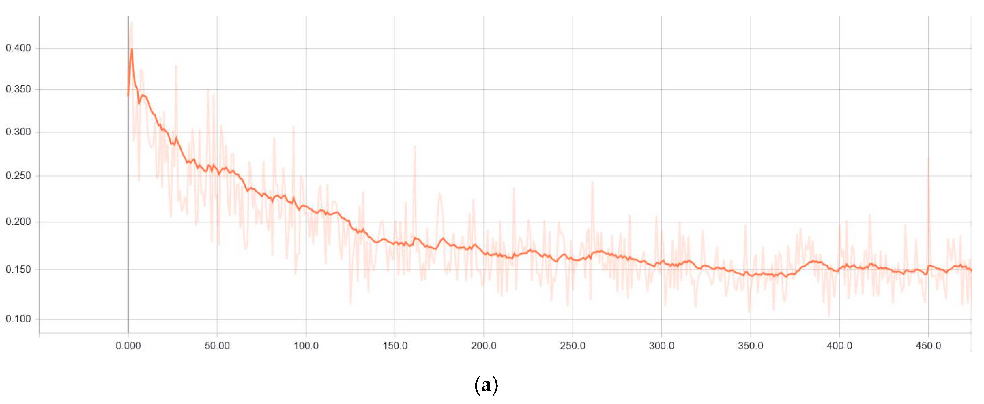
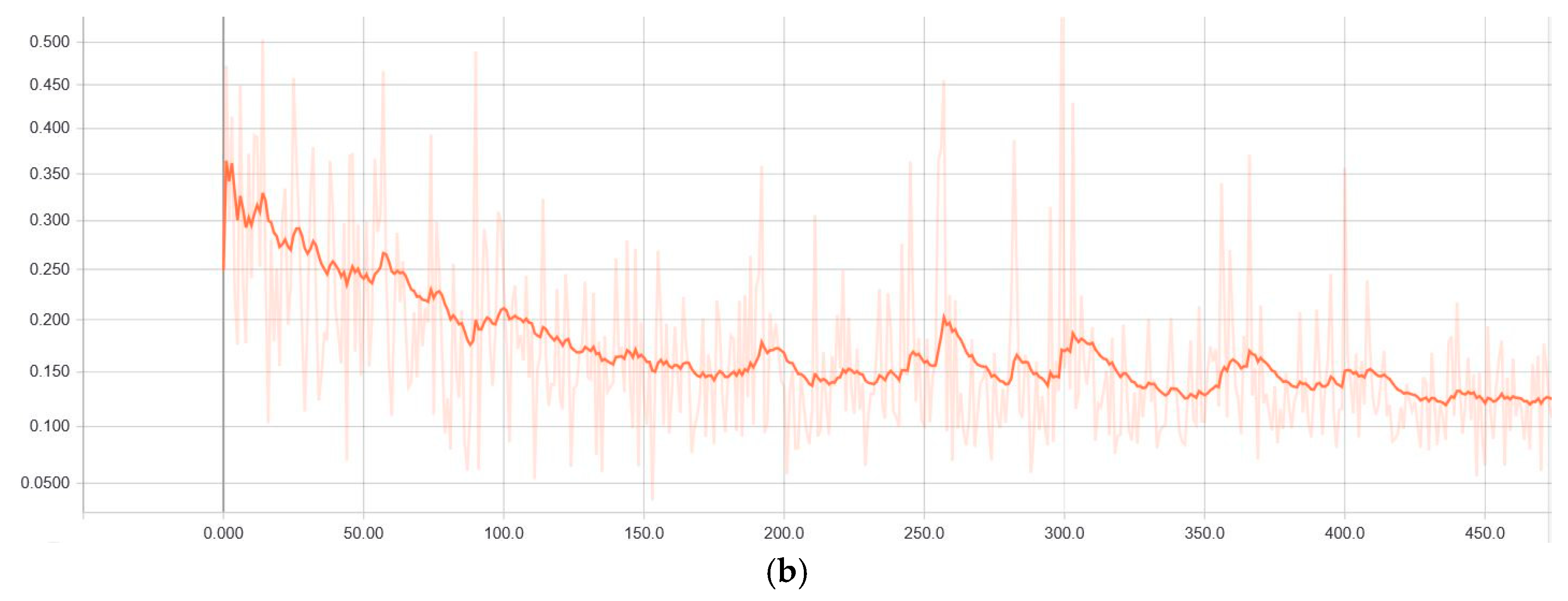
The ResNet model, which is used as a feature extractor model, is initially trained with both the ImageNet dataset and Microsoft COCO dataset. Additionally, 76 images of random balloon images from Flickr were annotated and considered as train and validation image data. These images were fine-tuned over pre-trained COCO weights. These three sets of weights were considered to fine-tune the ResNet model with polyp data. Each of these three sets of pre-trained weights were loaded into the ResNet model, and the weights were frozen while training the entire network (except the mask heads) with a relatively higher learning rate of 0.005 until it reached 100 epochs. Then, with a learning rate of 0.001, the entire model was trained without freezing any weights; that is, the weights of all the layers were updated for every epoch until there was an improvement in validation loss before reaching the 1000-epoch limit. These hyperparameters were empirically chosen. This strategy of updating only the mask head network during the initial epochs helps the randomly initialized mask head network weights adapt with the pre-trained ResNet backbone model, and the updates are made faster using a relatively higher learning rate. Later, the entire network weights were updated at a relatively lower learning rate to make sure that the whole network gradually learns the features from the polyp images. The training loss and validation loss curves are as shown in Figure 4. The curves indicate that the models are learning without overfitting, as the loss calculated from the unseen data (validation loss) follows the training loss curve. These curves are produced during the model training with ResNet-101 as the backbone with pre-trained weights from Flickr’s balloon data with early stopping. Early stopping avoids further training of the model when there is no improvement in validation loss detected in 20 consecutive epochs. This also helps avoid the problem of overfitting.
The complexity of the network is defined by its trainable parameters. The polyp localization model with ResNet-50 as the feature extractor has 44,603,678 trainable parameters, whereas the model with ResNet-101 as the feature extractor has 63,621,918 trainable parameters. The speed of the model is compared based on the average time taken by the model to predict a single image. The lower the time taken, the faster the model. It was found to be around 220.21 ms with the network with ResNet-50 as the feature extractor, and 317.01 ms with the network with ResNet-101 as the feature extractor. The computations are performed on an NVIDIA GeForce GTX 1080 8 GB GPU with a Nvidia CUDA Deep Neural Network (CuDNN) GPU-accelerated library installed.
3. Results and Discussion
This study implemented an R-CNN model using the Keras deep learning framework with a Tensorflow backend. The feature extractor part of the model extracted feature maps, and these features were scanned for region proposals with anchors at different levels with different scales of 8 × 8, 16 × 16, 32 × 32, 64 × 64, and 128 × 128 to make sure that the model could detect all the sizes of polyps with aspect ratios of 1:2, 2:1, and 1:1. The final region proposals contained positive and negative anchors. Each of these proposals were then processed to generate masks.
The masks were evaluated based on metrics as proposed by the MICCAI sub-challenge in order to make comparisons against other detection techniques. The location of the polyp marker in an image was considered as the baseline for polyp detection. A polyp marker that was inside the ground truth was considered as a true positive (TP). When there were multiple detections inside the same ground truth object, it was considered as one true positive. False positives (FP) were assigned to the detected polyp markers that fell outside the given ground truth. Every polyp misdetection was counted as a false negative (FN). There were no true negatives (TN), since there were no images with a complete absence of polyps. The metrics were calculated as follows:
where denotes precision, is recall, represents the F1 score, and represents the F2 score.
The detection points for TP, FP, and FN were marked based on the probability of each pixel in the final mask. A binary mask was created by thresholding the probability mask with the highest probability value within that mask. The centroid of the region formed was considered the detection point. The pixel-wise probability masks were analyzed and converted to heat maps to locate the best pixel position that represented the presence of the polyp in the image. This also helped to better understand the occurrence of false positives.
3.1. Colonoscopy Still Frame Analysis
Our model was trained with the CVC-ClinicDB database with 612 still frame polyp images. In the training phase, 536 images were used for training the model, and the remaining images were utilized as a validation dataset for tuning the model. The train dataset was split into mini-batches; each mini-batch had approximately 32 images. Data augmentation was randomly applied on 50% of the images in each mini-batch, and the remaining images were left undisturbed. The trained model weights were saved and loaded for predictions of testing datasets (the CVC-ColonDB, CVC-PolypHD, and ETIS-Larib datasets).
The ResNet model (ResNet-50 and ResNet-101) was trained individually with the CVC-ClinicDB polyp database and initialized with pre-trained weights from COCO, ImageNet, and Flickr’s balloon data. Table 2 illustrates the results from testing the model on the CVC-ColonDB database. The results from the CVC-PolypHD images are shown in Table 3. Table 4 gives the detection information from the ETIS-Larib database. There was no uniform performance from these datasets, as these data were extracted from different patients. On detailed observation, it could be found that the features extracted from ResNet-101 with Flickr’s balloon pre-trained weights tended to perform better with an optimal number of false positives and false negatives. This is understandable, because the ResNet-101 model has relatively deeper architecture that can extract more feature information from the image data, and the balloon data closely resembles the shape of the polyps. It was observed that there was no problem of overfitting with the deeper model, thanks to the image augmentation. This infers that the network is better at generalizing the polyp data. This can be observed from the learning curves (Figure 4) as well as from the prediction results on test datasets.
The still images from the ETIS-Larib database had a good comparison framework in the MICCAI sub-challenge. Table 5 compares the results from various submissions in the challenge, with the proposed approach having the best optimal results. The tabulated results are based on the predictions on the ETIS-Larib polyp database.
The top results are observed from the teams (CUMED, OUS, and UNS-UCLAN) that used a CNN-based fully convolutional network (FCN) for end-to-end learning. CUMED [43] employs multi-level feature representation with FCN for pixel-wise classification. OUS uses the AlexNet model [44] as the CNN with CaffeNet for the binary classification of the image patches to detect the presence of polyps. UNS-UCLAN trained three CNNs at three different scales for feature extraction and used a multi-layer perceptron (MLP) network for classification. It can be clearly seen that the proposed model outperforms the best model (CUMED) from the MICCAI sub-challenge. The proposed approach has more FP, which limited the precision value to 72.93. Most of these FP are due to the reflections of light on the mucosa and some polyp-like structures that are not actually polyps. FN are due to the misdetections of some challenging polyp shapes; there were very few of these in the training dataset. The proposed model competes with the CUMED model [43] and appears to outperform it in the polyp detection task.
Table 6 represents the evaluation results with and without data augmentation on the ETIS-Larib database. There is a huge performance improvement when the model is trained with differently oriented and transformed images. For every epoch, the model learns and tunes with a mixture of original data and augmented data. The results show a great margin of improvement by properly choosing the augmentation methodologies.
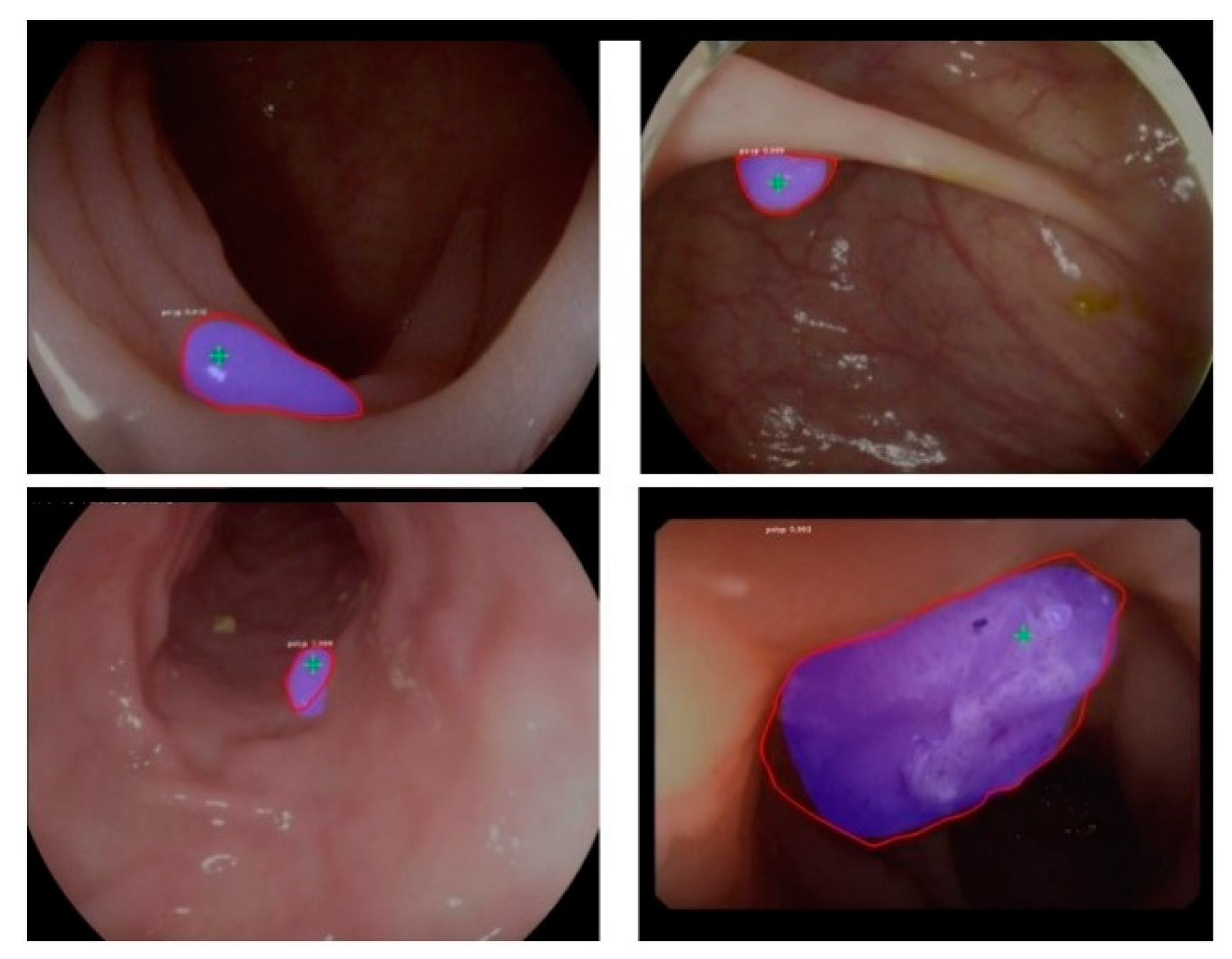
Figure 5 illustrates the ETIS-Larib polyp detection and segmentation results by the proposed model with the ResNet-101 model and pre-trained weights from Flickr’s balloon dataset.
3.2. WCE Video Analysis
A similar approach is employed for training and testing WCE videos for colonoscopy images, as mentioned earlier. Data augmentation is also applied on the training image dataset for the model to better generalize on different kinds of polyps. The results as shown in Figure 5 indicate the polyp detection and segmentation in the WCE videos. Table 7 illustrates the results from the WCE data. The tabulated values clearly indicate ResNet-101 as the best feature extractor, and the model trained on Flickr’s balloon pre-trained weights is clearly a winner.
There is no standard framework to compare the results with other techniques for the WCE polyp detection. It can be observed from the segmentation results that bubbles are detected as polyps; avoiding this misclassification is challenging due to limited frames with bubbles available to make the model learn that bubbles are not polyps. Some of the polyps look similar to the mucosa membrane, which makes it difficult for the model to segment on such polyps.
Table 8 provides an evaluation based on the segmentation results of the WCE polyp frames with and without data augmentation. Applying augmentation has helped the model learn more about the input data. A similar technique was employed for augmentation for colonoscopy images. The train dataset was split into mini-batches such that each mini-batch had 32 images and 50% of the randomly selected images in each mini-batch were augmented with different methods. The tabulated results show a higher detection of polyp images with data augmentation.
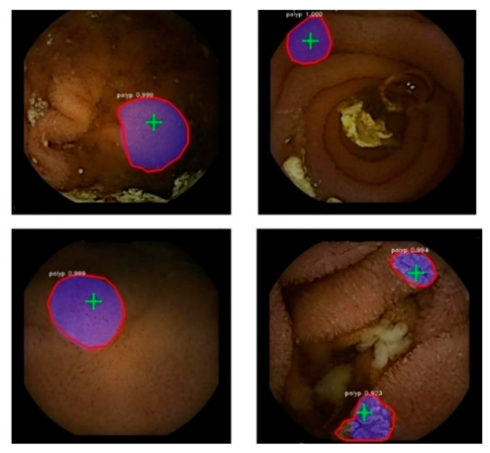
Figure 6 displays the detection and segmentation results on the WCE polyp test data based on the proposed approach with ResNet-101 and Flickr’s balloon data.
Although the model performs better in localizing polyps, there is still the possibility of improving the model. The first limitation for designing an automated polyp detection system is the limited availability of the data. Currently, additional data is generated online during training through data augmentation. Increasing the database with more polyp images will definitely improve the results and also help the model better generalize in its prediction of new polyp images. Recent studies on deep learning frameworks show improved classification and segmentation results on natural images with deeper architectures. However, there is a trade-off regarding the speed of training and testing the models. Deeper CNNs have a greater number of parameters that require more storage and GPU capability for better performance. In the future, the feature extractor part of the model can be replaced with deeper models to extract much better and more detailed feature maps. The second stage for generating a mask can be experimented with different combinations of architectures. The loss function plays a major role in backpropagation. If the loss function can be designed to better understand and differentiate the predicted output mask against the ground truth, there can be a gain in the performance. False positives and false negatives pose challenges in polyp detection performance. A detailed observation of the resultant images can result in better intuition and thus reduce false alarms. Lightening, bubbles, motion blur, etc. create the majority of false detections. Fine-tuning the model with false detection cases can be a good strategy to improve the performance of the model.
4. Conclusions
The study presents a deep learning-based automated polyp localization. The proposed approach is developed based on the region-based CNN. The feature maps generated using ResNet-101 and FPN have more details of a polyp image compared to ResNet-50 and FPN. This means that deeper models tend to extract more meaningful features from the images. The prediction score for each polyp is predicted based on the proposed regions from the feature maps. The model has successfully detected and accurately segmented the polyps in images. The added advantage of the proposed model compared to others is that it can produce an accurate segmentation for each polyp. The model shows better performance on the WCE video frames compared to colonoscopy images, and the results can be further improved if more annotated data is available.
Author Contributions
S.S. conducted research and testing of the proposed work while working at Xyken, LLC. F.M. assisted on testing and evaluation. S.Y. designed and supervised the research work.
Funding
This research work was supported by NIH Grant 5R43AG058269.
Acknowledgments
The WCE database was contributed and supported by Jonathan Leighton, Shabana Pasha, and Christine Gaudet, R.N. from Mayo Clinic.
Conflicts of Interest
The authors declare no conflict of interest.
References
- American Cancer Society. Cancer Facts & Figures 2019. Available online: https://www.cancer.org/research/cancer-facts-statistics/colorectal-cancer-facts-figures.html (accessed on 7 March 2019).
- Johnson, C.D.; Chen, M.; Toledano, A.Y.; Heiken, J.P.; Dachman, A.; Kuo, M.D.; Menias, C.O.; Siewert, B.; Cheema, J.I.; Obregon, R.G.; et al. Accuracy of CT Colonography for Detection of Large Adenomas and Cancers. N. Engl. J. Med. 2008, 359, 1207–1217. [Google Scholar] [CrossRef] [PubMed]
- Rabeneck, L.; El-Serag, H.B.; Davila, J.A.; Sandler, R.S. Outcomes of Colorectal Cancer in the United States: No Change in Survival (1986–1997). Am. J. Gastroenterol. 2018, 98, 471. [Google Scholar]
- Karkanis, S.A.; Iakovidis, D.K.; Maroulis, D.E.; Karras, D.A.; Tzivras, M. Computer-aided tumor detection in endoscopic video using color wavelet features. IEEE Trans. Inf. Technol. Biomed. 2003, 7, 141–152. [Google Scholar] [CrossRef] [PubMed] [Green Version]
- Iakovidis, D.K.; Maroulis, D.E.; Karkanis, S.A.; Brokos, A. A Comparative Study of Texture Features for the Discrimination of Gastric Polyps in Endoscopic Video. In Proceedings of the 18th IEEE Symposium on Computer-Based Medical Systems (CBMS’05), Dublin, Ireland, 23–24 June 2005; pp. 575–580. [Google Scholar] [CrossRef]
- Alexandre, L.A.; Nobre, N.; Casteleiro, J. Color and Position versus Texture Features for Endoscopic Polyp Detection. Int. Conf. Biomed. Eng. Inform. 2008, 2, 38–42. [Google Scholar]
- Cheng, D.-C.; Ting, W.-C.; Chen, Y.-F.; Jiang, X. Automatic Detection of Colorectal Polyps in Static Images. Biomed. Eng. Appl. Basis Commun. 2011, 23, 357–367. [Google Scholar] [CrossRef]
- Rajaraman, S.; Antani, S.K.; Poostchi, M.; Silamut, K.; Hossain, M.A.; Maude, R.J.; Jaeger, S.; Thoma, G.R. Pre-trained convolutional neural networks as feature extractors toward improved malaria parasite detection in thin blood smear images. PeerJ 2018, 6. [Google Scholar] [CrossRef]
- Sornapudi, S.; Stanley, R.J.; Stoecker, W.V.; Almubarak, H.; Long, R.; Antani, S.; Thoma, G.; Zuna, R.; Frazier, S.R. Deep Learning Nuclei Detection in Digitized Histology Images by Superpixels. J. Pathol. Inform. 2018, 9, 5. [Google Scholar] [CrossRef]
- Park, S.Y.; Sargent, D. Colonoscopic polyp detection using convolutional neural networks. In Proc. SPIE 9785, Medical Imaging 2016: Computer-Aided Diagnosis; International Society for Optics and Photonics: San Diego, CA, USA, 24 March 2016. [Google Scholar]
- Ribeiro, E.; Uhl, A.; Häfner, M. Colonic Polyp Classification with Convolutional Neural Networks. In Proceedings of the IEEE 29th International Symposium on Computer-Based Medical Systems (CBMS), Dublin, Ireland, 20–23 June 2016; pp. 253–258. [Google Scholar] [CrossRef]
- Tajbakhsh, N.; Gurudu, S.R.; Liang, J. Automated polyp detection in colonoscopy videos using shape and context information. IEEE Trans. Med. Imaging 2016, 35, 630–644. [Google Scholar] [CrossRef]
- Tajbakhsh, N.; Shin, J.Y.; Gurudu, S.R.; Hurst, R.T.; Kendall, C.B.; Gotway, M.B. Convolutional Neural Networks for Medical Image Analysis: Full Training or Fine Tuning? IEEE Trans. Med. Imaging 2016, 35, 1299–1312. [Google Scholar] [CrossRef]
- Shin, Y.; Qadir, H.A.; Aabakken, L.; Bergsland, J.; Balasingham, I. Automatic Colon Polyp Detection using Region based Deep CNN and Post Learning Approaches. IEEE Access 2018, 6, 40950–40962. [Google Scholar] [CrossRef]
- Ren, S.; He, K.; Girshick, R.; Sun, J. Faster R-CNN: Towards Real-time Object Detection with Region Proposal Networks. In Transactions on Pattern Analysis and Machine Intelligence, Proceedings of the 28th International Conference on Neural Information Processing Systems; MIT Press: Cambridge, MA, USA, 2015; Volume 1, pp. 91–99. [Google Scholar]
- Mo, X.; Tao, K.; Wang, Q.; Wang, G. An Efficient Approach for Polyps Detection in Endoscopic Videos Based on Faster R-CNN. In Proceedings of the 24th International Conference on Pattern Recognition (ICPR), Bejing, China, 20–24 August 2018; pp. 3929–3934. [Google Scholar] [CrossRef]
- Wang, P.; Xiao, X.; Brown, J.R.G.; Berzin, T.M.; Mengtian, T.; Xiong, F.; Hu, X.; Liu, P.; Song, Y.; Zhang, D.; et al. Development and validation of a deep-learning algorithm for the detection of polyps during colonoscopy. Nat. Biomed. Eng. 2018, 2, 741–748. [Google Scholar] [CrossRef] [PubMed]
- Mori, Y.; Kudo, S. Detecting colorectal polyps via machine learning. Nat. Biomed. Eng. 2018, 713–714. [Google Scholar] [CrossRef] [PubMed]
- Urban, G.; Tripathi, P.; Alkayali, T.; Mittal, M.; Jalali, F.; Karnes, W.; Baldi, P. Deep Learning Localizes and Identifies Polyps in Real Time With 96% Accuracy in Screening Colonoscopy. Gastroenterology 2018, 155, 1069–1078. [Google Scholar] [CrossRef] [PubMed]
- Zheng, Y.; Zhang, R.; Yu, R.; Jiang, Y.; Mak, T.W.C.; Wong, S.H.; Lau, J.Y.W.; Poon, C.C.Y. Localisation of Colorectal Polyps by Convolutional Neural Network Features Learnt from White Light and Narrow Band Endoscopic Images of Multiple Databases. In Proceedings of the 40th Annual International Conference of the IEEE Engineering in Medicine and Biology Society (EMBC), Honolulu, HI, USA, 17–21 July 2018; pp. 4142–4145. [Google Scholar]
- Bernal, J.; Tajkbaksh, N.; Sanchez, F.J.; Matuszewski, B.J.; Hao, C.; Lequan, Y.; Angermann, Q.; Romain, O.; Rustad, B.; Balasingham, I.; et al. Comparative Validation of Polyp Detection Methods in Video Colonoscopy: Results from the MICCAI 2015 Endoscopic Vision Challenge. IEEE Trans. Med. Imaging 2017, 36, 1231–1249. [Google Scholar] [CrossRef]
- Silva, J.; Histace, A.; Romain, O.; Dray, X.; Granado, B. Toward embedded detection of polyps in WCE images for early diagnosis of colorectal cancer. Int. J. Comput. Assist. Radiol. Surg. 2014, 9, 283–293. [Google Scholar] [CrossRef]
- Figueiredo, I.; Kumar, S.; Figueiredo, P. An Intelligent System for Polyp Detection in Wireless Capsule Endoscopy Images. In Proceedings of the IV ECCOMAS Thematic Conference on Computational Vision and Medical Image Processing, Madeira Island, Funchal, Portugal, 14–16 October 2013. [Google Scholar] [CrossRef]
- Mamonov, A.V.; Figueiredo, I.N.; Figueiredo, P.N.; Tsai, Y.R. Automated Polyp Detection in Colon Capsule Endoscopy. IEEE Trans. Med. Imaging 2014, 33, 1488–1502. [Google Scholar] [CrossRef]
- Zhou, M.; Bao, G.; Geng, Y.; Alkandari, B.; Li, X. Polyp Detection and Radius Measurement in Small Intestine Using Video Capsule Endoscopy. In Proceedings of the 7th International Conference on Biomedical Engineering and Informatics, Dalian, China, 14–16 October 2014; pp. 237–241. [Google Scholar] [CrossRef]
- Li, B.; Meng, M.Q.H. Automatic polyp detection for wireless capsule endoscopy images. Expert Syst. Appl. 2012, 39, 10952–10958. [Google Scholar] [CrossRef]
- Yuan, Y.; Meng, M.Q.H. Deep learning for polyp recognition in wireless capsule endoscopy images. Med. Phys. 2017, 44, 1379–1389. [Google Scholar] [CrossRef] [Green Version]
- Yu, J.; Chen, J.; Xiang, Z.Q.; Zou, Y. A Hybrid Convolutional Neural Networks with Extreme Learning Machine for WCE Image Classification. In Proceedings of the IEEE International Conference on Robotics and Biomimetics (ROBIO), Zhuhai, China, 6–9 December 2015; pp. 1822–1827. [Google Scholar] [CrossRef]
- Zhu, R.; Zhang, R.; Xue, D. Lesion Detection of Endoscopy Images Based on Convolutional Neural Network Features. In Proceedings of the 8th International Congress on Image and Signal. Processing (CISP), Shenyang, China, 14–16 October 2015; pp. 372–376. [Google Scholar] [CrossRef]
- Prasath, V.B.S. Polyp Detection and Segmentation from Video Capsule Endoscopy: A Review. J. Imaging 2016, 3, 1. [Google Scholar] [CrossRef]
- Alagappan, M.; Brown, J.R.G.; Mori, Y.; Berzin, T.M. Artificial intelligence in gastrointestinal endoscopy: The future is almost here. World J. Gastrointest. Endosc. 2018, 10, 239–249. [Google Scholar] [CrossRef] [PubMed]
- Deng, J.; Dong, W.; Socher, R.; Li, L.; Li, K.; Li., F.F. ImageNet: A Large-Scale Hierarchical Image Database. In Proceedings of the IEEE Conference on Computer Vision and Pattern Recognition (CVPR’09), Miami Beach, FL, USA, 20–25 June 2009. [Google Scholar]
- Lin, T.Y.; Maire, M.; Belongie, S.; Hays, J.; Perona, P.; Ramanan, D.; Dollar, P.; Zitnick, C.L. Microsoft COCO: Common Objects in Context. In Computer Vision ECCV 2014; Fleet, D., Pajdla, T., Schiele, B., Tuytelaars, T., Eds.; Springer International Publishing: New York, NY, USA, 2014; pp. 740–755. [Google Scholar] [Green Version]
- Endoscopic Vision Challenge. Sub-challenge: Gastrointestinal Image ANAlysis (GIANA). Available online: https://giana.grand-challenge.org (accessed on 21 June 2018).
- Bernal, J.; Sánchez, F.J.; Fernández-Esparrach, G.; Gil, D.; Rodríguez, C.; Vilariño, F. WM-DOVA maps for accurate polyp highlighting in colonoscopy: Validation vs. saliency maps from physicians. Comput. Med. Imaging Graph. 2015, 43, 99–111. [Google Scholar] [CrossRef] [PubMed]
- Vázquez, D.; Vázquez, D.; Bernal, J.; Sánchez, F.J.; Fernández-Esparrach, G.; López, A.M.; Romero, A.; Drozdzal, M.; Courville, A. A Benchmark for Endoluminal Scene Segmentation of Colonoscopy Images. J. Healthcare Eng. 2017, 2017, 9. [Google Scholar] [CrossRef]
- Bernal, J.; Sánchez, F.J.; Vilariño, F. Towards automatic polyp detection with a polyp appearance model. Pattern Recognit. 2012, 45, 3166–3182. [Google Scholar] [CrossRef]
- Kohli, M.D.; Summers, R.M.; Geis, J.R. Medical Image Data and Datasets in the Era of Machine Learning—Whitepaper from the 2016 C-MIMI Meeting Dataset Session. J. Digit. Imaging 2017, 30, 392–399. [Google Scholar] [CrossRef] [PubMed]
- He, K.; Zhang, X.; Ren, S.; Sun, J. Deep residual learning for image recognition. Proc. IEEE 2016, 770–778. [Google Scholar]
- Lin, T.Y.; Dollar, P.; Girshick, R.; He, K.; Hariharan, B.; Belongie, S. Feature Pyramid Networks for Object Detection. In Proceedings of the 30th IEEE Conference Computer Vision Pattern Recognition, CVPR, Honolulu, HI, USA, 21–26 July 2017; pp. 936–944. [Google Scholar]
- He, K.; Gkioxari, G.; Dollár, P.; Girshick, R. Mask R-CNN. In Proceedings of the IEEE International Conference on Computer Vision (ICCV), Venice, Italy, 22–29 October 2017; pp. 2980–2988. [Google Scholar] [CrossRef]
- Bae, S.; Yoon, K. Polyp Detection via Imbalanced Learning and Discriminative Feature Learning. IEEE Trans. Med. Imaging 2005, 34, 2379–2393. [Google Scholar] [CrossRef]
- Chen, H.; Qi, X.; Cheng, J.; Heng, P. Deep Contextual Networks for Neuronal Structure Segmentation. In Proceedings of the 30th Conference on Artificial Intelligence (AAAI 2016), Phoenix, AZ, USA, 12–17 February 2016; pp. 1167–1173. [Google Scholar]
- Krizhevsky, A.; Sutskever, I.; Hinton, G. ImageNet Classification with Deep Convolutional Neural Networks. Adv. Neural Inf. Process. Syst. (Nips) 2012, 25, 1097–1105. [Google Scholar] [CrossRef]
Figure 1.
Images with ground truth polyps (marked in green) from colonoscopy videos.

Figure 2.
Images with ground truth polyps (marked in green) from wireless capsule endoscopy (WCE) videos.
Figure 2.
Images with ground truth polyps (marked in green) from wireless capsule endoscopy (WCE) videos.

Figure 3.
Flowchart depicting the proposed approach.

Figure 4.
Loss curves (loss vs. epochs) during the (a) training phase and (b) validation phase.


Figure 5.
Polyp segmentation in colonoscopy images (ETIS-Larib). Blue overlay is the predicted segmentation mask. The contour of the ground truth masks is shown in red. Detection points are masked in green.
Figure 5.
Polyp segmentation in colonoscopy images (ETIS-Larib). Blue overlay is the predicted segmentation mask. The contour of the ground truth masks is shown in red. Detection points are masked in green.

Figure 6.
Polyp segmentation in WCE video frames. Blue overlay indicates the predicted segmentation mask. The contour of the ground truth masks is shown in red. Detection points are masked in green.
Figure 6.
Polyp segmentation in WCE video frames. Blue overlay indicates the predicted segmentation mask. The contour of the ground truth masks is shown in red. Detection points are masked in green.


Table 1.
Summary of colonoscopy databases.
| Database | Purpose | Resolution | # Patients | # Sequences | # Images |
|---|---|---|---|---|---|
| CVC-ClinicDB | Training | 384 × 288 | 23 | 31 | 612 SD frames |
| CVC-ColonDB | Testing | 500 × 574 | 13 | 13 | 300 SD frames |
| CVC-PolypHD | Testing | 1920 × 1080 | - | - | 56 HD frames |
| ETIS-Larib | Testing | 1225 × 966 | - | 34 | 196 HD frames |
Table 2.
Results from testing on CVC-ColonDB polyp data. COCO: Common Objects in Context, TP: true positives, FP: false positives, FN: false negatives.
Table 2.
Results from testing on CVC-ColonDB polyp data. COCO: Common Objects in Context, TP: true positives, FP: false positives, FN: false negatives.
| Model Backbone | Pre-Trained Weights | TP | FP | FN | P | R | F1 | F2 |
|---|---|---|---|---|---|---|---|---|
| Resnet-101 | COCO | 271 | 39 | 28 | 87.42 | 90.64 | 89.00 | 89.97 |
| ImageNet | 280 | 45 | 19 | 86.15 | 93.65 | 89.74 | 92.04 | |
| Balloon | 274 | 31 | 25 | 89.94 | 91.64 | 90.73 | 91.27 | |
| Resnet-50 | COCO | 274 | 95 | 25 | 74.25 | 91.64 | 82.04 | 87.54 |
| ImageNet | 287 | 77 | 12 | 78.85 | 96.00 | 86.58 | 92.00 | |
| Balloon | 276 | 104 | 23 | 72.63 | 92.31 | 81.30 | 87.56 |
Table 3.
Results from testing on CVC-PolypHD polyp data.
| Model Backbone | Pre-Trained Weights | TP | FP | FN | P | R | F1 | F2 |
|---|---|---|---|---|---|---|---|---|
| Resnet-101 | COCO | 47 | 8 | 17 | 85.45 | 73.44 | 79.00 | 75.56 |
| ImageNet | 49 | 8 | 15 | 85.96 | 76.56 | 81.00 | 78.27 | |
| Balloon | 50 | 10 | 14 | 83.33 | 78.12 | 80.65 | 79.11 | |
| Resnet-50 | COCO | 52 | 12 | 12 | 81.25 | 81.25 | 81.25 | 81.25 |
| ImageNet | 50 | 9 | 14 | 84.75 | 78.12 | 81.30 | 79.37 | |
| Balloon | 48 | 8 | 16 | 85.71 | 75.00 | 80.00 | 76.92 |
Table 4.
Results from testing on ETIS-Larib polyp data.
| Model Backbone | Pre-Trained Weights | TP | FP | FN | P | R | F1 | F2 |
|---|---|---|---|---|---|---|---|---|
| Resnet-101 | COCO | 161 | 58 | 47 | 73.52 | 77.40 | 75.41 | 76.59 |
| ImageNet | 160 | 63 | 48 | 71.75 | 76.92 | 74.25 | 75.83 | |
| Balloon | 167 | 62 | 41 | 72.93 | 80.29 | 76.43 | 78.70 | |
| Resnet-50 | COCO | 146 | 116 | 62 | 55.73 | 70.19 | 62.13 | 66.73 |
| ImageNet | 160 | 93 | 48 | 63.24 | 76.92 | 69.41 | 73.73 | |
| Balloon | 141 | 86 | 67 | 62.11 | 67.79 | 64.83 | 66.57 |
Table 5.
Comparison of proposed approach with various state-of-the-art polyp localization methods on the ETIS-Larib database.
Table 5.
Comparison of proposed approach with various state-of-the-art polyp localization methods on the ETIS-Larib database.
| TP | FP | FN | P | R | F1 | F2 | |
|---|---|---|---|---|---|---|---|
| Proposed approach 1 | 167 | 62 | 41 | 72.93 | 80.29 | 76.43 | 78.70 |
| CUMED | 144 | 55 | 64 | 72.3 | 69.2 | 70.7 | 69.8 |
| OUS | 131 | 57 | 77 | 69.7 | 63.0 | 66.1 | 64.2 |
| UNS-UCLAN | 110 | 226 | 98 | 32.73 | 52.8 | 40.4 | 47.1 |
| PLS | 119 | 630 | 89 | 15.8 | 57.2 | 24.9 | 37.6 |
| ETIS-LARIB | 103 | 1373 | 105 | 6.9 | 49.5 | 12.2 | 22.3 |
| SNU | 20 | 176 | 188 | 10.2 | 9.6 | 9.9 | 9.7 |
1 Model trained with ResNet-101 as the backbone with pre-trained weights from Flickr’s balloon data.
Table 6.
Results with and without data augmentation on ETIS-Larib polyp data.
| TP | FP | FN | P | R | F1 | F2 | |
|---|---|---|---|---|---|---|---|
| W/o data augmentation 1 | 147 | 73 | 61 | 66.82 | 70.67 | 68.69 | 69.87 |
| With data augmentation 1 | 167 | 62 | 41 | 72.93 | 80.29 | 76.43 | 78.70 |
1 Model trained with ResNet-101 as the backbone with pre-trained weights from Flickr’s balloon data.
Table 7.
Results from testing on the Mayo Clinic wireless capsule endoscopy (WCE) polyp data.
| Model Backbone | Pre-Trained Weights | TP | FP | FN | P | R | F1 | F2 |
|---|---|---|---|---|---|---|---|---|
| Resnet-101 | COCO | 63 | 4 | 4 | 94.03 | 94.03 | 94.03 | 94.03 |
| ImageNet | 64 | 14 | 3 | 82.05 | 95.52 | 88.28 | 92.49 | |
| Balloon | 64 | 1 | 3 | 98.46 | 95.52 | 96.67 | 96.10 | |
| Resnet-50 | COCO | 64 | 4 | 3 | 94.12 | 95.52 | 94.81 | 95.24 |
| ImageNet | 58 | 5 | 9 | 92.06 | 86.57 | 89.23 | 87.61 | |
| Balloon | 63 | 7 | 4 | 90.00 | 94.03 | 91.97 | 93.20 |
Table 8.
Results with and without data augmentation on Mayo Clinic WCE polyp data.
| TP | FP | FN | P | R | F1 | F2 | |
|---|---|---|---|---|---|---|---|
| w/o data augmentation 1 | 50 | 4 | 17 | 92.59 | 74.63 | 82.64 | 77.64 |
| With data augmentation 1 | 64 | 1 | 3 | 98.46 | 95.52 | 96.67 | 96.10 |
1 Model trained with ResNet-101 as the backbone with pre-trained weights from Flickr’s balloon data.
© 2019 by the authors. Licensee MDPI, Basel, Switzerland. This article is an open access article distributed under the terms and conditions of the Creative Commons Attribution (CC BY) license (http://creativecommons.org/licenses/by/4.0/).
Share and Cite
MDPI and ACS Style
Sornapudi, S.; Meng, F.; Yi, S. Region-Based Automated Localization of Colonoscopy and Wireless Capsule Endoscopy Polyps. Appl. Sci. 2019, 9, 2404. https://doi.org/10.3390/app9122404
AMA Style
Sornapudi S, Meng F, Yi S. Region-Based Automated Localization of Colonoscopy and Wireless Capsule Endoscopy Polyps. Applied Sciences. 2019; 9(12):2404. https://doi.org/10.3390/app9122404
Chicago/Turabian StyleSornapudi, Sudhir, Frank Meng, and Steven Yi. 2019. "Region-Based Automated Localization of Colonoscopy and Wireless Capsule Endoscopy Polyps" Applied Sciences 9, no. 12: 2404. https://doi.org/10.3390/app9122404
Note that from the first issue of 2016, this journal uses article numbers instead of page numbers. See further details here.