Sound Source Localization Fusion Algorithm and Performance Analysis of a Three-Plane Five-Element Microphone Array

Abstract

To reduce the negative effect on sound source localization when the source is at an extreme angle and improve localization precision and stability, a theoretical model of a three-plane five-element microphone array is established, using time-delay values to judge the sound source’s quadrant position. Corresponding judgment criteria were proposed, solving the problem in which a single-plane array easily blurs the measured position. Based on sound source geometric localization, a formula for the sound source azimuth calculation of a single-plane five-element microphone array was derived. The sinusoids and cosines of two elevation angles based on two single-plane arrays were introduced into the sound source spherical coordinates as composite weighted coefficients, and a sound source localization fusion algorithm based on a three-plane five-element microphone array was proposed. The relationship between the time-delay estimation error, elevation angle, horizontal angle, and microphone array localization performance was discussed, and the precision and stability of ranging and direction finding were analyzed. The results show that the measurement precision of the distance from the sound source to the array center and the horizontal angle are improved one to threefold, and the measurement precision of the elevation angle is improved one to twofold. Although there is a small error, the overall performance of the sound source localization is stable, reflecting the advantages of the fusion algorithm.

1. Introduction

A signal represents the physical quantity of a message. Humans can collect important information about the environment through a signal, especially a sound source signal [1,2,3,4,5], which is a sound wave generated by the vibration of an object, as well as the movement of a sound wave through any material. As a kind of wave, sound with a frequency between 20 Hz and 20 kHz can be recognized by the human ear [6,7]. Moreover, a target sound source can be located by receiving the sound source signal and applying an algorithm. Microphone arrays [8,9,10,11] perform functions such as noise elimination and target tracking. They can also be used to passively receive sound source signals, making it practical for researchers to collect signals. A microphone array system is composed of multiple microphones placed in accordance with a given topological structure that performs real-time processing on spatial sound source signals received from different directions. In recent years, with the rapid development of physics [12], mathematics [13], and signal processing [14], sound source localization technology for microphone arrays has received widespread attention from researchers both domestically and abroad. In addition, research on sound detection technology for the design of microphone arrays and sound source localization algorithms [15,16,17,18,19] has been conducted.

In terms of sound source localization technology, foreign countries have had an earlier start. In 1985, Flanagan [20] used a linear array as a research tool to determine the available bandwidth as a function of the steering direction, given the number and spacing of receiving microphones, and solved the problem of reducing the available bandwidth of space discrimination when turning away from the normal wave arrival direction. In 1997, Brandstein et al. [21] used a set of microphones designed to provide a high-quality source localization while attenuating the interference of speech and ambient noise without the need for a local position sensor, an obstructive talking handheld, or a microphone, as a single microphone does not have this function. In 2016, Miao F et al. [22] extended traditional triangulation to moving sources. The experiment proved that the moving time difference of arrival (MTDOA) method is superior to traditional triangulation in case of moving sound sources.

With the rapid development of modern technology, numerous breakthroughs in sound source detection have been made. In 2010, XJ Liu et al. [23] proposed a moving sound source tracking method based on microphone array measurements that uses the speech linear prediction residual to estimate the time delay, therefore weakening the noise and reverberation effect and significantly improving localization precision. In 2013, Qinqi Xu et al. [24], using an acoustic array in a robotic system, proposed a tetrahedral array to locate a sound source target. Using the time difference localization method, the paper deduced localization and fallibility formulas. The method not only improves the localization precision, but also reduces the blind space. In 2017, Alon et al. [25] proposed a method to overcome the effect of spatial aliasing via signal processing. A 32-element spherical microphone array was used to extend the frequency range of the microphone array, and experiments verified the precision of the theoretical results to overcome the aliasing. In the same year, Su et al. [26] proposed a linear microphone array with multiple hypothesis tracking, combined with a novel sound source parameterization, the joint optimization of six sensors, and three landmarks and sound source positions to solve the three-dimensional sound source mapping problem. Due to the unremitting exploration of international researchers, studies on sound source localization technology based on multi-microphone arrays have been rapidly developing.

The estimated arrival time delay will cause errors [27,28,29], and the errors of ranging and direction-finding are difficult to avoid. When the elevation angle is near the extreme angles of either zero or 90°, the error will be more obvious, which clearly affects the precision and stability of the sound source localization.

The problem is that the precision and stability of the sound source are adversely impacted by the sound source at an extreme angle. Therefore, in this paper, based on the analysis of a sound source geometry localization algorithm, a theoretical model for a five-element microphone array is established, using the time-delay values to determine the quadrant of the sound source position to solve the problem in which a single-plane array is prone to producing azimuth blurring. By deducing the formula of the sound source position calculation in a single-plane array, the sine and cosine values of the two elevation angles are used as weighting coefficients and are introduced into the sound source spherical coordinate formula. A sound source localization fusion algorithm of a three-plane five-element microphone array is proposed for studying sound source localization. According to the error analysis formula, the relationship between the ranging and direction-finding precision and the array element spacing, horizontal angle, elevation angle, and time-delay estimation error are obtained, and the performance of the sound source localization is analyzed. By experimentally adjusting the sound source position and array element spacing, the fusion algorithm is used to obtain the sound source coordinates. Based on forward data, the measured data are compared and analyzed.

In this paper, the proposed sound source localization fusion algorithm was used to locate the actual sound source, and compare it with theoretical data, radar chart data, and important literature. The experimental results showed that by appropriately increasing the array element spacing of the three-plane five-element microphone array, the sound source position could be measured more accurately and stably than the single-plane array. At the same time, the thunder source point data measured by the fusion algorithm could be used to provide data feedback for thunderstorm cloud forecast warnings, and could be used to track the moving path of the thunderstorm cloud in real time. In particular, the fusion algorithm could effectively reduce the negative impact of the sound source at an extreme angle on localization performance, and these conclusions were not achievable with existing sound source localization algorithms.

In Section 2, we analyzed the finite element microphone array theory, established a three-plane five-element microphone array model, and gave the quadrant judgment criteria for the location of the sound source. In Section 3, aiming at the problem that the sound source at an extreme angle had a negative impact on the performance of sound source localization, we proposed a sound source localization fusion algorithm and gave its calculation steps. In Section 4, based on the theory of indirect measurement error, we analyzed the error generated by the fusion algorithm for sound source localization, and theoretically supported the effectiveness of the algorithm. In Section 5, indoor, outdoor, and contrast experiments were performed using the fusion algorithm, and performance comparisons were compared with the latest relevant literature. In the last part, the application prospect of the sound source localization fusion algorithm was prospected, and the consideration of the next research work was given.

2. Three-Plane Five-Element Microphone Array Model

The cost of the algorithm research and the complexity of data processing should be considered when selecting the number of microphones. If too few microphones are selected, the microphone array [8,9,10,11] will not receive enough information, which greatly affects the precision analysis of the localization algorithm, whereas too many microphones will increase the cost and complexity.

2.1. Establishment of a Three-Plane Five-Element Microphone Array Model

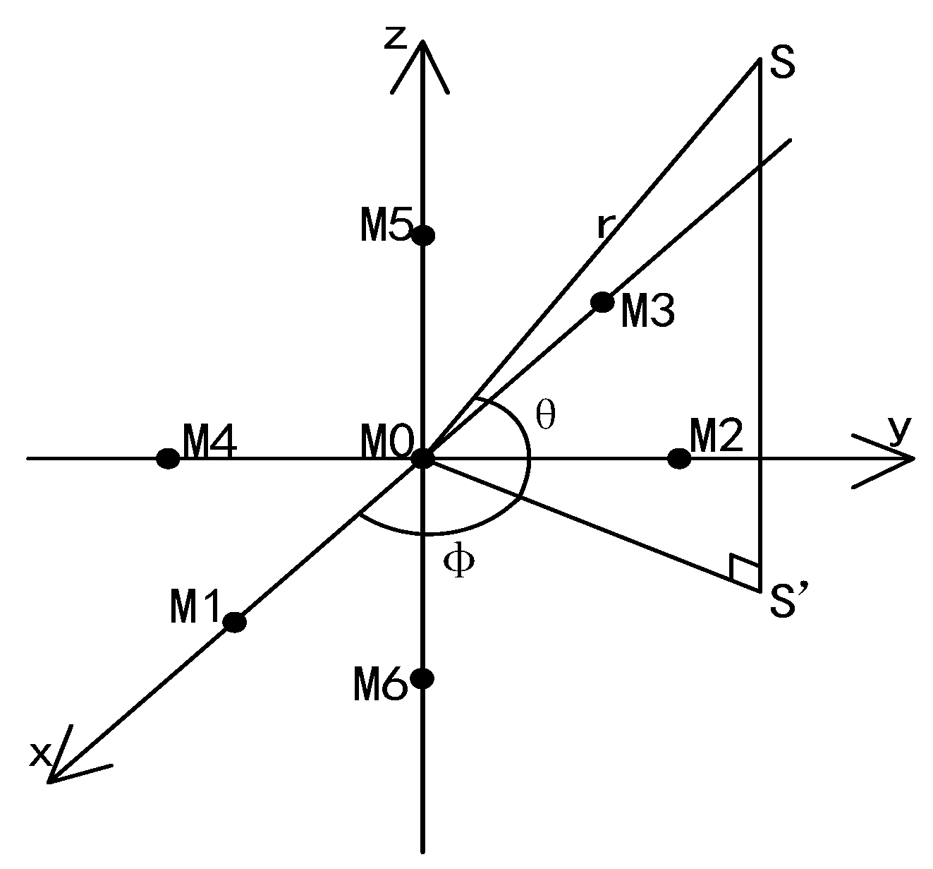
The model of the established three-plane five-element microphone array is shown in Figure 1.

The array consists of seven microphones: M0, M1, M2, M3, M4, M5, and M6. The first single-plane five-element microphone array is composed of four microphones in the X0Y plane—M1, M2, M3, and M4—and M0. The second single-plane five-element microphone array is composed of four microphones in the X0Z plane—M1, M3, M5, and M6—and M0. The third single-plane five-element microphone array is composed of four microphones in the Y0Z plane—M2, M4, M5, and M6—and M0. All three five-element microphone arrays use M0 as the reference microphone. The microphone M0 is located at the origin (0,0,0). It is assumed that the distances between the remaining six microphones and the origin of the coordinates are all a; then, the coordinates of each microphone can be expressed as M1 (a, 0, 0), M2 (0, a, 0), M3 (−a, 0, 0), M4 (0, −a, 0), M5 (0, 0, a), and M6 (0, 0, −a). It is defined that the time that it takes for S to propagate to microphones M0, M1, M2, M3, M4, M5, and M6 is t₀, $t_1$, $t_2$, $t_3$, $t_4$, $t_5$, and $t_6$, respectively. Based on the model, the relative time-delay values of six groups are set as ${\tau }_{10}=t_1-t_0$, ${\tau }_{20}=t_2-t_0$, ${\tau }_{30}=t_3-t_0$, ${\tau }_{40}=t_4-t_0$, ${\tau }_{50}=t_5-t_0$, and ${\tau }_{60}=t_6-t_0$. The coordinates of the sound source S are S (x, y, z) in the Cartesian coordinate system and S($r$,$\theta$,$\phi$) in the spherical coordinate system. The distance between the sound source S and M0 is $r$, the projection point of S on the X0Y plane is S′, the elevation angle S0S′ is $\theta$, and the horizontal angle X0S′ is $\phi$. The target sound source S generates sound waves propagating in the form of spherical waves with a propagation speed of c.

2.2. Judgment Criteria for the Sound Source Position Quadrant

Using the microphone M0 as the reference microphone, the times for the target sound source to transmit to the seven microphones are not the same, and six sets of mutually independent time-delay values can be obtained: ${\tau }_{10}$, ${\tau }_{20}$, ${\tau }_{30}$, ${\tau }_{40}$, ${\tau }_{50}$, and ${\tau }_{60}$, which are also all different. Based on the size relationship between the six groups of the time-delay value, the judgment criteria of the quadrant of the sound source position in the coordinate system are given in

Table 1. Criteria for judging the sound source position quadrant.

Basis of Judgment	Quadrant
${\tau }_{30}$ > ${\tau }_{10}$; ${\tau }_{40}$ > ${\tau }_{20}$; ${\tau }_{60}$ > ${\tau }_{50}$	first quadrant
${\tau }_{30}$ < ${\tau }_{10}$; ${\tau }_{40}$ > ${\tau }_{20}$; ${\tau }_{60}$ > ${\tau }_{50}$	second quadrant
${\tau }_{30}$ < ${\tau }_{10}$; ${\tau }_{40}$ < ${\tau }_{20}$; ${\tau }_{60}$ > ${\tau }_{50}$	third quadrant
${\tau }_{30}$ > ${\tau }_{10}$; ${\tau }_{40}$ < ${\tau }_{20}$; ${\tau }_{60}$ > ${\tau }_{50}$	fourth quadrant
${\tau }_{30}$ > ${\tau }_{10}$; ${\tau }_{40}$ > ${\tau }_{20}$; ${\tau }_{60}$ < ${\tau }_{50}$	fifth quadrant
${\tau }_{30}$ < ${\tau }_{10}$; ${\tau }_{40}$ > ${\tau }_{20}$; ${\tau }_{60}$ < ${\tau }_{50}$	sixth quadrant
${\tau }_{30}$ < ${\tau }_{10}$; ${\tau }_{40}$ < ${\tau }_{20}$; ${\tau }_{60}$ < ${\tau }_{50}$	seventh quadrant
${\tau }_{30}$ > ${\tau }_{10}$; ${\tau }_{40}$ < ${\tau }_{20}$; ${\tau }_{60}$ < ${\tau }_{50}$	eighth quadrant

.

From Table 1, the size relationship for the time-delay values can be used to determine the sound source quadrant, which effectively solves the problem of the single-plane array in which the measured position is blurred. This result shows the advantages of the sound source localization based on a three-plane five-element microphone array.

3. Sound Source Localization Fusion Algorithm of a Three-Plane Five-Element Microphone Array

3.1. Five-Element Microphone Array Localization Algorithm in the X0Y Plane

For the X0Y plane, M1, M2, M3, M4 and M0 form the first single-plane five-element microphone array, setting the rectangular coordinate parameters of the sound source as $S_0(x_0,y_0,r_0)$, and the spherical coordinates as $S_0(r_0,{\theta }_0,{\phi }_0)$. According to the principle of sound source geometric localization, using the distance formula between S and M0, M1, M2, M3, and M4, $S_0(x_0,y_0,r_0)$ is derived:

$$\{\begin{array}{l}{x}_0\approx \frac{({\tau }_{30}-{\tau }_{10})(4a^2-c^2{n}_0)}{4a{m}_0}\\ y_0\approx \frac{({\tau }_{40}-{\tau }_{20})(4a^2-c^2{n}_0)}{4a{m}_0}\\ r_0=\frac{4a^2-c^2{n}_0}{2m_{0}c}\end{array}$$

(1)

where $m_0={\tau }_{10}+{\tau }_{20}+{\tau }_{30}+{\tau }_{40}$, $n_0={{\tau }_{10}}^2+{{\tau }_{20}}^2+{{\tau }_{30}}^2+{{\tau }_{40}}^2$, and the values of $x_0$, $y_0$, and $r_0$ are related only to the time-delay values ${\tau }_{10}$, ${\tau }_{20}$, ${\tau }_{30}$, and ${\tau }_{40}$, the sound velocity c, and the array element spacing a.

According to Figure 1, it can be concluded that:

$$\{\begin{array}{l}x=rcos\theta cos\phi \\ y=rcos\theta sin\phi \\ z=rsin\theta \end{array}$$

(2)

Combining Equations (1) and (2), we obtain $S_0(r_0,{\theta }_0,{\phi }_0)$:

$$\{\begin{array}{l}{r}_0=\frac{4a^2-c^2{n}_0}{2m_{0}c}\\ {\theta }_0=arccos\frac{c\sqrt{{({\tau }_{30}-{\tau }_{10})}^2+{({\tau }_{40}-{\tau }_{20})}^2}}{2a}\\ {\phi }_0=arctan(\frac{{\tau }_{40}-{\tau }_{20}}{{\tau }_{30}-{\tau }_{10}})\end{array}$$

(3)

According to Equation (3), when the array element spacing a and sound velocity c are fixed, the value of the distance $r_0$ from the sound source S to the coordinate origin, the elevation angle ${\theta }_0$, and the horizontal angle ${\phi }_0$ are related only to ${\tau }_{10}$, ${\tau }_{20}$, ${\tau }_{30}$, and ${\tau }_{40}$.

3.2. Five-Element Microphone Array Localization Algorithm in the X0Z Plane

For the X0Z plane, M1, M3, M5, M6, and M0 form the second single-plane five-element microphone array, setting the rectangular coordinate parameters of the sound source as $S_1(x_1,z_1,r_1)$, and the spherical coordinates as $S_1(r_1,{\theta }_1,{\phi }_1)$. According to the principle of sound source geometric localization, using the distance formula between S and M0, M1, M3, M5, and M6, $S_1(x_1,z_1,r_1)$ is derived:

$$\{\begin{array}{l}{x}_1\approx \frac{({\tau }_{30}-{\tau }_{10})(4a^2-c^2{n}_1)}{4a{m}_1}\\ z_1\approx \frac{({\tau }_{60}-{\tau }_{50})(4a^2-c^2{n}_1)}{4a{m}_1}\\ r_1=\frac{4a^2-c^2{n}_1}{2m_{1}c}\end{array}$$

(4)

where $m_1={\tau }_{10}+{\tau }_{30}+{\tau }_{50}+{\tau }_{60}$, $n_1={{\tau }_{10}}^2+{{\tau }_{30}}^2+{{\tau }_{50}}^2+{{\tau }_{60}}^2$, and the values of $x_1$, $z_1$, and $r_1$ are related only to the time-delay values ${\tau }_{10}$, ${\tau }_{30}$, ${\tau }_{50}$, and ${\tau }_{60}$, the sound velocity c, and the array element spacing a.

Combining Equations (2) and (4), we obtain $S_1(r_1,{\theta }_1,{\phi }_1)$:

$$\{\begin{array}{l}{r}_1=\frac{4a^2-c^2{n}_1}{2m_{1}c}\\ {\theta }_1=arcsin\frac{c({\tau }_{60}-{\tau }_{50})}{2a}\\ {\phi }_1=arccos\frac{c({\tau }_{30}-{\tau }_{10})}{\sqrt{4a^2-{\left[c({\tau }_{60}-{\tau }_{50})\right]}^2}}\end{array}$$

(5)

According to Equation (5), when the array element spacing a and sound velocity c are fixed, the value of the distance $r_1$ from the sound source S to the coordinate origin, the elevation angle ${\theta }_1$, and the horizontal angle ${\phi }_1$ are related only to ${\tau }_{10}$, ${\tau }_{30}$, ${\tau }_{50}$, and ${\tau }_{60}$.

3.3. Five-Element Microphone Array Localization Algorithm in the Y0Z Plane

For the Y0Z plane, M2, M4, M5, M6, and M0 form the third single-plane five-element microphone array, setting the rectangular coordinate parameters of the sound source as $S_2(y_2,z_2,r_2)$, and the spherical coordinates as $S_2(r_2,{\theta }_2,{\phi }_2)$. According to the principle of sound source geometric localization, using the distance formula between S and M0, M2, M4, M5, and M6, $S_2(y_2,z_2,r_2)$ is derived:

$$\{\begin{array}{l}{y}_2\approx \frac{({\tau }_{40}-{\tau }_{20})(4a^2-c^2{n}_2)}{4a{m}_2}\\ z_2\approx \frac{({\tau }_{60}-{\tau }_{50})(4a^2-c^2{n}_2)}{4a{m}_2}\\ r_2=\frac{4a^2-c^2{n}_2}{2m_{2}c}\end{array}$$

(6)

where $m_2={\tau }_{20}+{\tau }_{40}+{\tau }_{50}+{\tau }_{60}$, $n_2={{\tau }_{20}}^2+{{\tau }_{40}}^2+{{\tau }_{50}}^2+{{\tau }_{60}}^2$, and the values of $y_2$, $z_2$, and $r_2$ are related only to the time-delay values ${\tau }_{20}$, ${\tau }_{40}$, ${\tau }_{50}$, and ${\tau }_{60}$, the sound velocity c, and the array element spacing a.

Combining Equations (2) and (6), we obtain $S_2(r_2,{\theta }_2,{\phi }_2)$:

$$\{\begin{array}{l}{r}_2=\frac{4a^2-c^2{n}_2}{2m_{2}c}\\ {\theta }_2=arcsin\frac{c({\tau }_{60}-{\tau }_{50})}{2a}\\ {\phi }_2=arcsin\frac{c({\tau }_{40}-{\tau }_{20})}{\sqrt{4a^2-{\left[c({\tau }_{60}-{\tau }_{50})\right]}^2}}\end{array}$$

(7)

According to Equation (7), when the array element spacing a and sound velocity c are fixed, the value of the distance $r_2$ from the sound source S to the coordinate origin, the elevation angle ${\theta }_2$, and the horizontal angle ${\phi }_2$ are related only to ${\tau }_{20}$, ${\tau }_{40}$, ${\tau }_{50}$, and ${\tau }_{60}$.

3.4. The Three-Plane Five-Element Microphone Array Localization Fusion Algorithm

The sound source spherical coordinates $S_0(r_0,{\theta }_0,{\phi }_0)$, $S_1(r_1,{\theta }_1,{\phi }_1)$, and $S_2(r_2,{\theta }_2,{\phi }_2)$ correspond to the same target sound source S and are actually under the same coordinate system. The coordinates are obtained from three different planes based on a five-element microphone array. Each coordinate should be identical; however, since errors are introduced in the calculations for the time-delay value, sound velocity, and array element spacing, especially in the estimation of time delay, the three coordinates will be different.

To reduce the measuring error and improve the localization precision and stability, we used repeated simulations to obtain the best compound weighting coefficients (i.e., the sine value of the elevation angle within the X0Y plane and the cosine value of the elevation angle within the Y0Z plane) to construct the three-plane five-element microphone array localization fusion algorithm. The weighted coefficients are set as $k_1$, $k_2$, $k_3$, and $k_4$, and the fusion algorithm is used to obtain the sound source coordinate $(r,\theta ,\phi )$ as follows:

$$\{\begin{array}{l}r=k_3(k_2{r}_0+k_1{r}_1)+k_4{r}_2\\ \theta =k_3(k_2{\theta }_0+k_1{\theta }_1)+k_4{\theta }_2\\ \phi =k_3(k_2{\phi }_0+k_1{\phi }_1)+k_4{\phi }_2\end{array}$$

(8)

where $k_2=sin{\theta }_0$, $k_1=1-k_2$, $k_4=cos{\theta }_2$, and $k_3=1-k_4$.

The calculation steps of the three-plane five-element microphone array sound source localization fusion algorithm are as follows:

Step 1: derive the spherical coordinate calculation formula of sound source S in the first X0Y plane;

Step 2: derive the spherical coordinate calculation formula of sound source S in the second X0Z plane;

Step 3: derive the spherical coordinate calculation formula of sound source S in the third Y0Z plane;

Step 4: design a composite weighting coefficient based on the sine value of the elevation angle within the X0Y plane and the cosine value of the elevation angle within the Y0Z plane;

Step 5: introduce the three-plane five-element microphone array sound source localization fusion algorithm to obtain the sound source coordinate.

4. Performance Analysis of the Sound Source Localization Fusion Algorithm Based on a Three-Plane Five-Element Microphone Array

The sound source localization performance is related to the error of the time-delay estimation, the sound velocity, the array element spacing, the distance from the sound source to the coordinate origin, the elevation angle, and the horizontal angle. The precision of the time-delay estimation plays a key role in localization performance when the sound velocity and array element spacing are fixed.

Let the standard deviation of the time-delay estimation be ${\sigma }_{{\tau }_{i0}}$, $i$= 1, 2, 3, 4, 5, and 6, where all are equal to ${\sigma }_{\tau }$.

4.1. Relationship between Ranging and Direction-Finding and Fusion Algorithm

According to the theory of indirect measurement error [30,31,32,33], using the spherical coordinate calculation formula of the sound source S based on the X0Y, X0Z, and Y0Z planes, the measurement errors of $r_i$, ${\theta }_i$, and ${\phi }_i$ caused by the time-delay error ${\sigma }_{\tau }$ are:

$${\sigma }_{r_i}=\frac{r_{i}c(\sqrt{a^2+{r_i}^2})}{a^2(4-co{s}^2{\theta }_i)}{\sigma }_{\tau },i=0,1,2$$

(9)

$$\{\begin{array}{l}{\sigma }_{{\theta }_0}=\frac{\sqrt{2}c}{2asin{\theta }_0}{\sigma }_{\tau }\\ {\sigma }_{{\theta }_i}=\frac{\sqrt{2}c}{2acos{\theta }_i}{\sigma }_{\tau },i=1,2\end{array}$$

(10)

$$\{\begin{array}{l}{\sigma }_{{\phi }_0}=\frac{\sqrt{2}c}{2acos{\theta }_0}{\sigma }_{\tau }\\ {\sigma }_{{\phi }_1}=\frac{\sqrt{2}c\sqrt{1+ta{n}^2{\theta }_{1}co{s}^2{\phi }_{1}cos{\theta }_1}}{2asin{\phi }_{1}cos{\theta }_1}\\ {\sigma }_{{\phi }_2}=\frac{\sqrt{2}c\sqrt{1+ta{n}^2{\theta }_{2}si{n}^2{\phi }_2}}{2acos{\phi }_{2}cos{\theta }_2}{\sigma }_{\tau }\end{array}{\sigma }_{\tau }$$

(11)

Substituting Equations (9) to (11) into Equation (8), the estimated errors of $r$, $\theta$, and $\phi$ are:

$$\{\begin{array}{l}{\sigma }_r=k_3{\sigma }_{\tau }(k_2{\sigma }_{r_0}+k_1{\sigma }_{r_1})+k_4{\sigma }_{\tau }{\sigma }_{r_2}\\ {\sigma }_{\theta }=k_3{\sigma }_{\tau }(k_2{\sigma }_{{\theta }_0}+k_1{\sigma }_{{\theta }_1})+k_4{\sigma }_{\tau }{\sigma }_{{\theta }_2}\\ {\sigma }_{\phi }=k_3{\sigma }_{\tau }(k_2{\sigma }_{{\phi }_0}+k_1{\sigma }_{{\phi }_1})+k_4{\sigma }_{\tau }{\sigma }_{{\phi }_2}\end{array}$$

(12)

According to Equation (12), the distance estimation error ${\sigma }_r$ is related to sound velocity $c$, array element spacing $a$, time-delay estimation error ${\sigma }_{\tau }$, elevation angle $\theta$, and itself, and is independent of horizontal angle $\phi$. Since the elevation angle $\theta$ itself limits the value range, it has little influence on the ranging precision. The elevation angle estimation error ${\sigma }_{\theta }$ is affected by the time-delay estimation error ${\sigma }_{\tau }$, array element spacing $a$, sound velocity $c$, and itself, but not by the horizontal angle $\phi$. The horizontal angle estimation error ${\sigma }_{\phi }$ is related to the time-delay estimation error ${\sigma }_{\tau }$, array element spacing $a$, sound velocity $c$, elevation angle $\theta$, and itself. The ranging and direction-finding precision can be improved by appropriately increasing the spacing of the array elements and reducing the time-delay estimation error ${\sigma }_{\tau }$.

4.2. Performance Analysis of Direction-Finding via the Fusion Algorithm

The direction-finding performance of the three-plane five-element microphone array fusion algorithm is analyzed, particularly for the case in which the sound source is at an extreme elevation angle.

4.2.1. Analysis of the Elevation Angle Measurement Precision of the Sound Source

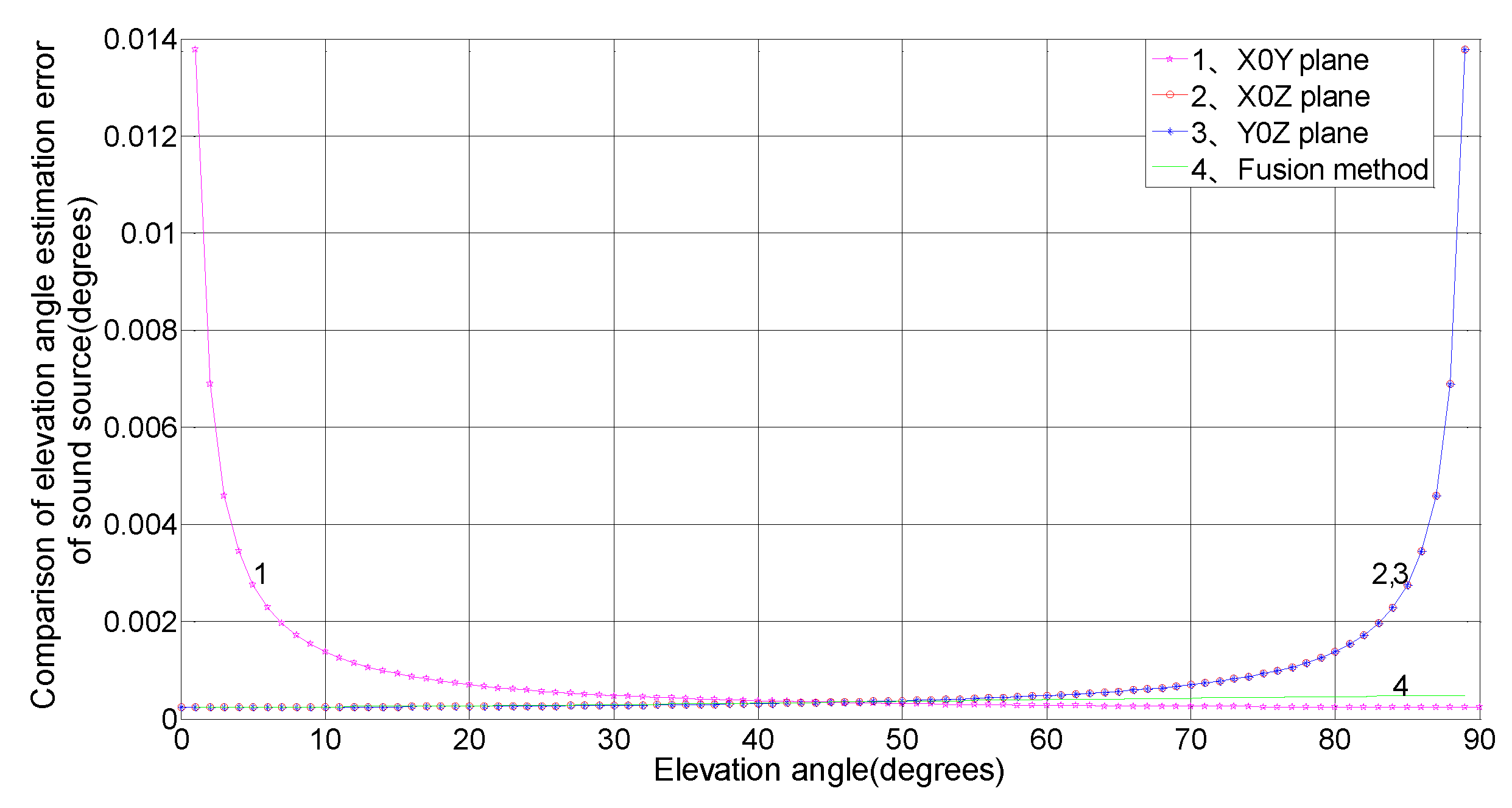
The measurement precisions of the elevation angle for the X0Y, X0Z, and Y0Z planes and the three-plane array were simulated, compared, and analyzed. The results are shown in Figure 2 for an array element spacing $a$ of 1 m, a sound velocity $c$ of 340 m/s, a time-delay estimation error value ${\sigma }_{\tau }$ of 1 μs, and an arbitrary planar elevation angle ranging from 0° to 90°.

As shown in Figure 2, the elevation angle estimation error ${\sigma }_{\theta }$ is greatly influenced by itself, where the error measured in the X0Y plane decreases with increasing elevation angle $\theta$, and the error measured in the X0Z and Y0Z planes increases with increasing elevation angle $\theta$. Through the three-plane fusion algorithm, the error is weakly influenced by itself, with an error of less than 0.001°. In conclusion, the fusion algorithm has advantages over a single-plane microphone array in elevation angle measurement precision, and its stability is obviously better than that of the X0Y, X0Z, and Y0Z plane approach.

4.2.2. Analysis of the Horizontal Angle Measurement Precision of the Sound Source

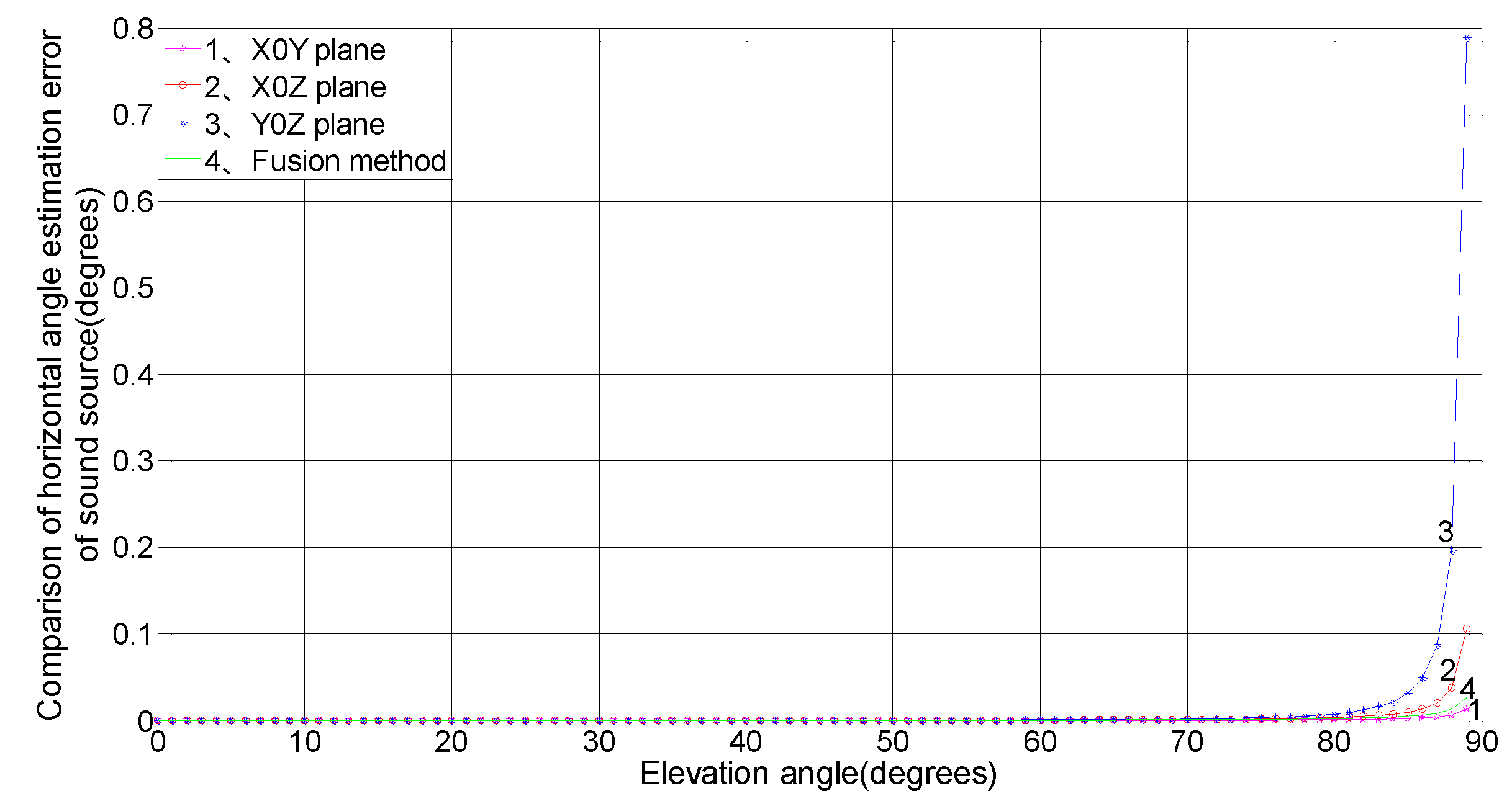
The measurement precisions of the horizontal angle for the X0Y, X0Z, and Y0Z planes and the three-plane array were simulated, compared, and analyzed. The result is shown in Figure 3 for an array element spacing $a$ of 1 m, a sound velocity $c$ of 340 m/s, a time-delay estimation error value ${\sigma }_{\tau }$ of 1 μs, a horizontal angle of 45°, and an arbitrary planar elevation angle ranging from 0° to 90°.

Figure 3 shows that when the elevation angle $\theta$ is between 0–80°, the horizontal angle estimation error ${\sigma }_{\phi }$ changes little. However, when the elevation angle $\theta$ is at an extreme angle of 80° to 90°, the error measured in the Y0Z plane obviously increases with elevation angle $\theta$. The error measured in the X0Z plane also rises sharply with increasing elevation angle $\theta$, reaching approximately 0.1°, which is second only to that of the Y0Z plane. The errors for the X0Y plane and the three-plane array are smaller at less than 0.05° and are almost unaffected by changes in the elevation angle $\theta$. In summary, when the elevation angle $\theta$ is large, the three-plane fusion algorithm is slightly inferior to the X0Y plane approach in horizontal angle measurement precision; when the elevation angle $\theta$ is extreme, the measurement precision of the fusion algorithm is better than both the X0Z and Y0Z plane results.

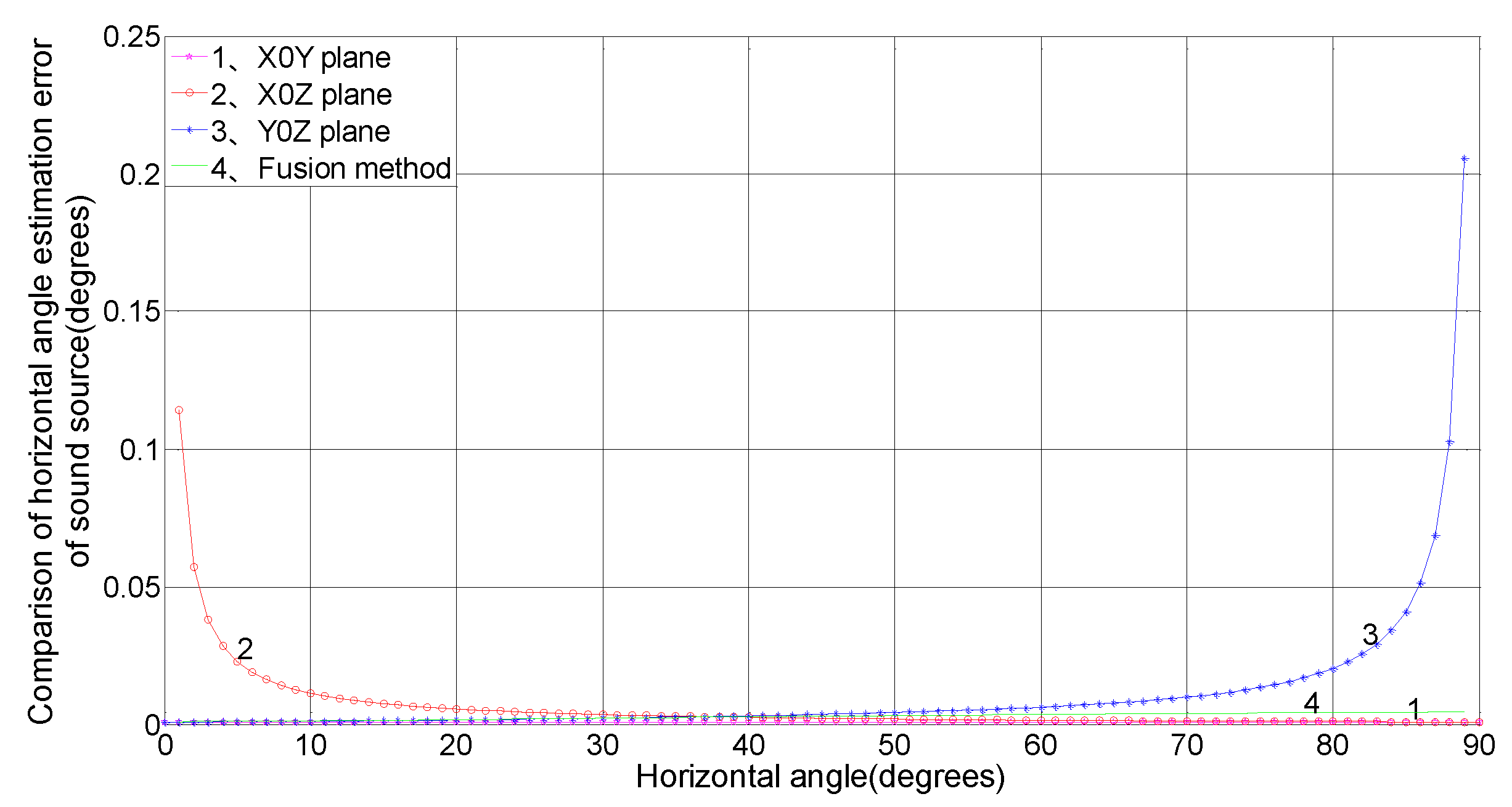
Results are shown in Figure 4 for an array element spacing $a$ of 1 m, a sound velocity $c$ of 340 m/s, a time-delay estimation error value ${\sigma }_{\tau }$ of 1 μs, an elevation angle $\theta$ of 75°, and an arbitrary planar horizontal angle ranging from 0° to 90°.

Figure 4 shows that the horizontal angle estimation error ${\sigma }_{\phi }$ measured in the X0Y plane does not influence itself. The error measured in the X0Z plane decreases with its own increase, and the error in the Y0Z plane increases with its own increase. The error measured for the three-plane array shows little change with a change in the horizontal angle $\phi$, and the error ${\sigma }_{\phi }$ is less than 0.001°. In summary, the three-plane fusion algorithm has distinct advantages in horizontal angle measurement precision over a single-plane array, and the stability is significantly better than that of the X0Z and Y0Z planes.

4.3. Influence of Time-Delay Estimation Error on Sound Source Localization Performance

The influence of the time-delay estimation error on the localization performance of the sound source is studied. Through simulation, the relationship between the time-delay estimation error and the direction-finding precision is obtained. The time-delay estimation error ${\sigma }_{\tau }$ is between 1–100 μs, the array element spacing $a$ is 1 m, and the sound velocity $c$ is 340 m/s.

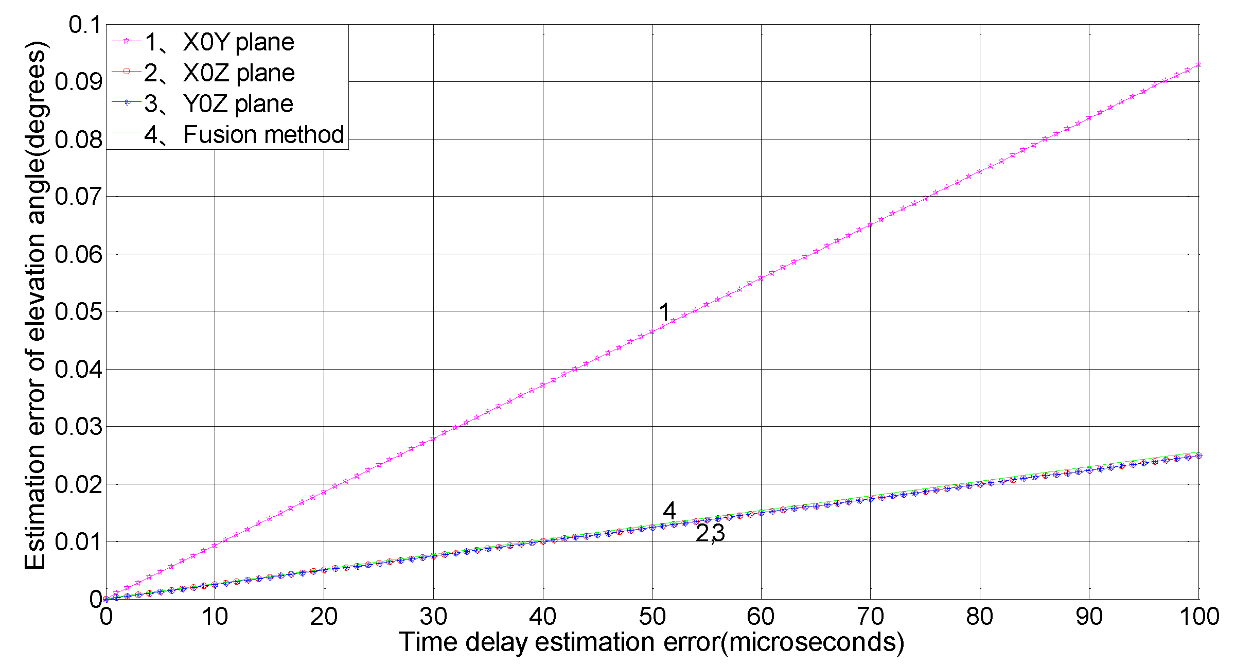
The relationship between the time-delay estimation error and the elevation angle measurement precision is shown in Figure 5 for an elevation angle $\theta$ of 15°.

Figure 5 shows that as the time-delay estimation error ${\sigma }_{\tau }$ increases, the elevation angle estimation error ${\sigma }_{\theta }$ measured in the X0Y plane shows the greatest increase. The X0Z and Y0Z measurement errors increase minimally, and the error of three-plane array is close to that of the X0Z and Y0Z planes, with a small increase. When the time-delay estimation error ${\sigma }_{\tau }$ is 100 μs, the error ${\sigma }_{\theta }$ is only 0.025°.

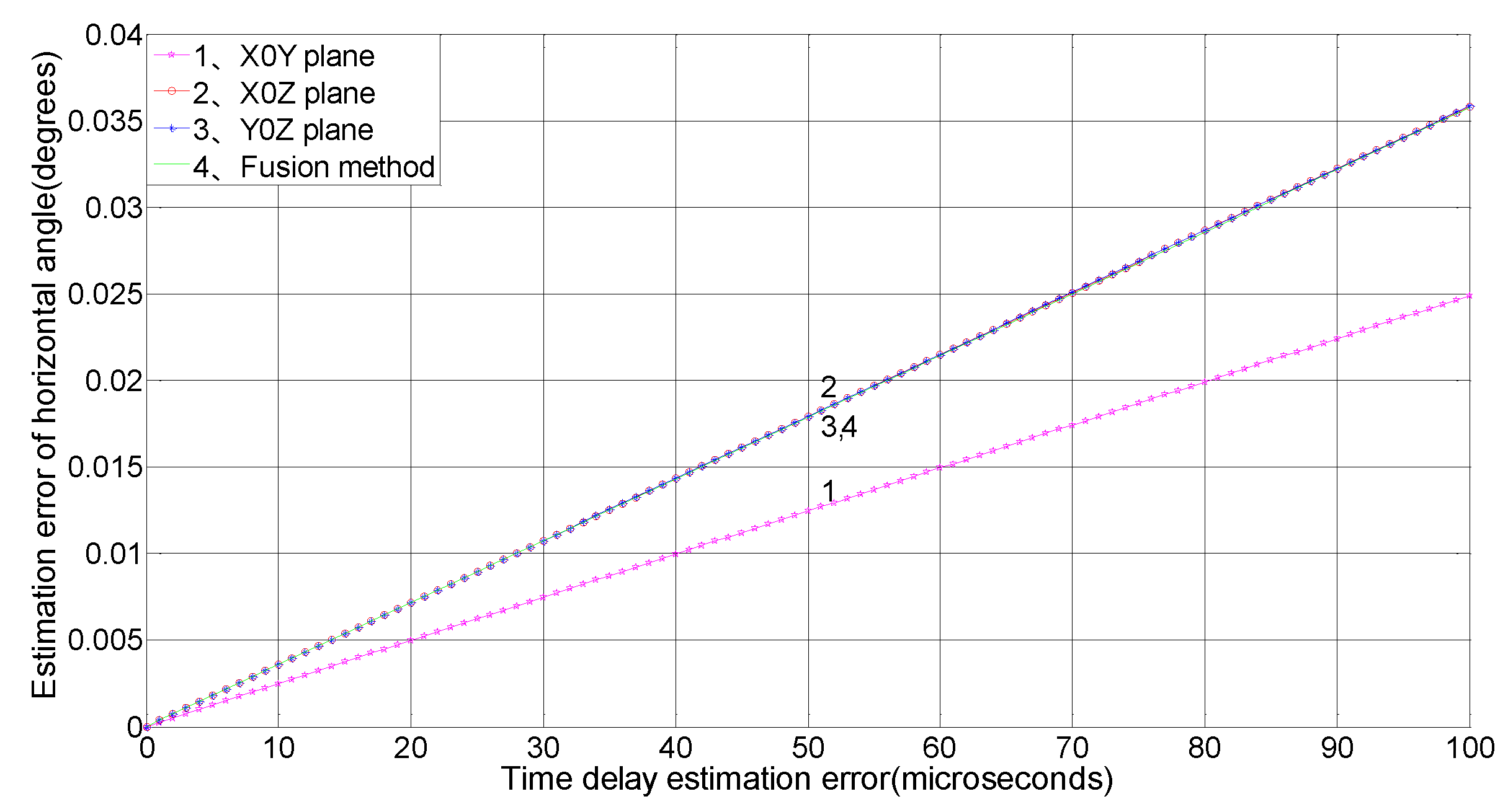
The relationship between the time-delay estimation error and the horizontal angle measurement precision is shown in Figure 6 for a horizontal angle $\phi$ of 45° and an elevation angle $\theta$ of 15°.

Figure 6 shows that as the time-delay estimation error ${\sigma }_{\tau }$ increases, the horizontal angle estimation error ${\sigma }_{\phi }$ shows the greatest increase in the X0Z plane. The error in the three-plane array is close to that of the Y0Z plane, and the error increase is large. When the time-delay estimation error ${\sigma }_{\tau }$ is 100 μs, the error ${\sigma }_{\phi }$ is approximately 0.036°, and the error ${\sigma }_{\phi }$ increase in the X0Y plane is minimized.

Figure 5 and Figure 6 show that the estimation error of angles measured by the single-plane and the three-plane array increase with the increasing time-delay estimation error, but relatively speaking, the three-plane fusion algorithm has a higher ranging precision and a more stable performance, and does not change drastically with changes in the time-delay estimation error.

5. Experimental Measurement Results and Analyses

For experimental measurements, this paper uses microphones to construct the sound source data acquisition system of a single-plane and a three-plane five-element microphone array, writing the program on the Keil5 software platform, using Flymcu to receive the serial port transmission data, and measuring six sets of relative time-delay values. The fusion algorithm is introduced, and the spherical coordinates of the sound source are calculated using time-delay values. Finally, several sets of indoor and outdoor experiments comparing the fusion algorithm with single-plane array and official radar chart data are performed.

5.1. Indoor Experiment

The indoor test site selected was the Acoustics Laboratory of Nanjing University of Information Science and Technology, Pukou District, Nanjing, and Bluetooth audio was used to simulate the sound source. The indoor experiment scene was shown in Figure 7.

In Figure 7, this experiment uses a pressure microphone, which has good omnidirectionality; its receivable signal has a bandwidth of 12 kHz. The predetermined position coordinates $(r,\theta ,\phi )$ are as follows: (2 m, 45°, 60°), (3 m, 15°, 45°), and (4 m, 75°, 30°). The experiment was performed with corresponding adjustment array element spacings of 0.5 m, 0.75 m, and 1.0 m. The results are shown in

Table 2. First experimental results.

Sound Source Spherical Coordinates	(2 m, 45°, 60°)
single-plane	(2.1298 m, 44.1055°, 56.7482°)
three-plane	(2.0840 m, 44.5317°, 57.8079°)

,

Table 3. Second experimental results.

Sound Source Spherical Coordinates	(3 m, 15°, 45°)
single-plane	(3.1045 m, 14.2482°, 43.9375°)
three-plane	(3.0729 m, 14.6057°, 44.0026°)

,

Table 4. Third experimental results.

Sound Source Spherical Coordinates	(4 m, 75°, 30°)
single-plane	(3.9104 m, 74.5260°, 28.5346°)
three-plane	(3.9570 m, 75.1745°, 29.3421°)

and

Table 5. Experimental data error rate in the three-plane array.

Experimental Data	Distance Error Rate/%	Elevation Angle Error Rate/%	Horizontal Angle Error Rate/%
first	4.20	1.04	3.65
second	2.43	2.63	2.22
third	1.08	0.23	2.19

.

As shown in Table 2, Table 3, Table 4 and Table 5, in the case of little indoor experimental environment noise and reverberation, the three-plane fusion algorithm—not the single-plane microphone array—has a higher sound source data precision compared with the theoretical data. Although there is a deviation, it is reasonable; thus, the data are stable and reliable.

According to Table 2, the ranging error of the fusion algorithm is 0.0840 m, while the error measured by the single-plane microphone array is 0.1298 m; therefore, the ranging precision is improved 1.5452-fold. The elevation angle error measured by the fusion algorithm is 0.4683°, while the single-plane error is 0.8945°; therefore, the elevation angle measurement precision is improved 1.9101-fold. The horizontal angle error measured by the fusion algorithm is 2.1921°, while the error measured by the single-plane microphone array is 3.2518°; thus, the horizontal angle measurement precision is increased 1.4834-fold.

According to Table 3, the ranging error of the fusion algorithm is 0.0729 m, while the error measured by the single-plane microphone array is 0.1045 m; therefore, the ranging precision is improved 1.4335-fold. The elevation angle error measured by the fusion algorithm is 0.3943°, while the single-plane error is 0.7518°; hence, the elevation angle measurement precision is improved 1.9067-fold. The horizontal angle error measured by the fusion algorithm is 0.9974°, while the error measured by the single-plane sound source array is 1.0625°; therefore, the horizontal angle measurement precision is increased 1.0653-fold.

According to Table 4, the ranging error of the fusion algorithm is 0.0430 m, while the error measured by the single-plane microphone array is 0.0896 m; therefore, the ranging precision is improved 2.0837-fold. The elevation angle error measured by the fusion algorithm is 0.1745°, while the single-plane error is 0.4740°; thus, the elevation angle measurement precision is improved 2.7163-fold. The horizontal angle error measured by the fusion algorithm is 0.6579°, while the error measured by the single-plane microphone array is 1.4654°; therefore, the horizontal angle measurement precision is increased 2.2274-fold.

As shown in Table 5, the error rate of the distance from the sound source to the center of the microphone array is approximately 3%, the elevation angle error rate is approximately 1.5%, and the horizontal angle error rate is approximately 2.5%. Due to the limitations of the experimental site, the maximum array element spacing is 1 m. Following the analysis of Section 4.3, the sound source localization error will be lower and more appropriate for displaying the advantages of the fusion algorithm when the array element spacing is increased appropriately.

In addition, taking the third experiment as an example, the performance of the algorithm is compared with references [24,26], and the results are shown in

Table 6. Comparison with the literature [24,26].

Data Source	Position S	Precision Compensation	Performance Analysis	Distance Error Rate/%	Angle Error Rate/%
fusion algorithm	Table 4	Equation (8)	Equation (12)	1.08	Max 2.19
Xu and Yang [24]	-	-	Section 3	Min 3.75	-
Su et al. [26]	Figure 8	joint optimisation	Figure 6	-	-

.

In Table 6, in terms of coordinate representation, Xu and Yang [24] performed poorly; although Su et al. [26] performed real-time 3D sound source mapping, they still did not know the location of the sound source; the fusion algorithm does this better. In terms of precision compensation, Xu and Yang [24] only stayed at the level of precision analysis, and there is no measure to improve the accuracy of sound source localization; Su et al. [26] provided a good initial guess for online optimization strategy through joint optimization. However, this measure is based on the sound source azimuth estimation algorithm. Therefore, when the sound source is at an extreme angle, it will still have a negative impact on the research of Su et al. [26]. In response to this impact, the accuracy compensation for sound source localization can be achieved using Equation (8). Although all three have analyzed the performance of the sound source localization algorithm, the experimental results show obvious differences among them. Since Su et al. [26] cannot determine the specific location of the sound source, the ranging and direction-finding error cannot be further given. When the acquisition card rate reaches one megabyte, the distance error rate measured by Xu and Yang [24] only reaches the minimum value of 3.75%; meanwhile, no measurement data is given in the measurement of angle. However, the distance and angle error rates measured by the fusion algorithm are 1.08% and 2.19% maximum, respectively. These error rates are still within the acceptable range when the elevation angle reaches an extreme angle of about 75°.

In summary, the sound source localization fusion algorithm of the three-plane five-element microphone array has higher precision, better stability, and an overall good performance in indoor experiments. By appropriately increasing the array element spacing in the three-plane array, compared with a single-plane array, one can measure the sound source position more accurately and stably.

5.2. Outdoor Experiment

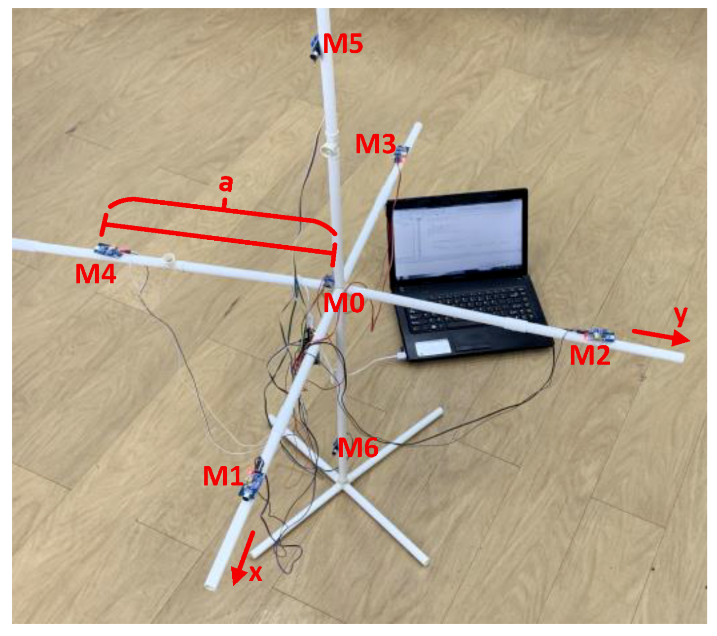
The outdoor experiment was carried out on the upper floor aisle of School of Electronic and Information Engineering, Nanjing University of Information Science and Technology. On this occasion, the target of sound source localization was thunder source point. The outdoor experiment scene is shown in Figure 8.

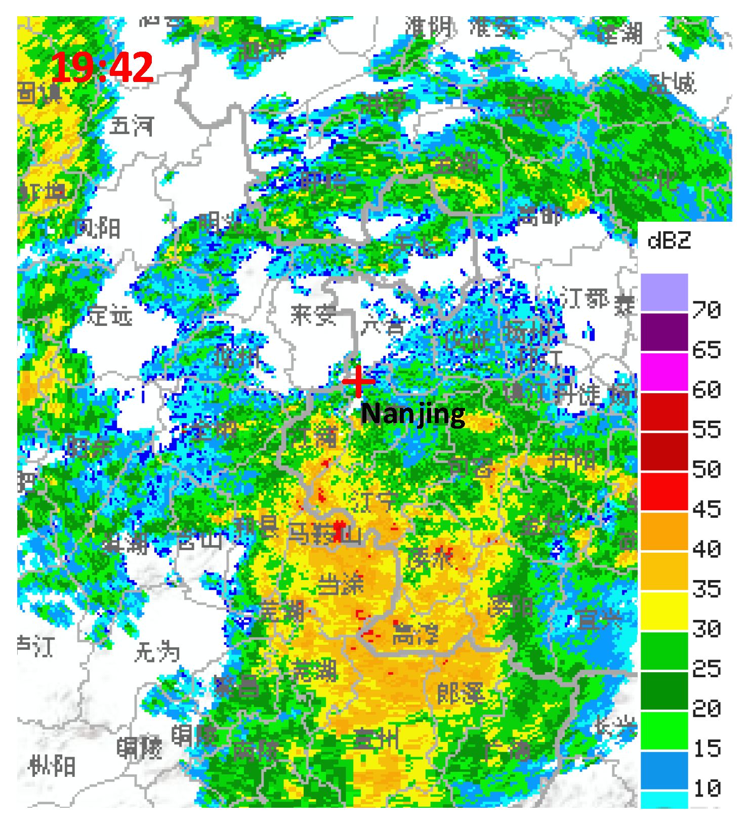
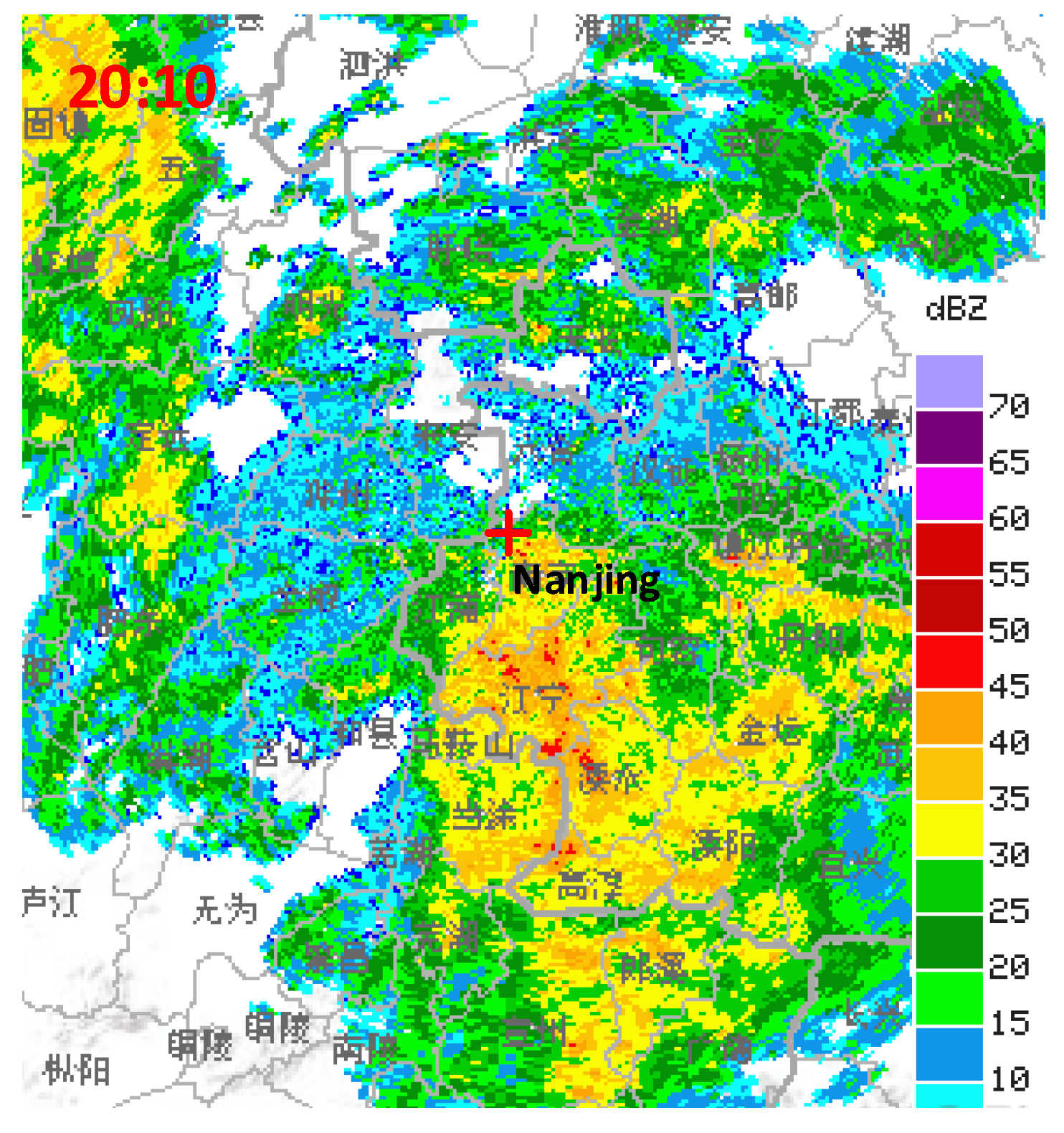
In Figure 8, the positive half of the x-axis and the y-axis of the three-plane five-element microphone array were respectively aligned in the south and east directions. With the help of the real-time data from the radar chart, the outdoor application effect of the fusion algorithm was analyzed. We set the array element spacing to 1.0 m and conducted two experiments to expect the algorithm to provide data feedback for thunderstorm cloud forecast warnings. The first experimental time was around 19:42 on 22 April 2019, and the data obtained by the fusion algorithm and the radar chart at this time are shown in

Table 7. First experimental results.

Data Source	Sound Source Spherical Coordinates
fusion algorithm	(4.2 km, 24.1°, −32.7°)

and Figure 9, respectively. The second experimental time was around 20:10 on the same day.

Table 8. Second experimental results.

Data Source	Sound Source Spherical Coordinates
fusion algorithm	(1.4 km, 78.5°, 46.9°)

showed the measured results of the fusion algorithm, and Figure 10 was the real-time radar chart. In addition, the red cross marked in Figure 9 and Figure 10 was the position of the measurement point.

In Table 7, the coordinates of the thunder source measured by the fusion algorithm were (4.2 km, 24.1°, −32.7°), the thunder source was about 32.7° west–south, and the elevation angle was relatively small, reaching 24.1°. In addition, the thunder source was 4.2 km away from the array center. This indicated that at around 19:42, the unexpected data was measured by the microphone array due to interference from the external environment, and no thunder source occurred in the upper area of the array. In Figure 9, the radar echo intensity was about 10 dBZ, indicating that a small amount of charge was accumulated in the cloud layer above the array, and no thunderstorm cloud existed. In summary, at 19:42 on 22 April 2019, there was no thunder source generated at the outdoor test point, and the real-time measurement result of the radar chart was consistent with the results obtained by the fusion algorithm, indicating that the method has better application effect. Besides, based on the data of 4.2 km and −32.7°, we can speculate that the thunderstorm cloud should be active nearby, which is likely to move from the southwest toward the test point.

In Table 8, the thunder source point coordinates measured by the fusion algorithm were (1.4 km, 78.5°, 46.9°). The thunder source was about 46.9° south by east, and it was only 1.4 km away from the array. In particular, the elevation angle was 78.5°, which was almost perpendicular to the z-axis. At this time, it is considered that the thunder source had occurred in the upper area of the array. At this point, in Figure 10, the radar echo intensity exceeded 40 dBZ, indicating that a large amount of charge was accumulated in the cloud layer above the array, and there was indeed a thunderstorm cloud. In summary, at 20:10 on 22 April 2019, the thunder source was generated over the test point, and the measurement results of the radar chart were consistent with the results obtained by the fusion algorithm. This is a good illustration of the effectiveness of the algorithm, and this experiment also verified the prediction of the previous experiment.

The fusion algorithm performs well in outdoor experiments, and the data measured by the algorithm can be consistent with the official radar data, reflecting its good overall performance.

5.3. Contrast Experiment

In order to further verify the effectiveness of the fusion algorithm, we compared with the literature [33]. Since the fusion algorithm and literature [33] are based on the seven-element stereo microphone array model, it is feasible to use the time-delay data measured by the same array shown in Figure 8 for comparative analysis.

To explore the extent to which the sound source is at an extreme angle to the negative impact of sound source localization performance, the sound source we selected is at (1.6 m, 2.7 m, 1 m), which matches the literature [33]. In addition, the spacing of the array elements was set to 0.4 m to match the experiment conducted in the literature [33] on 2 April 2018. At this time, the theoretical elevation angle of the sound source reaches 17.67°, which is an extreme angle and can verify the effectiveness of the fusion algorithm. The measured results are shown in

Table 9. Contrast experimental data.

Data Source	Coordinates /m	Distance Error Rate/%	Elevation Angle Error Rate/%	Horizontal Angle Error Rate/%
fusion algorithm	(1.5633, 2.6874, 1.0492)	0.38	5.52	0.78
Yang et al. [33]	-	3.89	7.95	0.66

.

As can be seen from Table 9, the distance error rate of the data measured by the fusion algorithm was far less than that measured by Yang et al. [33], and the error rate of the elevation angle was also slightly less than that measured by Yang et al. [33]. Although the error rate of the horizontal angle was slightly larger than that measured by Yang et al. [33], on the whole, the ranging and direction-finding performance of the fusion algorithm is better than that of the method proposed by Yang et al. [33].

From the perspective of commonality, both algorithms can locate the sound source; similarly, the difference between the two is also obvious. From Equations (20), (23), and (30) in the study of Yang et al. [33], it can be seen that the method proposed by Yang et al. [33] is affected by the sound source at an extreme angle. For example, when the elevation angle is close to 90°, the estimation error of the horizontal angle in Equation (20) is close to infinity, which is undoubtedly not expected. Assuming that the theoretical elevation angle of the contrast experiment is less than 10°, the error rate of data measured by Yang et al. [33] will rise sharply. On the contrary, the introduction of fusion algorithm can better solve this problem.

6. Conclusions

In this paper, a three-plane five-element microphone array model is constructed using seven microphones. In particular, the sinusoids and cosines of two elevation angles are introduced into the spherical coordinates of the sound source as composite weighted coefficients, and a sound source localization fusion algorithm for a three-plane, five-element microphone array is proposed. Finally, the effectiveness of the algorithm is verified by indoor, outdoor, and contrast experiments. In particular, with the official radar data, it is compared with the algorithm, and a good consistency result is obtained.

The three-plane microphone array has the ability to locate a sound source in the whole space, effectively solving the problem of a single-plane array, which easily blurs the measured sound source position. The fusion algorithm reduces not only the influence of azimuthal changes on ranging and direction-finding precision, but also influences the time-delay estimation error on localization performance, which fully reflects the advantages of the fusion algorithm.

The sound source localization fusion algorithm provides a more effective solution to reduce the negative impact of the sound source at an extreme angle on localization performance. In addition to being used for indoor and outdoor sound source location detection, the proposed algorithm can also be used to track the moving path of the thunderstorm cloud. This gives a more comprehensive data supplement for thunderstorm cloud forecast warnings, which is impossible for the current sound source localization algorithm. It should be noted that the proposed algorithm was based on the single microphone array model. Some studies believe that sound source localization based on an array group composed of multiple microphone arrays can improve the ability to monitor the location of a sound source using the network. Further work is recommended to verify this process.

From the practical application point of view, based on the three-plane five-element microphone array for the sound source localization fusion algorithm, the time-delay value can be fully utilized to detect the location of the sound source. In particular, the algorithm can be used for the array itself to check for faulty microphone damage, specifically which microphone is damaged; even after a microphone is damaged, it can still obtain sound source orientation data by using a single-plane five-element array. These are not realized by the seven-element microphone array. Of course, sound source localization technology still calls for further improvement. The practice of transferring experiments to harsh environments for performance testing requires further implementation.

References

- Man, Z.; Qian, W.; Ren, K.; Koutsonikolas, D.; Su, L.; Yanjiao, C. Dolphin: Real-Time Hidden Acoustic Signal Capture with Smartphones. IEEE Trans. Mob. Comput. 2019, 18, 560–573. [Google Scholar]
- Jena, D.P.; Panigrahi, S.N. Automatic gear and bearing fault localization using vibration and acoustic signals. Appl. Sci. 2015, 98, 20–33. [Google Scholar] [CrossRef]
- Chan, Y.T.; Ho, K.C. A simple and efficient estimator for hyperbolic location. IEEE Trans. Signal Process. 1994, 42, 1905–1915. [Google Scholar] [CrossRef]
- Zilong, Z.; Yichao, R.; Jing, Z.; Longjun, D.; Lianjun, C.; Xin, C.; Ruishan, C. A New Closed-Form Solution for Acoustic Emission Source Location in the Presence of Outliers. Appl. Sci. 2018, 8, 949. [Google Scholar]
- Trung-Kien, L.; Ho, K.C.; Trung-Hieu, L. Rank Properties for Matrices Constructed from Time Differences of Arrival. IEEE Trans. Signal Process. 2018, 66, 3491–3503. [Google Scholar]
- Gan, R.Z.; Feng, B.; Sun, Q. Three-Dimensional Finite Element Modeling of Human Ear for Sound Transmission. Ann. Biomed. Eng. 2004, 32, 847–859. [Google Scholar] [CrossRef]
- Vanthornhout, J.; Decruy, L.; Wouters, J.; Simon, J.Z.; Francart, T. Speech Intelligibility Predicted from Neural Entrainment of the Speech Envelope. J. Assoc. Res. Otolaryngol. 2018, 19, 181–191. [Google Scholar] [CrossRef]
- Fleury, V.; Davy, R. Analysis of jet–airfoil interaction noise sources by using a microphone array technique. J. Sound Vib. 2016, 364, 44–66. [Google Scholar] [CrossRef]
- Song, Y.L.; Lu, H.C.; Jin, J.M. Sound wave separation method based on spatial signals resampling with single layer microphone array. Acta Phys. Sin. 2014, 63, 187–196. [Google Scholar]
- Tavakoli, V.M.; Jensen, J.R.; Christensen, M.G.; Benesty, J. A Framework for Speech Enhancement With Ad Hoc Microphone Arrays. IEEE-ACM Trans. Audio Speech 2016, 24, 1038–1051. [Google Scholar] [CrossRef]
- Xu, W.; Zhang, C.; Ji, X.; Hongyan, X. Inversion of a Thunderstorm Cloud Charging Model Based on a 3D Atmospheric Electric Field. Appl. Sci. 2018, 8, 2642. [Google Scholar] [CrossRef]
- Su, L.; Ma, L.; Song, W.; Sheng-Ming, G.; Li-Cheng, L. Influences of sound speed profile on the source localization of different depths. Acta Phys. Sin. 2015, 64, 024302. [Google Scholar] [CrossRef]
- Yook, D.; Lee, T.; Cho, Y. Fast Sound Source Localization Using Two-Level Search Space Clustering. IEEE Trans. Cybern. 2015, 46, 20–26. [Google Scholar] [CrossRef] [PubMed]
- Bai, M.R.; Chen, C.C. Application of convex optimization to acoustical array signal processing. J. Sound Vib. 2013, 332, 6596–6616. [Google Scholar] [CrossRef]
- Ma, W.; Liu, X. Improving the efficiency of DAMAS for sound source localization via wavelet compression computational grid. J. Sound Vib. 2017, 395, 341–353. [Google Scholar] [CrossRef] [Green Version]
- Xing, H.; He, G.; Ji, X. Analysis on Electric Field Based on Three Dimensional Atmospheric Electric Field Apparatus. J. Electr. Eng. Technol. 2018, 13, 1697–1704. [Google Scholar]
- Lylloff, O.; Fernandez-Grande, E.; Agerkvist, F. Improving the efficiency of deconvolution algorithms for sound source localization. J. Acoust. Soc. Am. 2015, 138, 172–180. [Google Scholar] [CrossRef] [PubMed]
- Chen, Z.; Zhu, H.; Mao, R. Research on localization of the source of cyclostationary sound field. Acta Phys. Sin. 2011, 60, 104304. [Google Scholar]
- Xu, W.; Feng, X.; Xing, H. Modeling and Analysis of Adaptive Temperature Compensation for Humidity Sensors. Electronics 2019, 8, 425. [Google Scholar] [CrossRef]
- Flanagan, J. Bandwidth design for speech-seeking microphone arrays. In Proceedings of the IEEE International Conference on Acoustics, Speech, Signal Processing, Tampa, FL, USA, 26–29 April 1985. [Google Scholar]
- Brandstein, M.S.; Silverman, H.F. A practical methodology for speech source localization with microphone arrays. Comput. Speech Lang. 1997, 11, 91–126. [Google Scholar] [CrossRef] [Green Version]
- Miao, F.; Yang, D.; Wen, J.; Lian, X. Moving sound source localization based on triangulation method. J. Sound Vib. 2016, 385, 93–103. [Google Scholar] [CrossRef]
- Liu, X.J.; Sun, C. A Sound Source Tracking Method Using Linear Prediction location. Audio Eng. 2010, 34, 62–66. [Google Scholar]
- Qinqi, X.; Yang, P. Sound Source location Algorithm and Error Analysis Based on Tetrahedral Array. Comput. Simul. 2013, 30, 296–299. [Google Scholar]
- Alon, D.L.; Rafaely, B. Beamforming with Optimal Aliasing Cancellation in Spherical Microphone Arrays. IEEE-ACM Trans. Audio Speech 2016, 24, 196–210. [Google Scholar] [CrossRef]
- Su, D.; Vidal-Calleja, T.; Miro, J.V. Towards real-time 3D sound sources mapping with linear microphone arrays. In Proceedings of the IEEE International Conference on Robotics & Automation, Singapore, 29 May–3 June 2017. [Google Scholar]
- Smith, J.O.; Abel, J.S. Close-Form Least-Squares Source Location Estimation from Range-Difference Measurements. IEEE Trans. Acoust. Speech Signal Process. 1988, 35, 1661–1669. [Google Scholar] [CrossRef]
- Alamedapineda, X.; Horaud, R.A. Geometric Approach to Sound Source Localization from Time-Delay Estimates. IEEE-ACM Trans. Audio Speech 2014, 22, 1082–1095. [Google Scholar]
- Beck, A.; Stoica, P.; Li, J. Exact and Approximate Solutions of Source Localization Problems. IEEE Trans. Signal Process. 2008, 56, 1770–1778. [Google Scholar] [CrossRef]
- Muravyov, S.; Zlygosteva, G.; Borikov, V. Multiplicative Method for Reduction of Bias in Indirect Digital Measurement Result. Metrol. Meas. Syst. 2011, 18, 481–490. [Google Scholar] [CrossRef] [Green Version]
- Xing, H.; Yan, Y. Detection of Low-Flying Target under the Sea Clutter Background Based on Volterra Filter. Complexity 2018, 2018, 1513591. [Google Scholar] [CrossRef]
- Parkhill, K.L.; Gulliver, J.S. Indirect measurement of oxygen solubility. Water Res. 1997, 31, 2564–2572. [Google Scholar] [CrossRef]
- Yang, X.; Xing, H.; Ji, X. Sound Source Omnidirectional Positioning Calibration Method Based on Microphone Observation Angle. Complexity 2018, 2018, 2317853. [Google Scholar] [CrossRef]
Figure 1.
Three-plane five-element microphone array.
Figure 2.
Comparison and analysis of the elevation angle estimation error of the sound source.
Figure 3.
Comparison and analysis of the horizontal angle estimation error of the sound source caused by an elevation angle change.
Figure 4.
Comparison and analysis of the horizontal angle estimation error of the sound source caused by a horizontal angle change.
Figure 5.
Relationship between the time-delay estimation error and elevation angle measurement precision.
Figure 6.
Relationship between the time-delay estimation error and horizontal angle measurement precision.
Figure 7.
The scene photo of indoor experiment.
Figure 8.
The scene photo of the outdoor experiment.
Figure 9.
Radar chart displayed at 19:42.
Figure 10.
Radar chart displayed at 20:10.