Article

Stochastic Traffic-Based Fatigue Life Assessment of Rib-to-Deck Welding Joints in Orthotropic Steel Decks with Thickened Edge U-Ribs

by
Junlin Heng
1,2,
Kaifeng Zheng
2,
Sakdirat Kaewunruen
1,* and
Charalampos Baniotopoulos
1
1
Department of Civil Engineering, School of Engineering, University of Birmingham, Birmingham B152TT, UK
2
Department of Bridge Engineering, School of Civil Engineering, Southwest Jiaotong University, Chengdu 610031, China
*
Author to whom correspondence should be addressed.
Appl. Sci. 2019, 9(13), 2582; https://doi.org/10.3390/app9132582
Submission received: 2 June 2019 / Revised: 21 June 2019 / Accepted: 21 June 2019 / Published: 26 June 2019
(This article belongs to the Special Issue Extreme Sciences and Engineering)

Abstract

:

Featured Application

The new findings highlight for the first time the fatigue life enhancement of rib-to-deck joints using the innovative thickened edge U-rib in a real application. It also brings an in-depth insight to the effect of lateral position on the fatigue life of rib-to-deck joints. The method in the article can be used as a reference for the research and design of orthotropic steel decks.

Abstract

Rib-to-deck (RD) joints in orthotropic steel decks (OSDs) are highly prone to fatigue cracking under heavy traffic. An innovative longitudinal rib, named the thickened edge U-rib (TEU), has been proposed to enhance the fatigue strength of RD joints and validated through model tests. However, more studies are still required on the effect of TEUs in real engineering applications. To this end, a typical OSD bridge in China has been investigated, based on the experimental results. In the analysis, a stochastic traffic model is employed to simulate the vehicle-induced fatigue actions comprehensively. The framework of the stochastic model is proposed by considering the randomness in both the vehicles and their lateral distribution. Then the traffic model is instantiated using standard truck models in conjunction with the codes of practice as well as the observed data. A multi-scale finite element model is later established to determine the stochastic stress responses, whereas the influence surface method is used to improve computational efficiency. In this study, Monte Carlo simulations have been carried out to derive the stress spectra for the RD joints at different critical locations. Based on the test data and the derived spectra, an engineering assessment has been performed to obtain the fatigue life of RD joints in OSDs with and without TEUs, respectively. The new findings show that the position of joints has a remarkable influence on the stress spectra of RD joints, which results in the notable difference in fatigue life of the joints. Further, the fatigue life of RD joints can be significantly prolonged by using TEUs, and the prolongation rates are varied from 141% to 161% depending on the calculation methods and traffic models used.

1. Introduction

Orthotropic steel decks (OSDs) have been extensively applied in steel bridges since the reconstruction efforts following the Second World War due to their excellent performance such as light self-weight, short construction period, high loading capacity, and large redundancy etc. [1]. The application of OSDs in China could serve as an illustrative example. Since the 1990s, OSDs have been successfully applied in long-span bridges to reduce the self-weight [2]. Meanwhile, OSDs are also widely employed in urban bridges to speed up the construction process and minimize the disruption of daily traffic. For many cases, the OSD has become a crucial symbol of modern steel bridges. Further, the OSD is also believed as the only deck system that can provide an engineering service life of more than 100 years [3].
In the OSD system, the deck plate is stiffened by the longitudinal ribs and transverse floor beams in orthogonal directions. Welding joints are extensively used to connect the components, which in turns result in the fatigue issue. Under the persistent loading-and-unloading process by vehicles, premature fatigue cracks are frequently observed in the rib-to-deck (RD) joints in OSDs after several decades of operation [4]. In some extreme cases in China, the deck could be poorly designed and fabricated, while the truck traffic can be heavy and of dynamic conditions [5,6]. Under this situation, fatigue cracks could even begin to initiate in the RD joints within only a few decades after construction [7,8]. Thus, the fatigue issue is now of particular concern, and may hinder the further application of OSDs.
Many attempts were undertaken by various researchers in dealing with this problem [9,10,11,12,13]. Among them, the thickened edge U-rib (TEU) has been proposed as a feasible way to enhance the fatigue strength of RD joints [13]. In TEUs, the thickness of the rib wall is remarkably increased at the edge, without a significant increase in the self-weight and fabrication costs. As a result, the allowable welding depth of RD joints could be improved a lot, which may in turns enhance the fatigue strength. A series of experimental studies [14,15] has been carried out on the OSDs with TEUs, including the tests of rib-to-deck specimens and OSD specimens. The results suggested that the fatigue strength of RD joints could be significantly improved using TEUs, which in turns may prolong the fatigue life of the joints. However, more investigations are now urgently required on the exact fatigue performance of the RD joints in OSDs with TEUs, by considering the situation of real engineering applications.
Generally, fatigue evaluation includes both fatigue strength (resistance) and fatigue action (loading effects) [16,17,18,19]. In OSDs, the vehicle load is the dominated factor inducing the fatigue damage in welding joints [15]. In most of the design codes and engineering specifications, vehicle loads are represented by the standard truck model with deterministic configurations [20,21,22]. The stress history in the welding joints could be solved using the truck model. Through the cycle-counting method [23], the stress history can be transformed into the equivalent stress range, which is then used in fatigue evaluation to reflect the fatigue action. Although the above approach is concise in engineering practices, it is not comprehensive enough to describe the highly complicated fatigue action. Thus, measurement-based traffic data have recently been employed in fatigue evaluation. Liu et al. [24] proposed a traffic model based on the measured data from a cable-stayed bridge in China. In the model, both the uncertainties in the vehicle and lane occupancy were considered. Yan et al. [25] employed the measured traffic data to calculate the stress response of welding joints in OSDs. In the study, the in-lane lateral position of vehicles was considered, but the differences in lane occupancy and vehicle type were ignored. Lu et al. [26] adopted the machine learning algorithm with a proposed traffic model to derive the stress spectra of welding joints in OSDs. Zhu et al. [27] applied the standard truck model with the measured weight in solving stress spectra, in which the Gaussian process surrogate model was used to improve efficiency.
In this paper, for the first time the fatigue life of rib-to-deck joints in OSDs with TEUs are investigated, considering the novel engineering application and stochastic traffic model. Through the fatigue tests, the effectiveness of TEUs has been validated in enhancing the fatigue strength of rib-to-deck joints. A typical OSD bridge in China has been selected as the prototype for further investigation based on the test results. In the analysis, a stochastic traffic model has been employed in deriving the vehicle-induced stress spectra to simulate the fatigue action comprehensively. The framework of the stochastic model is established considering the randomness in both the vehicle model and their lateral distribution. The traffic model is first instantiated using the standard truck models in the design codes including the Chinese Code for Design called ‘JTG’ (China) [20], Eurocode 1 (Europe) [21] and AASHTO (USA) [22]. After that, the observed traffic data is also used to construct the model. The multi-scale finite element (FE) model is established for the prototype bridge to transform the traffic into stress, and the influence surface method is applied to improve computational efficiency. Monte Carlo simulations are carried out with a large sample size (i.e., 107 in this study) to derive the stress spectra for RD joints at different critical locations. Finally, comparative assessment is conducted on the fatigue life of RD joints in OSDs with TEUs and those with conventional U-ribs (CUs). The method applied in this study could be referred to as a general approach in the fatigue design of OSDs. Meanwhile, the result demonstrates the effects of position of RD joints on fatigue life. Moreover, this study also highlights the advantage of OSDs with TEUs in improving the fatigue life of RD joints.

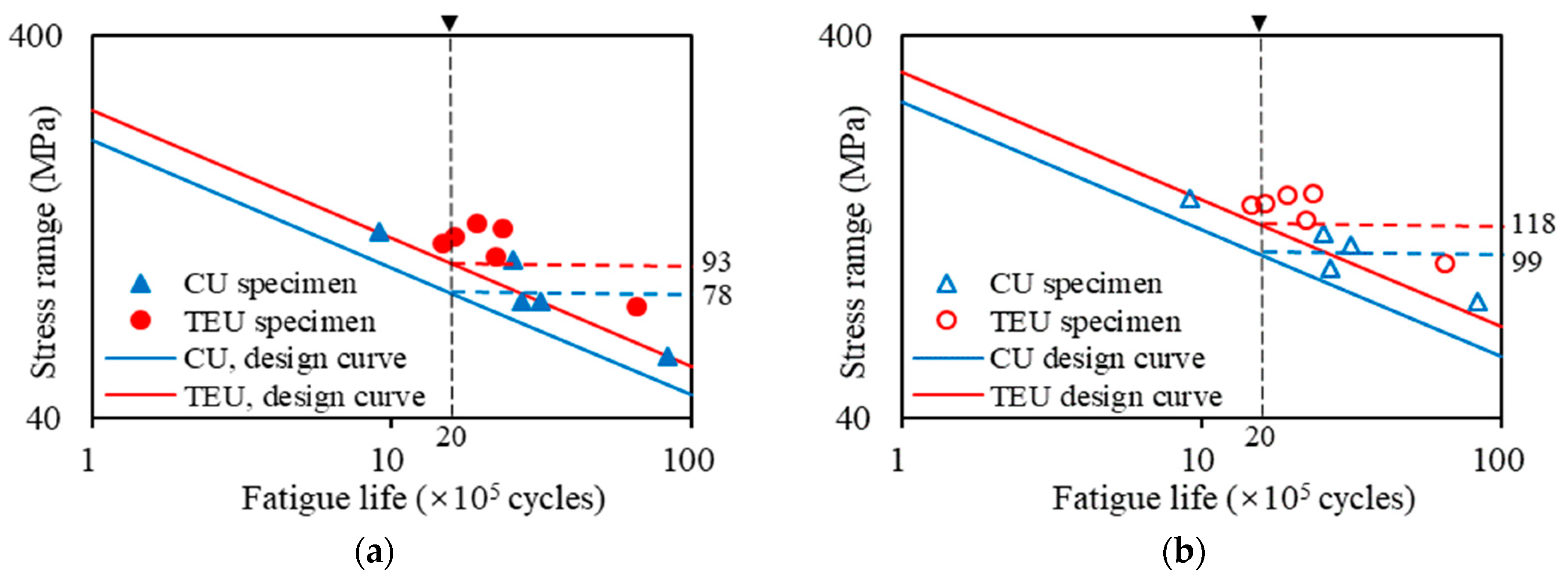
2. Comparative Fatigue Tests of Rib-to-Deck Joints

A series of fatigue tests have been carried out to investigate the fatigue strength of RD joints in OSD with TEUs [13,14]. A total of eleven specimens have been tested using the cyclic loads, including five CU specimens and six TEU specimens. Figure 1a shows the sectional view of the two types of specimen. Among the specimens, three CU specimens and four TEU specimens are tested with the central loading [13], as shown in Figure 1b. Further, the eccentric loading has been applied to two CU specimens and two TEU specimens [14], as shown in Figure 1c. The specimens are fabricated with the structural steel Q345qD [28] under the same welding process. As a common practice, each specimen consists of an 8 mm-thick U-rib and a 16 mm-thick deck plate, connected by the one-sided welding. As shown in Figure 1a, part of the rib wall (i.e., 2 mm) is left unwelded in order to avoid the weld-melt-through, which is harmful to the fatigue strength of joints. Compared with the CU specimens, the penetrated depth of the rib wall is increased from 6 mm to 10 mm (i.e., around 67%) in the TEU specimens. As a result, the weld leg length on the deck side is increased from 11 mm to 15 mm. Meanwhile, a smooth transition is achieved near the welding joint in TEU specimens, which could further reduce the local stress concentration in the joint.
The specimens are supported on a testing platform with bearing rubber plates to allow for rotation displacement. Constant amplitude loads have been applied by the actuator located at the centre of the specimen, as shown in Figure 1b. Dye penetration (DP) checks have been conducted to detect the crack during loading. In all the specimens, the same cracking pattern has been observed: the crack first initiates at the deck toe near the end and then propagates along both the length and thickness of the deck plate. Figure 2 shows the typical cracking pattern of the RD joint, including the result of DP checks during loading and the macro-section cut after the test. Since the crack occurs at the weld toe on the deck side in all the eleven specimens tested, the following investigation has been mainly focused on the deck toe-failure. Meanwhile, the “thickness penetration” criterion is employed to define the failure of the specimens: once the fatigue crack could be identified from both the top and bottom surfaces of the deck plate, the crack is regarded as a penetrated crack and failure of the specimen is achieved. Correspondingly, the number of loading cycles at the time is considered as fatigue life.
The stress range measured near the deck toe is taken as the fatigue strength since it is the initiation point of cracks. The fatigue strength of the specimens is expressed in terms of the nominal stress approach and the hot spot stress approach, respectively [29,30]. Due to the physical limitation on the size of strain gauges, the “0515” rule suggested by Niemi et al. [30] has been applied to determine the hot spot stress. In another words, the hot spot stress is determined through linear extrapolation based on the two reference points, which are 0.5t and 1.5t (where the parameter t is the plate thickness) away from the weld toe line, respectively.
Generally, the design of stress-life curves are derived under a specified survival probability and then used in the fatigue evaluation, in dealing with the variation in fatigue strength. As a result, the conservative result can be expected at the given survival rate. In this study, the design curves have been derived though the regression analysis based on the stress-life model shown in Equation (1):
l o g   N = l o g   C m · l o g   Δ σ
where N is number of the failure cycles; C and m are the material constant and power index; ∆σ is the applied stress range.
The method proposed by Hobbacher [29] has been applied in the regression, which employs the critical value at 95% survival probability. Since the experimental data are limited, the power index m is fixed as 3 [29]. The experimental data are listed along with the derived curves in Figure 3a,b, in terms of the nominal stress and the hot spot stress, respectively.
According to the result, the fatigue strength of RD joints in TEU specimens is notably higher than in CU specimens. In terms of the nominal stress, the FAT value (i.e., the design fatigue strength at 2 million cycles) is 78 MPa for CU specimens and 93 MPa for TEU specimens, respectively. Meanwhile, the FAT value in the hot spot stress is respectively 99 MPa and 118 MPa for the two types of specimens. Although the enhancement in fatigue strength has been validated for the OSD with TEUs through the test, further investigations are still urgently required on the application of TEUs in the real engineering project.

3. Engineering Background: The Prototype Bridge

A typical OSD bridge in Chengdu, China has been selected as the prototype for the investigation, as shown in Figure 4. The bridge consists of a 68 m-long main span and two 45 m-long side spans, which is a typical layout of urban steel bridges in China. The OSD system is divided by the transverse floor beams into 112 segments with similar configurations. The deck is 12.25 m-wide, carrying three lanes. Within each lane, there are 15 U-ribs located at different lateral positions, which are numbered from U1 to U15. For better illustration, the RD joints are represented by the numbers and a following subscript “L” or “R”, standing for the joint on the left or right sides of Uribs, respectively. Some other basic information could be found in Table 1.
Since the prototype bridge is on a major urban expressway with heavy traffic volume and a high proportion of trucks, the fatigue damage will accumulate with the time of operation and gradually lead to cracking in the RD joints. To this end, the OSD with TEUs have been applied in the design to prevent premature fatigue cracking in the joints. Investigations will be performed on the prototype bridge in order to compare the fatigue life of RD joints in the OSD with TEUs and the OSD with CUs.

4. Stochastic Traffic Model

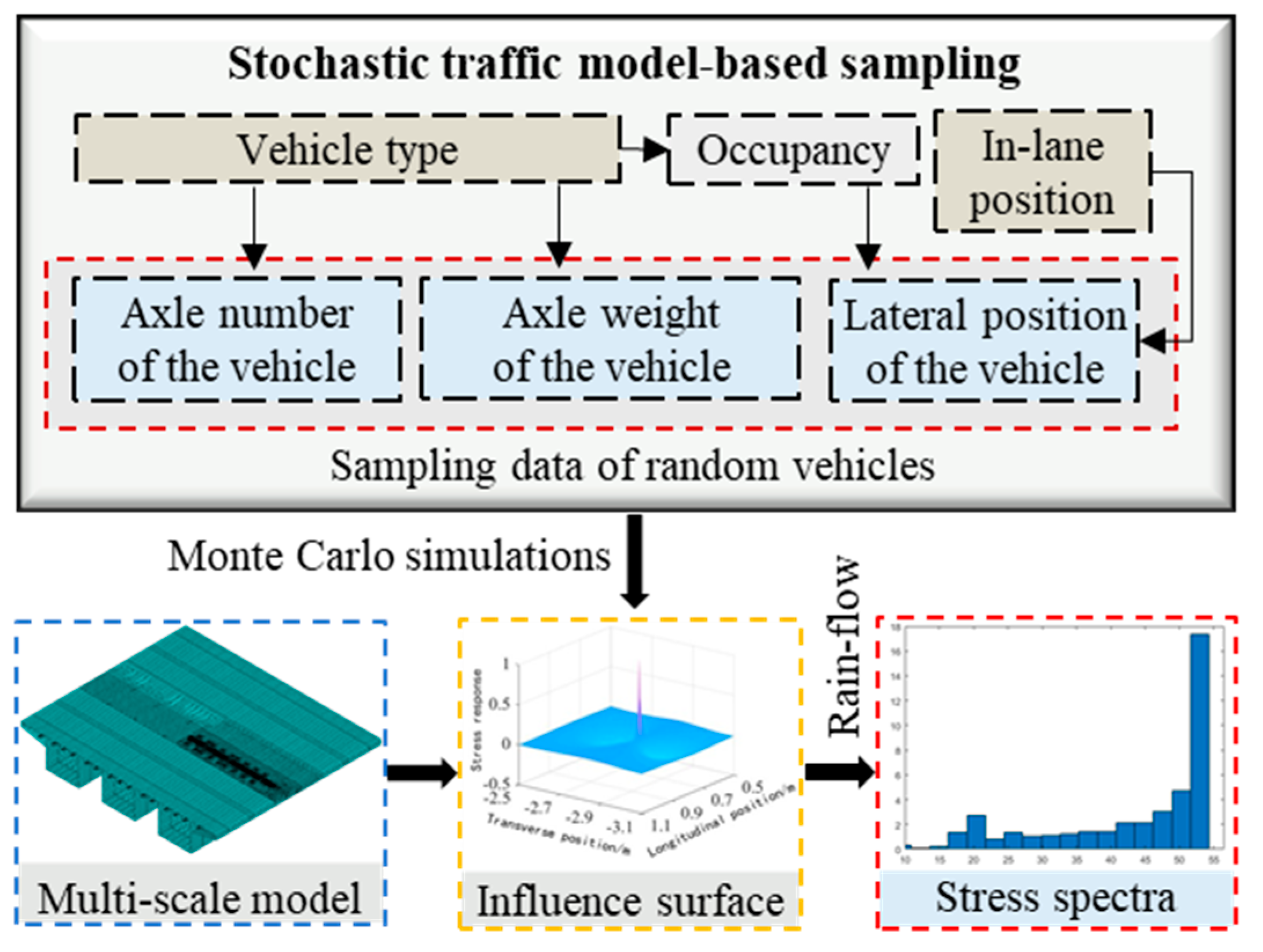
4.1. Framework of the Stochastic Traffic Model

In cases of fatigue evaluation, it is crucial to determine the stress spectra. With advanced monitoring systems, the stress spectra can be now directly established from measurements [31]. However, due to the limitations of budget and feasibility, the monitoring system could not yet be extensively applied [32]. Further, the spectra are not available at the design stage since it is not transferable for all the bridges. Alternatively, finite element (FE) analysis can be employed to derive the stress spectra in combination with the traffic model. As a result, the accuracy of the spectra largely depends on the rationality of the applied traffic model. In most of the codes and specifications, the vehicles are represented by the deterministic truck model. Several coefficients are usually applied to account for the randomness in traffic [20,21,22,23,24]. As a matter of fact, this method deviates from the random nature of vehicle loads, which may lead to inaccurate results [31].
Thus, a stochastic traffic model is proposed and applied in this study. The framework of the model is established by considering two primary elements: (1) the probabilistic model of vehicle properties; (2) the lateral distribution of vehicles. Since the stress response in RD joints are extremely sensitive to the configuration of the vehicle model [1,33], it is modelled in detail with the parameters including the axle number, axle spacing, axle weight, axle track and footprint. In the assumption, the lateral distribution is determined after both the occupancy rate and in-lane position. Table 2 summarizes the parameters defined in the framework, along with a brief description.

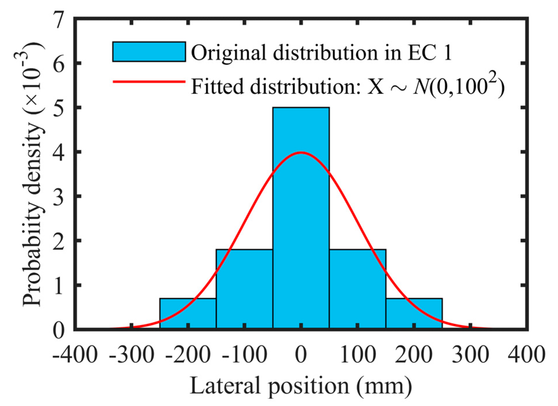
4.2. Data Source and Instantiation

After the framework is established, the parameters could be determined after two primary sources: (1) the existing traffic data in the publications such as design codes and guidelines; (2) the direct measurement by the monitoring systems installed on bridges, e.g., the weigh-in-motion system. Due to the lack of traffic data in the bridge site, the traffic model is first instantiated based on the fatigue truck models in the Chinese code JTG [20], European code Eurocode 1 (EC1) [21] and American code AASHTO [22]. Figure 5 shows the standard truck models proposed in the three codes. It is worth noting that no considerable difference could be found between the truck models in the JTG and EC1 except for the footprint. Also, the dynamic impactor factor is already considered in these two models. On the contrary, an additional impact factor of 1.15 should be applied when using the AASHTO truck since it is not included [22]. Furthermore, according to the measurements on the Williamsburg bridge and Bronx-Whitestone bridge [34,35], an extra amplification factor of 1.5 is suggested by the AASHTO in the fatigue evaluation of RD joints. Thus, when employing the AASHTO truck model, an overall amplification factor has been applied as 1.15 × 1.5 = 1.725.
According to the EC1 [21], 10% of the truck number in the slow lane can be used for the lane mainly occupied by light-weight cars, e.g., the fast lane in Figure 4. Under this assumption, the occupancy rate could be determined. In the AASHTO [22], the occupancy rate is related to the number of lanes available to trucks. Due to the traffic regulations and physic limitation, trucks seldom choose the fast lane when running on the three-lane highway, especially when heavily loaded. Thus, two lanes are assumed to be available to trucks for the prototype bridge, i.e., the middle lane and slow lane. As suggested by the AASHTO [22], the occupancy rate is determined as 85% for the slow lane and 15% for the middle lane. In the JTG [20], no specific provision could be found on the occupancy rate. As proposed by a supplementary document about the design of OSDs in China [36], the occupancy rate is kept the same as the value in the AASHTO. The occupancy rate in different traffic models is also listed in Figure 5.
Apart from the occupancy rate, the in-lane position is another essential factor in determining the lateral distribution of vehicles. In this aspect, no suggestion could be found in the AASHTO [22] while a distribution model is proposed in the EC1 [21] and adopted in the JTG [20]. Thus, the distribution has been employed for all three traffic models. As per the EC1 [21], the vehicle centre is considered as a random variable, discretely distributed over the width of lanes with the highest density in the lane centre, as shown in Figure 5. However, the lateral position is more likely a continuous variable that the vehicle can occur at every possible. Thus, the distribution has been fitted to the normal distribution using the maximum likelihood estimation [37], as shown in Figure 6. As a result, a zero mean and a standard deviation of 100 have been obtained.
Furthermore, the observed data [38] has also been used to instantiate the observation traffic model, as shown in Figure 7. The data were measured on a typical highway bridge in China, in which vehicles were classified into six groups according to the axle number, axle spacing, and axle weight. The brief description of each group is listed in Table 3, along with the lane occupancy rate.
Other details about the observed data could be found in the article [38]. Since the in-lane position was not provided, the distribution model previously discussed has been employed in the observation model. Meanwhile, since the data were measured in China, the footprint is kept the same as in the Chinese code JTG [20], i.e., 300 × 200 mm for the front axle and 600 × 200 mm for the rear axle. Similar to the AASHTO model, an extra impact factor of 1.15 should be applied when using the observation model in the analysis since the dynamic effect is not considered.

5. Influence Surface-Based Stress Spectra Analysis

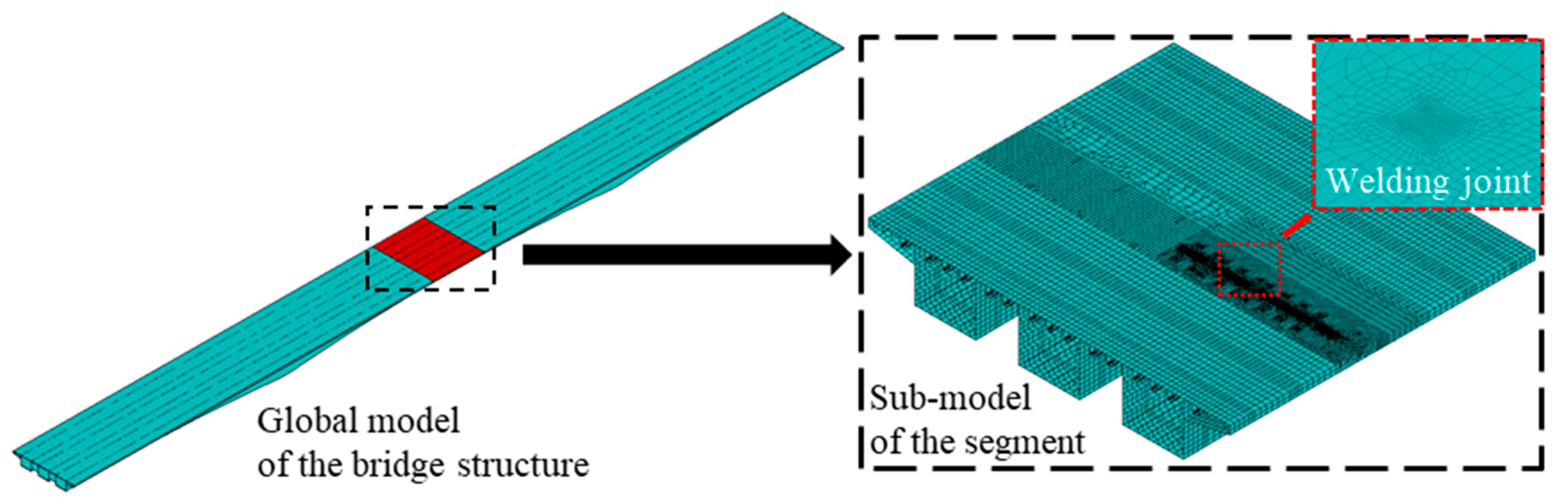
5.1. Multi-Scale Finite Element Model

Multi-scale finite element (FE) model is established for the prototype bridge using the ANSYS software [39] to derive the stress spectra under the traffic models, as shown in Figure 8. Due to the high similarity existed between the different segments of the OSD, the stress spectra are almost identical for the RD joints at the same lateral position [1,33]. To this end, the segment at midspan has been selected as a representative in the analysis.
The FE model consists of three parts: (1) the relatively coarse global model of the bridge structure, which is used to simulate the boundary condition on the segment of interests; (2) the highly refined local model in vicinity of the welding joints; (3) the refined sub-model of the segment, which serves as a meshing transition between the global model and the local model. In the global model, the 4-nodes shell element SHELL63 [40] has been applied. The sub-model and local model are established with the 8-nodes second order shell element SHELL93 [40] in order to ensure accuracy. The displacement of the sub-model is coordinated with the global model through the multi-point constraint (MPC) [41] on the boundaries, while the local model is connected to the sub-model by the sharing nodes. As a result, high accuracy could be achieved at an acceptable computational cost. It is worth stating that the element size is gradually refined to 2 mm in the local model, which meets the requirement of the hot spot stress approach [29,30]. As mentioned, the investigation is mainly focused on the deck toe-failure, i.e., cracking initiated at the weld toe on the deck side. Thus, the stress field in front of the deck toe is primarily concerned in the numerical investigation. In the FE model, all the shell elements are arranged in the middle plane, as suggested by Hobbacher [29]. In solving the hot spot stress, the extrapolation method and reference points have been kept the same as in the fatigue test, i.e., the “0515” rule. Since the local bending has influence mainly on the local nonlinear stress peak rather than the structural hot spot stress, the welds are not explicitly modelled. To this end, the reference points in the FE model have been selected through their distance to the intersecting line between the deck plate and rib wall.

5.2. Influence Surface-Based Solution

In the fatigue evaluation of welding joints, an essential step is to solve the full stress history under the vehicle model. Generally, the history induced by one vehicle should be solved with many solution steps, in which the vehicle is loaded at a series of adjacent locations in the longitudinal direction. Further, a large-size database of vehicles (i.e., 105) is often needed in deriving the stress spectra, even if the advanced Latino hyper sampling [42] is employed, which further escalates the computational complexity. Thus, the influence surface method has been employed to reduce the solving cost [1,25]. According to studies [1,33], the local stress in RD joints is highly sensitive to the location of wheel loads, and the influence of the loads is limited within one segment in length and two U-ribs in width. Based on this assumption, the loading area is selected, as shown in Figure 9.
The procedures of stress analysis are demonstrated in Figure 10, including the FE analysis, influence surface generation and stress history derivation. In the FE analysis, discrete stress responses have been solved by applying the unit nodal force on each node inside the loading area. Then, quadratic interpolation is used to construct the matrix of influence surface under the specific density, i.e., 2 mm in this study. After that, the influence surface of the unit wheel load could be easily generated through matrix operations on the influence surface of unit loads. Given the vehicle configuration and lateral position, the stress history induced by each wheel could be directly solved by vector operations. Finally, the full stress history of the vehicle could be calculated by the linear superposition of the wheel-based history over the time domain.
The approach shown in Figure 10 has been coded in the MATLAB [43], in combination with the stress result solved from the FE model. Figure 11a,b shows the influence surface of the unit nodal load in terms of the nominal stress and hot spot stress, respectively.
For a better illustration, the influence surface is unitised in Figure 10. The two results are highly similar with notable features: (1) a positive peak could be found in the vicinity of RD joints, which is extremely narrow; (2) near the positive peak there are two negative peaks, which are lower in the amplitude but much wider. Based on the above analysis, the stress history could be solved under the vehicle passing through different lateral positions. For illustration, the stress history with the highest response has been employed as the most critical history to compare the four traffic models. It can be found in Figure 4 that the joint U12L is prone to fatigue cracking since it is in the slow lane and close to the frequent loading position of wheels. Thus, the critical stress history of the U12L has been selected for the comparison, as shown in Figure 12a–d. It is worth stating that the stress history of one vehicle could be generated in less than 1/160 s by performing the influence surface-based analysis on a four-cores workstation, which may take more than 300 s using the same device (i.e., increased by almost 50,000 times in efficiency).
Unlike the standard truck models, the observation model takes into consideration the difference between vehicle groups as well as the uncertainties in axle weights of the vehicles within the same group. Thus, In the case of the observation model, the calculation is made using the most critical six-axles truck with the upper 97.7%th percentile value of axle weights [37]. The result shows that the stress history in RD joints is mainly determined by the axle number and axle weight. Further, no significant interaction could be found between the different axles. Among the three standard truck models, the AASHTO model results in the most conservative result, followed by the JTG model and then the EC1 model. In the case of the observation model, the result is similar to those solved with the standard truck models. It is worth stating that a considerable stress range could be found in the results solved with the AASHTO model and observation model (as shown in Figure 12c,d), demonstrating that the effect of front axles is not ignorable in fatigue evaluation of RD joints. Meanwhile, under all the four models, the stress history in the nominal stress and hot spot stress is highly similar, except for the difference in amplitude.

5.3. Monte Carlo-Based Spectra Derivation

Monte Carlo (MC) simulations are carried out to derive the stress spectra of the RD joints at various lateral locations. The derivation procedures are listed in Figure 13.
The Latin hypercube sampling (LHS) method [42] has been incorporated in the MC simulations to ensure better coverage over the whole distribution, which could in turns notably improve the sampling efficiency. As mentioned, a considerable number of samples is required in the MC simulations to simulate the stochastic traffic comprehensively. Thus, a large-size database is first generated based on the stochastic traffic model, i.e., 107 samples in this study. At the same time, the influence surface could be generated for the different RD joints. Then, the traffic database could be transformed into the database of stress history using the method illustrated in Figure 10. Finally, stress spectra could be established using the rain-flow method [29].

5.4. Fatigue Life Assessment

In the Eurocode 3 (EC3) [23], the three-stages stress-life (S-N) model is proposed, including two particular points, i.e., the transition point at five million cycles and the cut-out limit at 10 million cycles. Between the transition point and the cut-out limit, the power index m will change from three to five. Beyond the cut-out limit, infinite fatigue life could be expected for welding joints, indicating that the power index m is infinite. However, this only happens in the ideal situation when the pure constant amplitude loads are applied [29]. According to the fracture mechanics [44], the fatigue limit depends on both the material properties and the size of cracks, as shown in Equation (2):
Δ K t h = B Δ σ L π a i
where ΔKth is the fatigue threshold of the material, below which the crack will not grow; B is a constant related to the fatigue strength; ΔσL stands for the fatigue limit; ai is the crack size.
According to Equation (2), the fatigue limit will decrease with the increase in the crack size under the fixed fatigue threshold. Based on this assumption, the high-level stress ranges induced by heavy trucks will degrade the fatigue limit of joints with time. As a result, the stress ranges lower than the original limit will gradually contribute to fatigue damage [29]. On this end, the S-N should be expanded beyond 10 million cycles using the power index m = 5. Based on the above analysis, the S-N curves of RD joints have been modified, as shown in Figure 14a,b.
In this study, the linear damage accumulation rule is considered [45], as shown in Equation (3):
D = i = 1 n ( n i N i )
where D is the damage factor that failure; ni stands for the number of cycles corresponding to the stress range Δσi; Ni is the allowable fatigue life under the range Δσi.
Generally, the fatigue failure of welding joints is assumed when the damage factor D equals to 1.0 [20,22,23]. However, such consideration may lead to non-conservative results for OSDs, which is under the variable amplitude loading by different vehicles. Alternatively, the allowance of the damage factor D has been lowered to 0.5, as suggested by Hobbacher [29]. This factor is common in construction sector [46,47,48].
The fatigue life under the specific stress range could be calculated using the S-N curves, as shown in Equation (4):
N i = { ( Δ σ C / Δ σ i ) 3 · 2 × 10 6       Δ σ i > Δ σ D ( Δ σ D / Δ σ i ) 5 · 5 × 10 6         Δ σ i Δ σ D
where Δσc and ΔσD are the design fatigue strength at 2 million and 5 million cycles, respectively.
By setting the maximum damage factor as 0.5, the allowance of lifetime traffic volume could be solved through Equations (3) and (4).

6. Results and Discussion

6.1. Stress Spectra

As aforementioned, the joint U12L is exposed to a critical situation since it is located at the slow lane and close to the frequent loading position of wheels. Thus, the joint U12L is selected to investigate the difference in the stress spectra solved with the different traffic models. Since the spectra are highly similar in the nominal stress approach and hot spot stress approach, except for the amplitude, only the results in terms of the hot spot stress are listed, as shown in Figure 15. For clarity, the stress ranges with a small probability are truncated in Figure 15.
The result suggests that the stress ranges are highly scattered in the spectra, further illustrating that it is too concise to reflect the fatigue action in OSDs by the equivalent stress range solved with the deterministic truck model. At the same time, notable similarities could be found in the spectra solved under the three standard truck models. Although the critical joint U12L is selected, the low-level stress ranges (less than 15 MPa) still account for a considerable proportion in the spectra due to the randomness in the lateral position. As a result, it can lead to over-conservative results when only considering one or several critical lateral positions, as is the case in deterministic evaluation. It is also worth noting that the spectra solved by the JTG are more concentrated at the high-level ranges when compared with the one solved by the EC1, as shown in Figure 14a,b. The result could be explained by the only difference in footprints between the two models. Unlike the above two models, a local peak could be observed at the middle-level ranges (from 15 to 30 MPa) in the spectra solved by the AASHTO model. The front axle should be accounted for that, which further demonstrates its importance in the fatigue evaluation.
Meanwhile, compared with the results solved with the standard truck models, unique features could be observed in the spectra solve with the observation model: (1) the probability density of low-level ranges is relatively high; (2) the distribution is more even and continuous. The following factors could be accounted for: (1) six different groups of vehicles are considered in the observation model instead of a single truck; (2) the randomness in axle weight is considered in the model. As a result, the observation model could lead to a signifficant insight into the randomness in traffic, and it is applied in the following comparison.
Also, the joints U7L in the middle lane and U2L in the fast lane are selected to investigate the effect of occupancy rate on the spectra since the two joints are located at the same in-lane position as the joint U12L. The hot spot stress spectra are listed in Figure 16a,b, respectively.
The result indicates that the spectra of the joint U7L are similar to the spectra of the joint U12L, as shown in Figure 16a. According to Table 3, the difference in occupancy rate is small between the middle lane and slow lane for all the vehicles except the two-axles lightweight cars. Especially in terms of the five-axles and six-axles trucks, the differences in occupancy rate are only 10.6% and 5.8%, respectively. Meanwhile, the level of stress ranges in the joint U2L is generally lower than in the above two joints, as shown in Figure 16b. This result could be attributed to the following reason: although the total occupancy rate of the fast lane is the highest (i.e., around 42%), the proportion of heavier trucks in the fast lane is notably lower than in the other two lanes. In sum, due to the difference in the occupancy rate, the proportion of heavy trucks is higher in the slow lane and middle lane than that in the fast lane. As a result, the proportion of high-level stress ranges is significantly higher in the joints within the former two lanes than in the joints within the fast lane. Meanwhile, special care should be taken in fatigue design of not only the joints in the slow lane, but also those in the middle lane, since only a small difference exists in the occupancy rate of heavy trucks.
Further analysis has been carried out on the joint U13L, located at a different position in the slow lane, in order to investigate the effect of in-lane positions. The result is listed in Figure 17.
Although the joint U13L is also within the slow lane, the level of spectra is remarkably lower than in the joint U12L. The in-lane position could be the main reason: the joint U13L is almost laid at the centre of the lane, where the wheels could seldom act on. As a result, the level of ranges in the spectra is significantly low, even if the occupancy rate of heavy trucks is high in the slow lane. The analysis reveals a new finding that a prominent difference could be observed in the spectra of RD joints within the same lane, because of the influence of in-lane lateral position.

6.2. Fatigue Life Assessment

Based on the modified S-N curves and derived stress spectra, detailed investigations can be made to identify the fatigue life of RD joints in the novel OSD with TEUs and the traditional OSD with CUs. The four typical joints (i.e., U2L, U7L, U12L and U13L) have been used as the representatives since the effect of both the occupancy rate and in-lane position could be illustrated by the comparison on the four joints. Meanwhile, due to the lack of data on the traffic volume in the bridge site, the allowance of lifetime traffic volume has been chosen as the direct indicator. The results, which are unprecedented, are summarised in Table 4.
As aforementioned, remarkable differences could be observed in the stress spectra of RD joints at various lateral positions, which could further lead to the significant differences in the fatigue life of those joints. Two notable features could be found in Table 4: (1) with the same in-lane position, the joints within the middle lane or slow lane have a shorter fatigue life than within the fast lane; (2) within the same lane, the fatigue life is lower in the RD joints close to frequent loading position of wheels. Thus, the RD joint with the above two features can be regarded as the fatigue critical joint, to which special cares should be paid in fatigue design.
Since it is assumed in the JTG model and AASHTO model that heavy trucks seldom use the fast lane, the level of ranges is extremely low in the spectra of the joint U2L. As a result, the fatigue issue of the joint U2L could be almost ignored. In all the joints except the U2L, the JTG model leads to the most conservative result, followed by the AASHTO model, and then the EC1 model. It is also worth noting that the fatigue life is significantly higher in the results solved with the observation model than in the results solved by the standard truck models. This finding is due to the inclusion of lightweight cars in the observation model, which have the largest proportion but little contribution to the fatigue damage in RD joints. At the same time, the results also suggest a lower fatigue life could be determined by the hot spot stress approach when compared with the nominal stress approach, indicating the conservativeness of this approach.
Generally, the fatigue life of RD joints can be notably improved by the application of TEUs in OSDs. The prolongation rate is consistent under the three standard truck models, i.e., 141% in both the nominal stress approach and hot spot stress approach. Under the observation traffic model, the prolongation rate is from 141% to 143% in the nominal stress approach, and from 146% to 161% in the hot spot stress approach. In sum, this study for the first time demonstrates that the fatigue strength of RD joints can be effectively enhanced through the application of TEUs in OSDs, which in turn improves the fatigue life of RD joints under vehicle loads.

7. Conclusions

In this paper, a fatigue assessment has been performed for the first time on a novel orthotropic steel deck (OSD) with thickened edge U-ribs (TEUs) based on a stochastic traffic model. Through fatigue tests, the effectiveness of TEUs has been validated in enhancing the fatigue strength of rib-to-deck (RD) joints in OSDs. However, more investigations are still urgently required on the exact fatigue life of the joints in order to further validate the application of TEUs in engineering practices. On this end, comparative studies are conducted to determine the fatigue life of the RD joints in the OSDs with and without TEUs. A typical OSD bridge in China is selected as the prototype for the investigation. Since the vehicle load is the dominated factor inducing fatigue damage in OSDs, a stochastic traffic model is proposed and employed to highlight the uncertainties in vehicles. The framework of the stochastic model is idealised by considering both the vehicle properties and their lateral distribution. Then, the model is first instantiated through the standard truck models in the design codes, including the JTG (China), Eurocode 1 (Europe) and AASHTO (America). Further, measurement-based observation data have also been applied to construct the stochastic model, which can provide a better insight into the differences between, and within vehicle groups. At the same time, the multi-scale finite element (FE) model is established for the prototype bridge to transform the traffic model into the stress spectra required in fatigue evaluation. Influence surface method is used along with the FE analysis, which could improve the computational efficiency by almost 50,000 times. Monte Carlo simulations are then carried out to derive the stress spectra of RD joints at different lateral positions. Using the generated spectra, the influence of lateral positions has been illustrated in detail, including the lane type (fast, middle and slow) and in-lane position. Finally, based on the test data and derived spectra, a fatigue life assessment has been made for the RD joints in the OSDs with and without TEUs. According to this innovative study, the following conclusions could be drawn:
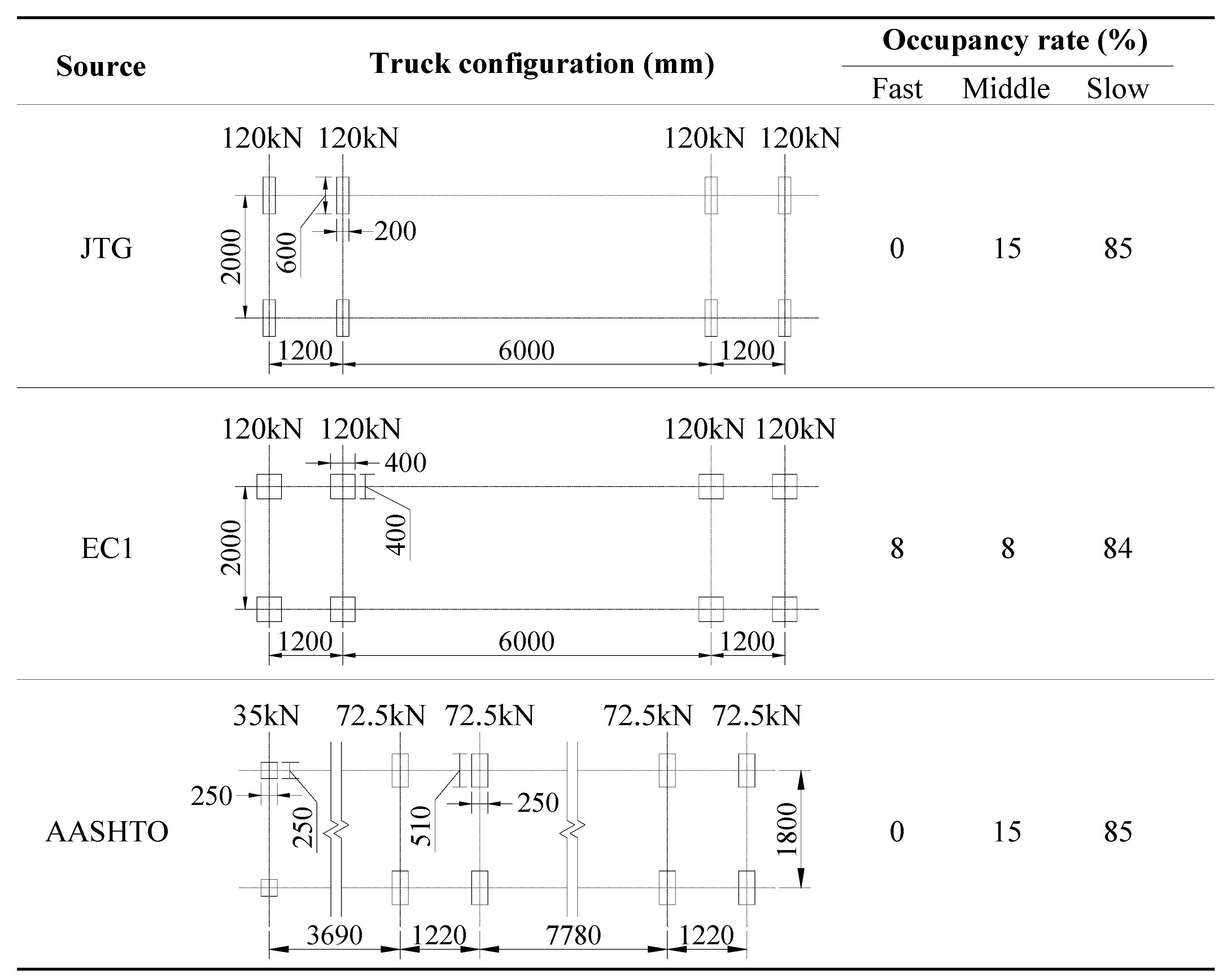
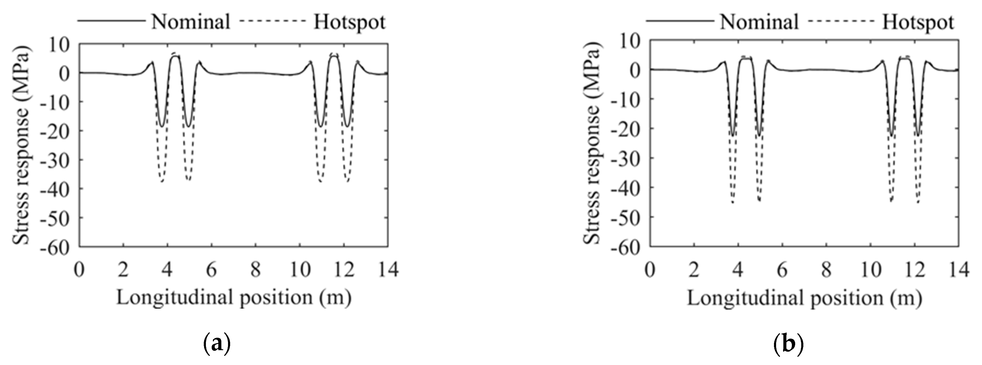
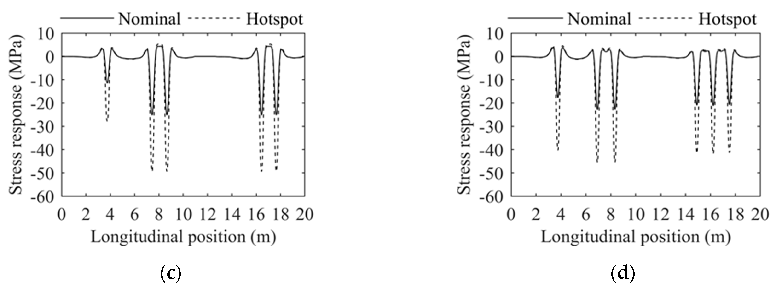
  • The four vehicle models are compared in terms of the critical stress history, including the standard trucks in the three codes and the six-axle critical truck in the observation model. The result shows that the standard truck in AASHTO will lead to the most conservative outcome, followed by the critical truck in the observation model, and then the standard trucks in the JTG, and at last the Eurocode 1. It is worth noting that, when using the AASHTO model and observation model, a notable stress range can be induced by the front axle, which is not negligible in fatigue evaluation.
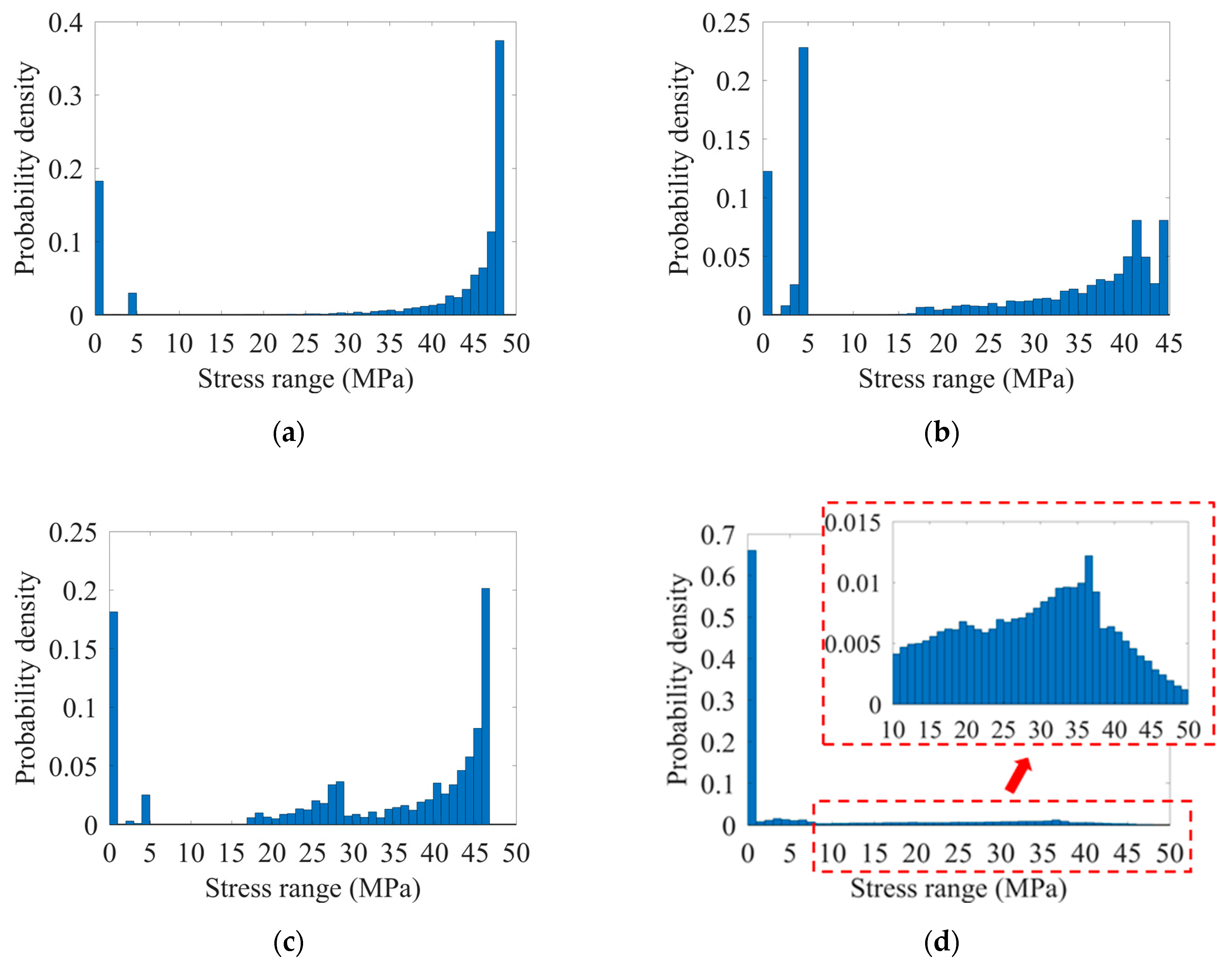
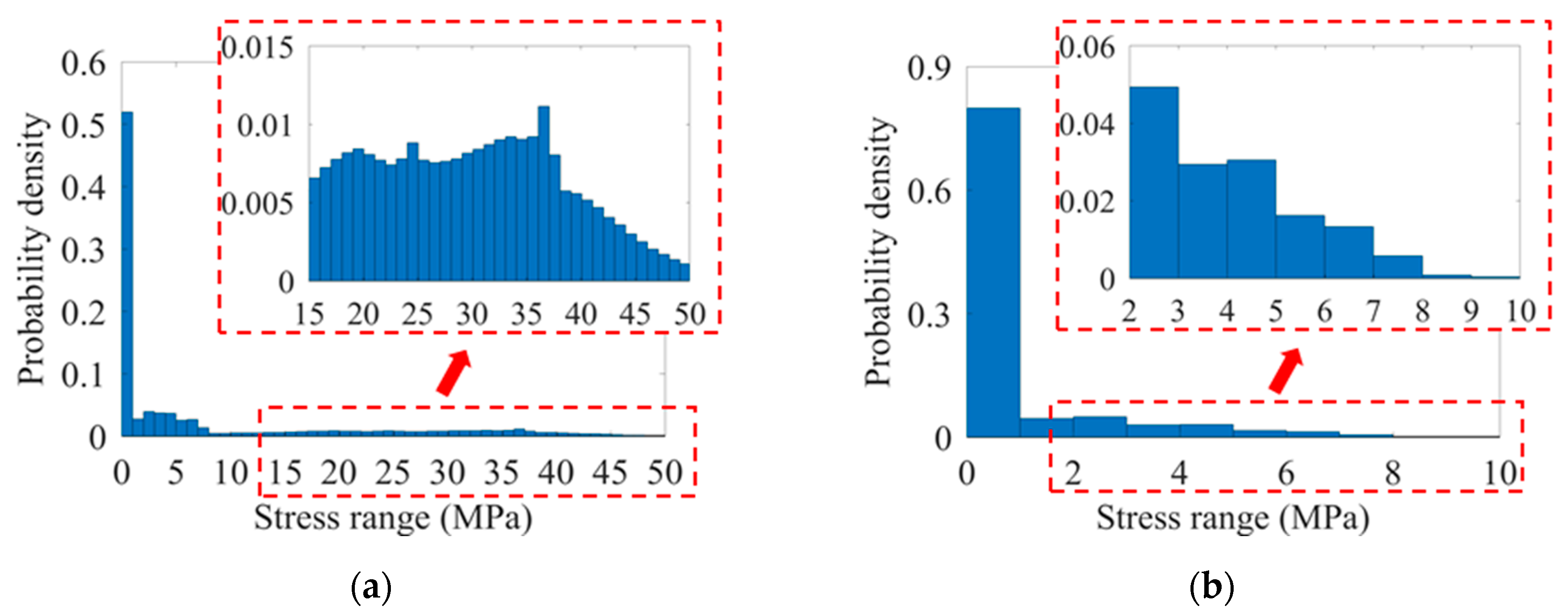
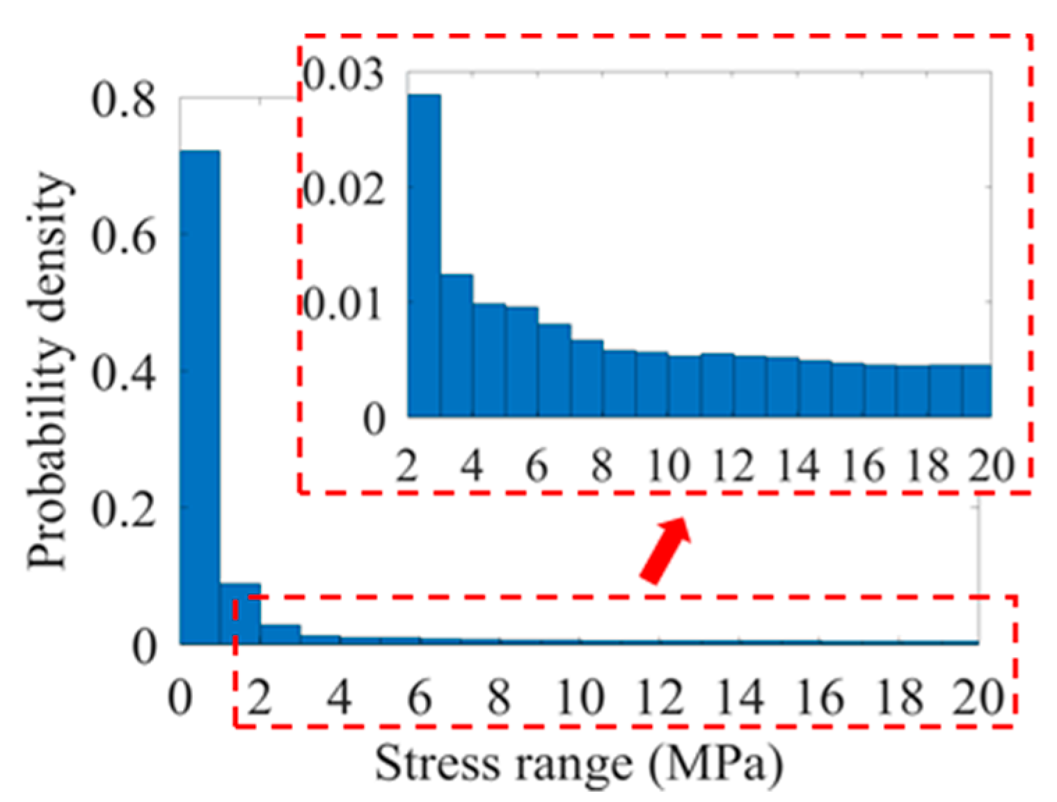
  • According to the solved spectra, the vehicle-induced stress ranges are widely distributed, illustrating it is oversimplified to describe the fatigue action by the equivalent stress range calculated with the deterministic truck model. Meanwhile, through a comparison between the spectra, it is proven that the observation model can bring an in-depth insight into the randomness in traffic since the model takes into consideration not only the randomness in lateral position but also the difference within and between vehicle groups.
  • The RD joints at various positions have been compared in terms of the stress spectra. Due to the lane preference, the proportion of heavy trucks is higher in the middle lane and the slow lane than in the fast lane. As a result, the proportion of high-level stress ranges is also higher in the spectra of the RD joints within the former two lanes. Meanwhile, comparisons are also made between the RD joints within the same lane. The result exhibits a remarkable difference in the stress spectra of the RD joints within the same lane, which is induced by the in-lane distribution of vehicles.
  • Based on the test data and the derived spectra, the fatigue life of RD joints at various locations can be determined. Overall, significant differences exist between the RD joints at different locations due to the lane preference and in-lane distribution. Meanwhile, the location of fatigue-critical RD joints has been identified through the results, i.e., the joint in the middle lane or the slow lane, and close to the frequent loading position of wheels. Thus, special care should be paid to this type of RD joint in fatigue design.
  • A comparison between the OSDs with and without TEUs has been performed in terms of the fatigue life of RD joints. Since the fatigue strength of RD joints could be effectively enhanced in OSDs with TEUs, the fatigue life of the joints could also be significantly prolonged. A consistent prolongation rate has been observed under the standard truck-based traffic models, which is 141% in both the nominal stress approach and the hot spot stress approach. Under the observation traffic model, the prolongation rate is between 141% and 143% in the nominal stress approach, and 146%–161% in the hot spot stress approach.

Author Contributions

Data collection, simulation, and writing—Original draft preparation, J.H.; supervision, project administration and funding acquisition, K.Z.; conceptualization, methodology and writing—Review and editing, S.K.; conceptualization, supervision and approve, C.B.

Funding

The research was funded by the National Natural Science Foundation of China (grant number: 51778536, Doctoral Innovation Fund Program of Southwest Jiaotong University (grant number: D-CX201701), the Zhejiang Department of Transportation (grant number: 10115066). The APC is sponsored by the University of Birmingham Library’s Open Access Fund.

Acknowledgments

The first author gratefully acknowledges financial support from China Scholarship Council and British Council during studying in the UK. Special thanks to European Commission for H2020-MSCA-RISE Project No. 691135 “RISEN: Rail Infrastructure Systems Engineering Net-work” (www.risen2rail.eu) [49].

Conflicts of Interest

The authors declare no conflict of interest.

References

  1. Connor, R.; John, F.; Walter, G.; Vellore, G.; Brian, K.; Brian, L.; David, L.M. Manual for Design, Construction, and Maintenance of Orthotropic Steel Deck Bridges; Federal Highway Administration: Washington, DC, USA, 2012. [Google Scholar]
  2. Zheng, K.; Heng, J.; Gou, C. The significant technical contribution made in the early development of orthotropic steel bridges in China. China Bridge 2015, 4, 10–15. (In Chinese) [Google Scholar]
  3. Fisher, J.W.; Roy, S. Fatigue of steel bridge infrastructure. Struct. Infrastruct. Eng. 2011, 7, 457–475. [Google Scholar] [CrossRef]
  4. Wolchuk, R. Lessons from weld cracks in orthotropic decks on three European bridges. J. Struct. Eng. 1990, 116, 75–84. [Google Scholar] [CrossRef]
  5. Remennikov, A.M.; Kaewunruen, S. A review of loading conditions for railway track structures due to train and track vertical interaction. Struct. Control Health Monit. 2008, 15, 207–234. [Google Scholar] [CrossRef]
  6. Kaewunruen, S.; Chiengson, C. Railway track inspection and maintenance priorities due to dynamiccoupling effects of dipped rails and differential track settlements. Eng. Fail. Anal. 2018, 93, 157–171. [Google Scholar] [CrossRef]
  7. Freimanis, A.; Kaewunruen, S. Peridynamic Analysis of Rail Squats. Appl. Sci. 2018, 8, 2299. [Google Scholar] [CrossRef]
  8. Zeng, Z. Classification and reasons of typical fatigue cracks in orthotropic steel deck. Steel Constr. 2011, 2, 9–15. (In Chinese) [Google Scholar]
  9. Sim, H.B.; Uang, C.M.; Sikorsky, C. Effects of fabrication procedures on fatigue resistance of welded joints in steel orthotropic decks. J. Bridge Eng. 2009, 14, 366–373. [Google Scholar] [CrossRef]
  10. Dung, C.V.; Sasaki, E.; Tajima, K.; Suzuki, T. Investigations on the effect of weld penetration on fatigue strength of rib-to-deck welded joints in orthotropic steel decks. Int. J. Steel Struct. 2015, 15, 299–310. [Google Scholar] [CrossRef]
  11. Nishida, N.; Sakano, M.; Tabata, A.; Sugiyama, Y.; Okumura, M.; Natsuki, Y. Fatigue behavior of orthotropic steel deck with both side fillet welds between deck and trough ribs. In Proceedings of the 68th JSCE Annual Meeting, Chiba ken, Japan, 4–6 September 2013. I-572. [Google Scholar]
  12. Zhang, Q.; Liu, Y.; Bao, Y.; Jia, D.; Bu, Y.; Li, Q. Fatigue performance of orthotropic steel-concrete composite deck with large-size longitudinal U-shaped ribs. Eng. Struct. 2017, 150, 864–874. [Google Scholar] [CrossRef]
  13. Heng, J.; Zheng, K.; Gou, C.; Zhang, Y.; Bao, Y. Fatigue performance of rib-to-deck joints in orthotropic steel decks with thickened edge u-ribs. J. Bridge Eng. 2017, 22, 04017059. [Google Scholar] [CrossRef]
  14. Heng, J.; Zheng, K.; Kaewunruen, S.; Zhu, J.; Baniotopoulos, C. Probabilistic fatigue assessment of rib-to-deck joints using thickened edge U-ribs. Steel Compos. Struct. 2019. under review. [Google Scholar]
  15. Chang, K.O.; Bae, D. Proposed revisions to fatigue provisions of orthotropic steel deck systems for long span cable bridges. Int. J. Steel Struct. 2014, 14, 811–819. [Google Scholar]
  16. Setsobhonkul, S.; Kaewunruen, S.; Sussman, J.M. Lifecycle assessments of railway bridge transitions exposed to extreme climate events. Front. Built Environ. 2017, 3, 35. [Google Scholar] [CrossRef]
  17. You, R.; Li, D.; Ngamkhanong, C.; Janeliukstis, R.; Kaewunruen, S. Fatigue life assessment method for prestressed concrete sleepers. Front. Built Environ. 2017, 3, 68. [Google Scholar] [CrossRef]
  18. Kaewunruen, S.; Remennikov, A.M.; Murray, M.H. Introducing a new limit states design concept to railway concrete sleepers: An Australian experience. Front. Mater. 2014, 1, 8. [Google Scholar] [CrossRef]
  19. Remennikov, A.M.; Murray, M.H.; Kaewunruen, S. Reliability-based conversion of a structural design code for railway prestressed concrete sleepers. Proc. Inst. Mech. Eng. Part F 2011, 226, 155–173. [Google Scholar] [CrossRef] [Green Version]
  20. Ministry of Transport of China (MOT). JTG D64-2015 Specifications for Design of Highway Steel Bridge; MOT: Beijing, China, 1 October 2015. (In Chinese) [Google Scholar]
  21. European Committee for Standardization (CEN). BS EN 1991-2:2003 Eurocode 1: Actions on Structures—Part2: Traffic Loads on Bridges; CEN: Brussels, Belgium, 2003. [Google Scholar]
  22. American Association of State Highway and Transportation Officials (AASHTO). AASHTO LRFD Bridge Design Specifications, 6th ed.; AASHTO: Washington, DC, USA, 2012. [Google Scholar]
  23. European Committee for Standardization (CEN). BS EN 1993-1-9:2005 Eurocode 3: Design of Steel Structures- Part 1-9: Fatigue; CEN: Brussels, Belgium, 2005. [Google Scholar]
  24. Liu, Z.; Guo, T.; Chai, S. Probabilistic fatigue life prediction of bridge cables based on multiscaling and mesoscopic fracture mechanics. Appl. Sci. 2016, 6, 99. [Google Scholar] [CrossRef]
  25. Yan, F.; Chen, W.; Lin, Z. Prediction of fatigue life of welded details in cable-stayed orthotropic steel deck bridges. Eng. Struct. 2016, 127, 344–358. [Google Scholar] [CrossRef]
  26. Lu, N.; Noori, M.; Liu, Y. Fatigue reliability assessment of welded steel bridge decks under stochastic truck loads via machine learning. J. Bridge Eng. 2016, 22, 04016105. [Google Scholar] [CrossRef]
  27. Zhu, J.; Zhang, W.; Li, X. Fatigue damage assessment of orthotropic steel deck using dynamic Bayesian networks. Int. J. Fatigue 2019, 118, 44–53. [Google Scholar] [CrossRef]
  28. Standardization Administration of the People’s Republic of China (SAC). GB/T 714-2008: Structural Steel for Bridge; Standards Press of China: Beijing, China, 2008. (In Chinese)
  29. Hobbacher, A. Recommendations for Fatigue Design of Welded Joints and Components, 2nd ed.; Springer: Berlin, German, 2015. [Google Scholar]
  30. Niemi, E.; Fricke, W.; Maddox, S.J. Fatigue Analysis of Welded Components: Designer’s Guide to the Structural Hot-Spot Stress Approach, 2nd ed.; Springer: Singapore, 2015. [Google Scholar]
  31. Kwon, K.; Frangopol, D.M.; Soliman, M. Probabilistic fatigue life estimation of steel bridges by using a bilinear S-N approach. J. Bridge Eng. 2012, 17, 58–70. [Google Scholar] [CrossRef]
  32. Guo, T.; Frangopol, D.M.; Chen, Y. Fatigue reliability assessment of steel bridge details integrating weigh-in-motion data and probabilistic finite element analysis. Comput Struct. 2012, 112–113, 245–257. [Google Scholar] [CrossRef]
  33. Brian, K.; Robert, C. Fatigue Design of Orthotropic Steel Bridges. In Proceedings of the Structures Congress 2010, Orlando, FL, USA, 12–15 May 2010; pp. 541–550. [Google Scholar]
  34. Tsakopoulos, P.A.; Fisher, J.W. Full-scale fatigue tests of steel orthotropic decks for the Williamsburg Bridge. J. Bridge Eng. 2003, 8, 323–333. [Google Scholar] [CrossRef]
  35. Tsakopoulos, P.A.; Fisher, J.W. Full-scale fatigue tests of steel orthotropic deck panel for the Bronx–Whitestone Bridge rehabilitation. Bridge Struct. 2005, 1, 55–66. [Google Scholar] [CrossRef]
  36. Zhejiang Department of Transportation, China (Zhejiang DOT). Guidelines for Design and Maintain of Orthotropic Steel Deck (Draft); Zhejiang DOT: Hangzhou, China, 2010. [Google Scholar]
  37. Devore, J.L. Probability and Statistics for Engineering and the Sciences; Cengage Learning: Boston, MA, USA, 2011. [Google Scholar]
  38. Guo, T.; Liu, Z.; Pan, S.; Pan, Z. Cracking of longitudinal diaphragms in long-span cable-stayed bridges. J. Bridge Eng. 2015, 20, 04015011. [Google Scholar] [CrossRef]
  39. ANSYS Inc. ANSYS Software; Canonsburg, PA, USA. Available online: https://www.ansys.com/ (accessed on 1 April 2019).
  40. ANSYS Inc. ANSYS Mechanical APDL Element Reference; ANSYS Inc.: Canonsburg, PA, USA, 2018. [Google Scholar]
  41. ANSYS Inc. ANSYS Mechanical APDL Advanced Analysis Guide; ANSYS Inc.: Canonsburg, PA USA, 2018. [Google Scholar]
  42. Bucher, C. Computational Analysis of Randomness in Structural Mechanics: Structures and Infrastructures Book Series; CRC Press: London, UK, 2009; Volume 3. [Google Scholar]
  43. MathWorks Inc. MATLAB Software; Natick, MA, USA. Available online: https://www.mathworks.com/ (accessed on 1 April 2019).
  44. Anderson, T.L. Fracture Mechanics: Fundamentals and Applications, 3rd ed.; CRC Press: Baca Raton, FL, USA, 2005. [Google Scholar]
  45. Miner, M.A. Cumulative fatigue damage. J. Appl. Mech. 1945, 12, A159–A164. [Google Scholar]
  46. Janeliukstis, R.; Clark, A.; Papaelias, M.; Kaewunruen, S. Flexural cracking-induced acoustic emission peak frequency shift in railway prestressed concrete sleepers. Eng. Struct. 2019, 178, 493–505. [Google Scholar] [CrossRef]
  47. Janeliukstis, R.; Kaewunruen, S. A novel separation technique of flexural loading-induced acoustic emission sources in railway prestressed concrete sleepers. IEEE Access. 2019, 7, 51426–51440. [Google Scholar] [CrossRef]
  48. Mansell, B.; Ngamkhanong, C.; Kaewunruen, S. Evaluating the residual life of aged railway bridges. Proc. ICE - Forensic Eng. 2019, 171, 4–153. [Google Scholar] [CrossRef]
  49. Kaewunruen, S.; Sussman, J.M.; Matsumoto, A. Grand Challenges in Transportation and Transit Systems. Front. Built Environ. 2016, 2, 4. [Google Scholar] [CrossRef]
Figure 1. Fatigue test of rib-to-deck specimens: (a) Sectional view (Unit: mm); (b) Test set-up of central loading; (c) Test set-up of eccentric loading.
Applsci 09 02582 g001
Figure 2. Typical cracking pattern: (a) Crack identified by DP checks; (b) Marco-section of the cracked joint.
Applsci 09 02582 g002
Figure 3. Stress-life data of the fatigue test: (a) Nominal stress approach; (b) Hot spot stress approach.
Applsci 09 02582 g003
Figure 4. Sectional view of the prototype bridge (Unit: mm).
Applsci 09 02582 g004
Figure 5. Fatigue truck models in the codes.
Applsci 09 02582 g005
Figure 6. Probability distribution of the lateral position of vehicles.
Applsci 09 02582 g006
Figure 7. Vehicle model in the observation model.
Applsci 09 02582 g007
Figure 8. Multiple-scale finite element model.
Applsci 09 02582 g008
Figure 9. Loading area selected for analysis.
Applsci 09 02582 g009
Figure 10. Flowchart of the influence surface-based stress analysis.
Applsci 09 02582 g010
Figure 11. Unitised influence surface of joint U12L: (a) Nominal stress; (b) Hot spot stress.
Applsci 09 02582 g011
Figure 12. The most critical stress history of the joint U12L under different models: (a) JTG; (b) EC1; (c) AASHTO; (d) Observation model.
Applsci 09 02582 g012aApplsci 09 02582 g012b
Figure 13. Derivation of stress spectra using Monte Carlo simulations.
Applsci 09 02582 g013
Figure 14. Modified stress-life curves for rib-to-deck joints: (a) OSDs with CUs; (b) OSDs with TEUs.
Applsci 09 02582 g014
Figure 15. Hot spot stress spectra of the joint U12L solved by different traffic models: (a) JTG; (b) EC1; (c) AASHTO; (d) Observation model.
Applsci 09 02582 g015
Figure 16. Hot spot stress spectra of the RD joints in different lanes: (a) U7L; (b) U2L.
Applsci 09 02582 g016
Figure 17. Hot spot stress spectra of the joint U13L.
Applsci 09 02582 g017
Table 1. Basic information about the prototype bridge.
InformationDescription
Layout of spans45 m + 68 m + 45 m
Layout of vehicle lanesFast lane + middle lane + slow lane
Number of segments112
Number of RD joints in a segment 15 U-ribs welded with two RD joints each
Welding type of RD joints80% partial penetration
Plate thickness of the OSD Deck plates16 mm
U-ribs8 mm
Floor beams12 mm
Table 2. Parameters in the framework of the stochastic traffic model.
Type ParametersDescription
Vehicle propertiesAxle numberThe number of axles in a vehicle
Axle spacingThe distance between the centre of axles
Axle weightThe weight of each axle in a vehicle
Axle trackThe distance between wheels in the same axle
FootprintThe contact area of wheels on the deck
Lateral distributionOccupancy rateThe distribution of the vehicle in different lanes
In-lane positionThe lateral position of the vehicle within a lane
Table 3. Vehicle groups and occupancy rate in the observation model.
GroupDescriptionLane Occupancy (%)
FastMiddleSlow
1Two-axle cars41.2325.749.70
2Three-axle trucks (I)0.030.260.36
3Three-axle trucks (II)0.100.870.60
4Four-axle trucks0.040.670.92
5Five-axle trucks0.061.171.31
6Six-axle trucks0.577.948.43
Table 4. Fatigue life of the typical rib-to-deck joints.
JointTypeAllowance of Lifetime Traffic Volume (×106)
Nominal Stress ApproachHot Spot Stress Approach
JTGEC 1AASHTOOBS 1JTGEC 1AASHTOOBS
U2LCU1,348,1471,268,17365,411106,523
TEU3,248,4703,055,767157,358262,168
Prolong 2-141%-141%-141%-146%
U7LCU11,42160,15017,00635,3511227639620023483
TEU27,521144,93740,97785,754295215,38748169016
Prolong141%143%141%159%
U12LCU110822811400297621333231893079
TEU267154963373719283207774547893
Prolong141%142%141%156%
U13LCU214,6231,416,594573,530323,26823,990266,75182,40032,600
TEU517,1523,413,3991,381,968778,94257,712641,712198,22785,035
Prolong141%141%141%161%
1 OBS: Results solved by the observation traffic model. 2 Prolong = (NTEUNCU)/NCU × 100%.

