Fast Multi-Objective Antenna Optimization Based on RBF Neural Network Surrogate Model Optimized by Improved PSO Algorithm

Abstract

In this paper, a radial basis function neural network (RBFNN) surrogate model optimized by an improved particle swarm optimization (PSO) algorithm is developed to reduce the computation cost of traditional antenna design methods which rely on high-fidelity electromagnetic (EM) simulations. Considering parameters adjustment and update mechanism simultaneously, two modifications are proposed in this improved PSO. First, time-varying learning factors are designed to balance exploration and exploitation ability of particles in the search space. Second, the local best information is added to the updating process of particles except for personal and global best information for better population diversity. The improved PSO is applied to train RBFNN for determining optimal network parameters. As a result, the constructed improved PSO-RBFNN model can be used as a surrogate model for antenna performance prediction with better network generalization capability. By integrating the improved PSO-RBFNN surrogate model with multi-objective evolutionary algorithms (MOEAs), a fast multi-objective antenna optimization framework for multi-parameter antenna structures is then established. Finally, a Pareto-optimal planar miniaturized multiband antenna design is presented, demonstrating that the proposed model provides better prediction performance and considerable computational savings compared to those previously published approaches.

1. Introduction

The ever-increasing demands of modern wireless communications, including 4G/5G, wireless sensor networks, and Internet of Things (IoT), require antenna designs to handle multiple objectives, e.g., wideband or multi-band, high gain or efficiency, compact size, etc. In this circumstance, automated antenna optimization based on multi-objective evolutionary algorithms (MOEAs), such as genetic algorithm (GA) [1], particle swarm optimization (PSO) [2], and multi-objective optimization algorithm based on decomposition (MOEA/D) [3], provide a new path for antenna designers because of their strong capabilities of simultaneously handling multiple design objectives and optimizing multiple design parameters. However, the direct application of MOEAs to antenna optimizations may be computationally intensive in the multi-parameter antenna designs since a large number of full-wave EM simulations are usually involved in the optimization process [4].

Fortunately, the recently developed surrogate-based optimization techniques [5,6,7,8,9,10,11,12] have proven to be more computationally efficient compared with conventional EM-driven simulations. Compared with traditional EM-driven approaches, surrogate-based optimization techniques construct a mathematical mapping between the antenna dimensions and antenna performance, thereby greatly reducing EM simulations and the computational cost. Different surrogate models are proposed for antenna optimizations, such as Kriging [5,6], Gaussian Process (GP) [7,8], and artificial neural networks (ANNs) [9,10,11,12]. The Kriging method used in References [5,6] is essentially an interpolation method with poor generalization and the prediction accuracy depends mostly on the initial sampling, which may cause the model to either stop prematurely or search too locally [13]. The GP method used in [7,8] is developed from the Kriging model, assuming that the objective function is a sample of a Gaussian stochastic process [14]. However, GP model inherits the shortcomings from Kriging model and may lose efficiency in high-dimensional design space.

ANNs [9,10,11,12] are flexible mathematical structures which are capable of identifying complex nonlinear relationships between input and output data sets. Generally, backward propagation neural networks (BPNNs) [9,10] and radial basis function neural networks (RBFNNs) [11,12] are two kinds of typical models among ANNs. Compared to BPNNs, RBFNNs converge much faster as they have both a supervised and unsupervised component to their learning [12,15]. Additionally, RBFNNs automatically adjust the number of processing elements in the hidden layer until the defined accuracy is reached instead of empirically choosing hidden elements in BPNNs [15]. Therefore, RBFNNs are applied to construct antenna surrogate model for performance prediction in this paper. RBFNNs, motivated by the locally tuned responses in biologic neurons, have been extensively used for prediction [16,17] and classification [18] due to its strong nonlinear approximation and good generalization ability [19]. It has been proved that RBFNNs can map the input–output relationship in any continuous function to a desired degree of precision, as long as the RBF neurons are provided adequately [20]. Mohamed et al. [11] proposed an RBFNN model to predict the optimum geometrical dimensions of both the patch and feeding microstrip line for resonating an antenna at a specific frequency. Mishra et al. [12] estimated the directivity of uniform linear arrays composing of collinear and parallel short dipoles through RBFNNs. Although the above work greatly reduced the computational cost of antenna or antenna array designs, they simply apply conventional RBFNNs to antenna optimization without considering the selection of RBFNNs parameters (e.g., centers, widths, connection weights, and thresholds). An RBFNN with inappropriate parameters is likely to weaken the accuracy and effectiveness of the network. Gradient-based strategies, such as back-propagation (BP) algorithm [21], were applied to adjust the RBFNN parameters for better network performance. However, such approaches may have limited searching capability to find the global minimum [22]. Unlike the gradient-based strategies, evolutionary algorithms (EAs), such as PSO [23,24], performed robustly for training RBFNNs due to their global optimization ability [25]. In Reference [23,24], the basic PSO was used to automatically tune RBFNN parameters for high approximation accuracy. In Reference [26], a nonlinear time-varying evolution particle swarm optimization (NTVE-PSO) was proposed for training RBFNNs by adjusting inertia and learning factors in basic PSO. However, only parameter adjustment of PSO was performed without considering the update mechanism, which may have a direct influence on finding the optimal solution throughout the whole optimization process.

To overcome the above drawbacks, we propose an improved PSO to optimize RBFNN parameters for improving network convergence and generalization capability. The obvious novelty of this improved PSO lies in the modifications of both parameter adjustment and update mechanism. As for parameter adjustment, the time-varying learning factors are proposed to balance the exploration and exploitation capability during the optimization process. As for update mechanism, the historical local best information is added to the updating process for better population diversity as the iteration increases. The advantages of the proposed PSO-RBFNN over other RBFNNs exist in better network convergence and prediction accuracy, which are verified by a design case of a planar miniaturized triple-band antenna.

This rest of the paper is organized as follows. Section 2 formulates the multi-objective antenna design problem. Section 3 presents the antenna surrogate model based on the improved PSO-RBFNN and Section 4 establishes the fast multi-objective antenna optimization framework by combining the improved PSO-RBFNN with MOEAs. In Section 5, the multi-objective optimization of a compact planar triple-band antenna is presented to demonstrate the effectiveness of the proposed model. Finally, Section 6 concludes the paper.

2. Problem Formulation and Preliminaries

In this section, the problem of multi-objective antenna optimization is formulated firstly. Then we briefly introduce the conventional RBFNNs and PSO algorithm for further study.

2.1. Problem Formulation

In general, the multi-objective and multi-parameter antenna designs can be mathematically described as

$$\{\begin{array}{l}\min F(\mathit{x})={(f_1(\mathit{x}),f_2(\mathit{x}),\dots ,f_m(\mathit{x}))}^T\\ s.t.\mathit{x}\in \mathit{X}\end{array}$$

(1)

where X is a design space; $\mathit{x}=(x_1,\dots ,x_n)$ is an n-vector design variable, representing a defined multi-parameter antenna structure; $f_k(\mathit{x}),k=1,2,\dots ,m$ is the kth design objective, such as reflection coefficient, gain, efficiency, antenna size and so on; The goal of the multi-objective antenna optimization problem is to find a Pareto front (PF) [5,27], i.e., multiple designs showing the trade-off among various antenna characteristics under consideration.

For a multi-objective problem (MOP), any two designs x⁽¹⁾ and x⁽²⁾ for which f_k (x⁽¹⁾) < f_k (x⁽²⁾) and f_l (x⁽¹⁾) < f_l (x⁽²⁾) for at least one pair k ≠ l, are not commensurable, that is to say, none is better than the other in the multi-objective sense [27]. Therefore, we define the Pareto dominance relation $\prec$ as: for the two designs x⁽¹⁾ and x⁽²⁾, we have x⁽¹⁾ $\prec$ x⁽²⁾ (x⁽¹⁾ dominates x⁽²⁾) if $f_k({\mathit{x}}^{(1)})\le f_k({\mathit{x}}^{(2)})$ for all $k=1,2,\dots ,m$ and $f_k({\mathit{x}}^{(1)})<f_k({\mathit{x}}^{(2)})$ for at least one k. In a MOP, we want to find a representation of a so-called PF X_p (viz. Pareto-optimal set) of the design space X, such that for any $\mathit{x}\in {\mathit{X}}_p$, there is no ${\mathit{x}}^{\prime }\in \mathit{X}$ for which ${\mathit{x}}^{\prime }\prec \mathit{x}$ [27]. For clarity, Figure 1 indicates the PF of two goals F₁, F₂. It can be seen that points A, B, and C are located at the PF, and these three solutions are the Pareto-optimal ones at the same time. That is to say, none of these three solutions is dominant over the other two. Relatively, points D, E, F, and G are feasible solutions but not Pareto-optimal ones.

2.2. RBF Neural Networks

RBFNNs, proposed by J. Moody and C. Darken [28] in 1989, are motivated by the locally tuned responses in biologic neurons. In general, an RBFNN consists of three layers: the input layer, the hidden layer, and the output layer, respectively. Figure 2 shows the structure of a multiple-input multiple-output RBFNN.

The output of an RBFNN is obtained by

$$y_j={\displaystyle \sum _{i=1}^N{w}_{ji}{\varphi }_i}(\Vert \mathit{x}-{\mathit{c}}_{\mathit{i}}\Vert )+{\xi }_j,j=1,2,\dots ,m$$

(2)

where $y_j$ is the output of jth neuron, m is the number of output neurons; $\mathit{x}={[x_1,x_2,\dots ,x_n]}^T$ is an input vector, and $\mathit{x}\in {\Re }^{n\times 1}$; ${\mathit{c}}_{\mathit{i}}\in {\Re }^{n\times 1}$ is the center vector of ith hidden neuron, N is the number of hidden neurons; $\left|\right|\cdot \left|\right|$ denotes the Euclidean distance between x and c_i; $w_{ji}\in {\Re }^{m\times N}$ is the connection weight between ith hidden neuron and jth output neuron; ${\xi }_j$ is the residual sequence of jth output neuron; ${\varphi }_i(\cdot )$ is a radial basis function that maps the data from input space to the hidden space, and generally a normalized Gaussian function is chosen [29]

$${\varphi }_i(||\mathit{x}-{\mathit{c}}_{\mathit{i}}||)=\exp (-\frac{\left|\right|\mathit{x}-{\mathit{c}}_{\mathit{i}}|{|}^2}{{\sigma }_i{}^2})$$

(3)

where ${\sigma }_i$ denotes the width of ith hidden neuron and controls the response of the neurons. The training of RBFNN can be briefly described as a process to obtain an approximate functional relationship between inputs and outputs as good as possible in the high-dimensional space [30].

2.3. PSO Algorithm

Particle Swarm Optimization (PSO), proposed by Kennedy and Eberhart in the 1990s [31], is a stochastic population-based algorithm motivated by the intelligent collective behavior of some animals such as flocks of birds or schools of fish during their food-searching activities. In PSO, each potential solution to an optimization problem is treated as a bird, which is also called a particle. Each particle has its own positions and velocities, and a fitness value determined by the optimized function. During the iterations, particles adjust their own velocities and positions to follow the current optimal individual through information sharing continuously. Specifically, at each iteration, the new position and velocity of each particle are updated by

$${\mathit{v}}_t^{k+1}=w{\mathit{v}}_t^k+c_{1}rand()(\mathit{p}\mathit{b}\mathit{e}\mathit{s}{\mathit{t}}_t^k-{\mathit{x}}_t^k)+c_{2}rand()(\mathit{g}\mathit{b}\mathit{e}\mathit{s}{\mathit{t}}^k-{\mathit{x}}_t^k),t=1,2,\dots ,M$$

(4)

$${\mathit{x}}_t^{k+1}={\mathit{x}}_t^k+{\mathit{v}}_t^k$$

(5)

where k is the number of current iteration; M is the number of particles; rand() generates a random number with a uniform distribution between 0 and 1; ${\mathit{v}}_t^{k+1}=[v_{t1}^{k+1},v_{t2}^{k+1},\dots ,v_{tD}^{k+1}]$ and ${\mathit{v}}_t^k=[v_{t1}^k,v_{t2}^k,\dots ,v_{tD}^k]$ are the new and old velocities of the tth particle, respectively; D denotes the dimensionality of the searching space; ${\mathit{x}}_t^{k+1}=[x_{t1}^{k+1},x_{t2}^{k+1},\dots ,x_{tD}^{k+1}]$ and ${\mathit{x}}_t^k=[x_{t1}^k,x_{t2}^k,\dots ,x_{tD}^k]$ represent the new and old positions, respectively; $\mathit{p}\mathit{b}\mathit{e}\mathit{s}{\mathit{t}}_t^k=[pbes{t}_{t1}^k,pbes{t}_{t2}^k,\dots ,pbes{t}_{tD}^k]$ is the personal best position; $\mathit{g}\mathit{b}\mathit{e}\mathit{s}{\mathit{t}}^k=[gbes{t}_1^k,gbes{t}_2^k,,\dots ,gbes{t}_D^k]$ is the global best position; $c_1,c_2$ are learning factors that represent cognitive and social parameter (acceleration coefficient), respectively; $w$ is the inertia weight.

Meanwhile, the personal best position $\mathit{p}\mathit{b}\mathit{e}\mathit{s}{\mathit{t}}_t^k$ is computed using the following equation:

$$\mathit{p}\mathit{b}\mathit{e}\mathit{s}{\mathit{t}}_t^{k+1}=\{\begin{array}{l}{\mathit{x}}_t^{k+1},iff({\mathit{x}}_t^{k+1})\ge f(\mathit{p}\mathit{b}\mathit{e}\mathit{s}{\mathit{t}}_t^k)\\ \mathit{p}\mathit{b}\mathit{e}\mathit{s}{\mathit{t}}_t^k,otherwise\end{array}$$

(6)

where $f(\cdot )$ is the fitness function evaluating the solution quality. The global best position is given by

$$\mathit{g}\mathit{b}\mathit{e}\mathit{s}{\mathit{t}}_{}^{k+1}=\arg \underset{\mathit{p}\mathit{b}\mathit{e}\mathit{s}\mathit{t}}{\max }(f(\mathit{p}\mathit{b}\mathit{e}\mathit{s}{\mathit{t}}_t^{k+1}))$$

(7)

3. Improved PSO-RBFNN Model

In this section, the improved PSO is introduced in detail, which is designed to tune the RBFNN parameters. Then an improved PSO-RBFNN is developed, aiming at achieving better network performance.

3.1. Improved PSO Algorithm

Selection of RBFNNs parameters is critical to the network performance and deserves careful considerations. An RBFNN with inappropriate parameters will weaken the accuracy and effectiveness of this network. To overcome this drawback, gradient-based strategies, such as back-propagation (BP) algorithm [21], were applied to adjust the RBFNN parameters. However, such approaches may have limited global search capability. PSO [23,24], as a simple and efficient global optimization algorithm, was used to determine the optimal parameters of RBFNNs. Considering parameters adjustment and update mechanism simultaneously, two modifications on the basic PSO are proposed for better performance.

3.1.1. Time-Varying Learning Factors

In Equation (4), two learning factors, c₁ and c₂, influence the exploration and exploitation capabilities of particles in the solution space, respectively. Exploration means to explore all over the search space to find promising solutions, whereas exploitation means to exploit the identified promising solutions to tune the search for global optimum [32]. The ultimate goal is to find a trade-off between exploitation and exploration in the population-based PSO algorithm [33]. However, it is challenging to find a good balance due to the stochastic behavior of PSO when the learning factors are fixed. Moreover, exploration and exploitation are always in conflict with each other, i.e., enhancing one always sacrifices the other one. Unfortunately, the addition of gbest to the velocity vector has weakened the exploration phase, since it establishes a permanent element of velocity updating in PSO. In view of this, we adopt an adaptive scheme for determining c₁ and c₂ as follows:

$$\begin{array}{l}{c}_1=c(1-{(\frac{k}{MaxIter})}^{\alpha })\\ c_2=c{(\frac{k}{MaxIter})}^{\alpha }\end{array}$$

(8)

where MaxIter is the maximum number of iterations; c and α are constants.

Figure 3 investigates the effects of changing c and α on the learning factors, respectively. It is observed from Figure 3a that the learning factors with a larger α experience a longer exploration phase (i.e., c₁ > c₂) and a shorter exploitation phase (i.e., c₂ > c₁), and vice versa. That is, the choosing of the power α means the trade-off between exploitation and exploration abilities. Additionally, it is observed from Figure 3b that as the iteration increases, the curve with a larger c has a steeper slope than that with a smaller c. That is, the learning factors with a larger value of c provide a better ability to learn information among individuals, and vice versa. Further, we adaptively decrease c₁ and increase c₂ so that the masses tend to accelerate towards the best solution as the PSO reaches the exploitation phase. Since there is no clear border between the exploration and exploitation phases, the adaptive approach is the best option for allowing a gradual transition between these two phases. Additionally, this adaptive approach emphasizes exploration in the early stage of iterations and then exploitation in the later stage.

3.1.2. The Addition of Local Best Information

In PSO, information sharing among individuals is critical in finding the optimal solution. At each iteration, each particle is navigated by the personal best information and the global best information. As the iteration increases, all particles tend to approach the global best and thus the diversity of the population is decreased, leading to the “premature phenomenon”. To overcome this, the local best information obtained at each iteration is added to the velocity updating in Equation (4) to increase the diversity during the optimization process.

In our improved PSO, velocities of particles are updated as:

$${\mathit{v}}_t^{k+1}=w{\mathit{v}}_t^k+c_1{r}_1(\mathit{p}\mathit{b}\mathit{e}\mathit{s}{\mathit{t}}_t^k-{\mathit{x}}_t^k)+c_2{r}_2[\mu (\mathit{g}\mathit{b}\mathit{e}\mathit{s}{\mathit{t}}_{}^k-{\mathit{x}}_t^k)+(1-1/k)(1-\mu )(\mathit{l}\mathit{b}\mathit{e}\mathit{s}{\mathit{t}}_{}^k-{\mathit{x}}_t^k)]$$

(9)

where $\mathit{l}\mathit{b}\mathit{e}\mathit{s}{\mathit{t}}^k$ is the local best position at kth iteration which is expressed as:

$$\mathit{l}\mathit{b}\mathit{e}\mathit{s}{\mathit{t}}^k=\arg \underset{\mathit{x}}{\max }(f({\mathit{x}}_t^k))$$

(10)

$\mu \in (0,1)$ is a constant used to adjust the proportion of information sharing between lbest and gbest. That is, PSO tends to be premature with a very large value of μ, while it will not converge with a too small value of μ; The factor of (1 − 1/k) is used to increase the weight of lbest as the iteration increases.

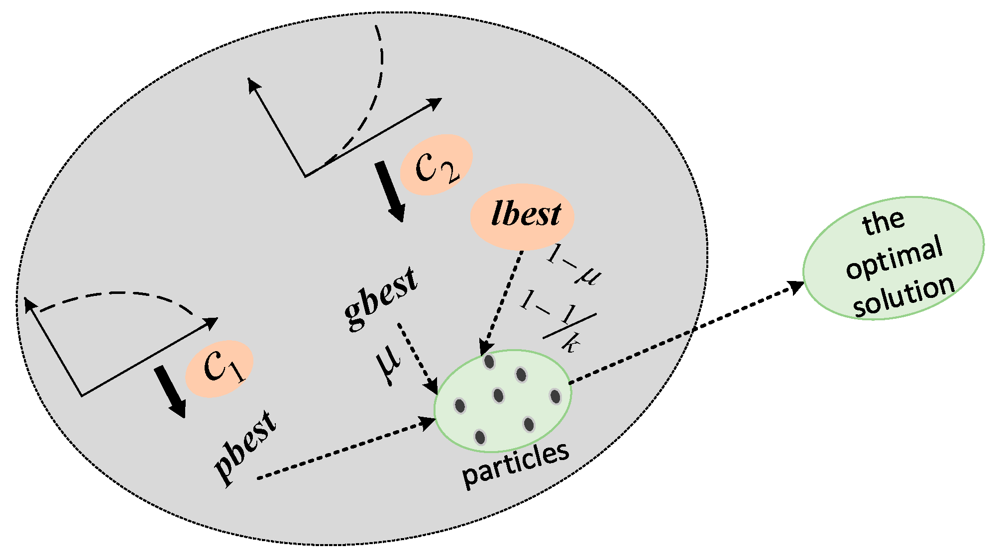
In brief, by introducing the time-varying learning factors and local best information, the improved PSO may ensure good exploration and exploitation capabilities even at the later stage of the optimization process. Figure 4 shows the schematic optimization process of our improved PSO.

3.2. Improved PSO-RBFNN

This section describes the improved PSO-RBFNN that can tune network parameters during the training process for higher accuracy. The RBFNN parameters optimization problem can be described as follows:

$$\begin{array}{l}find{\mathit{z}}_{op}=\arg \underset{\mathit{z}}{\max }g(\mathit{z})\\ s.t.\mathit{z}\in {\Re }^D\end{array}$$

(11)

where $\mathit{z}=({\sigma }_1,\dots ,{\sigma }_N,w_{11},\dots ,w_{mN},{\xi }_1,\dots ,{\xi }_m)$ is the position of a particle, with ${\sigma }_i$, $w_{ji}$, and ${\xi }_j$ being the width, connection weights, and residual sequence, respectively. The dimension of a particle, D, is determined by

$$D=N\times m+N+m$$

(12)

In the improved PSO-RBFNN, the fitness value of each particle represents the accuracy of the network. The fitness value is given by

$$g(\mathit{z})=\frac{1}{1+MSE({\mathit{y}}_r(\mathit{z}),{\mathit{y}}_e(\mathit{z}))}$$

(13)

where g(z) is the scalar fitness function; y_r(z) and y_e(z) are the network real output and expected output, respectively; MSE is the mean square error function referring to [34]. A larger fitness value implies a smaller MSE value. Based on Equations (5) and (9), the improved PSO is used to find the optimal particle ${\mathit{z}}_{op}=({\sigma }_1^{\prime },\dots ,{\sigma }_N^{\prime },w_{11}^{\prime },\dots ,w_{mN}^{\prime },{\xi }_1^{\prime },\dots ,{\xi }_m^{\prime })$, and then determine the optimal RBFNN. Figure 5 shows the schematic optimization process for obtaining ${\mathit{z}}_{op}$, and Figure 6 summarizes the procedure for the improved PSO-RBFNN.

4. Fast Multi-Objective Antenna Optimization Framework Combining MOEAs and Improved PSO-RBFNN Surrogate Model

In this section, we use the improved PSO-RBFNN surrogate model discussed in the previous section, rather than conventionally time-consuming EM simulations, to evaluate the antenna performance. The constructed antenna surrogate model is a black box for mapping the relationship between the antenna structure parameters and performance indexes (e.g., reflection coefficients, gain, efficiency, etc.). At the same time, the antenna multi-objective optimization is carried out by MOEAs. The whole optimization framework can be summarized as follows:

• Predefine antenna geometry vector x and design space X;
• Obtain the sample set S by sampling randomly in the design space X and obtain the response set Y by calling for EM simulation software;
• Obtain the optimal RBFNN parameters ${\mathit{z}}_{op}$ using improved PSO based on S, Y;
• Construct the improved PSO-RBFNN model ${\mathit{R}}_s(\mathit{x})$;
• Optimize the population by MOEAs and ${\mathit{R}}_s(\mathit{x})$;
• Stop when the termination condition is satisfied; otherwise, turn to step 5.

The flowchart of the fast multi-objective antenna optimization framework based on the MOEAs and improved PSO-RBFNN surrogate model is shown in Figure 7.

5. Verification Case Study and Discussions

In this section, the predicted reflection coefficients of a planar monopole antenna obtained by the improved PSO-RBFNN model are given and compared with those obtained by other surrogate models. Then, a planar miniaturized multiband antenna design is presented to verify the proposed multi-objective antenna optimization framework. The experiments are running in an environment equipped with 64-bit operating systems, 8 GB RAM, and Intel(R) Core(TM) i5-4590 CPU.

5.1. The Improved PSO-RBFNN Antenna Surrogate Model

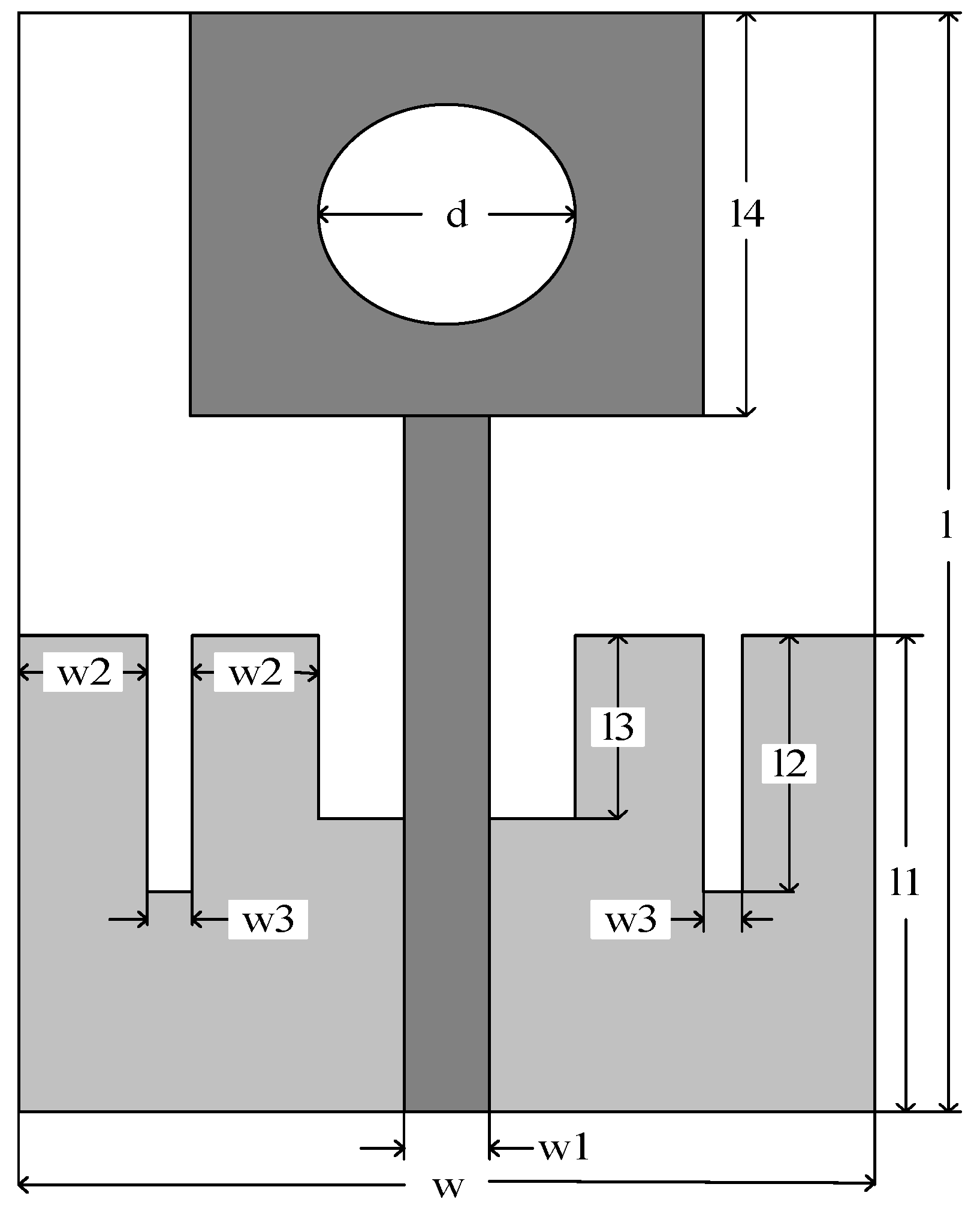
The initial geometry of planar miniaturized multiband antenna is shown in Figure 8 referring to Reference [6]. A rectangular microstrip patch with a circle slot is backed by a FR-4 substrate with a comb-shaped ground. The FR-4 substrate is of thickness 1.6 mm, permittivity 4.4, and loss tangent 0.02. Design parameters are $\mathit{x}={[dl{l}_1{l}_2{l}_3{l}_{4}w{w}_1{w}_2{w}_3]}^T$ and their initial ranges are given in

Table 1. Initial range of design parameters (units: mm).

Parameters	Range
d	[7, 10]
l	[26, 34]
l1	[11, 14]
l2	[8, 10]
l3	[6, 8]
l4	[10, 14]
w	[17, 23]
w1	[2, 4]
w2	[2, 4]
w3	[0.5, 1.5]

(all dimensions in mm).

When constructing an antenna surrogate model, 200 sample points are randomly initialized as the sample set S in a given design space X firstly. These sample points are transmitted to High Frequency Structure Simulator (HFSS) through HFSS-MATLAB-API to obtain the reflection coefficient response set Y. Then the first 180 sample points are used for model training and the remaining 20 are used for testing. The number of input layer neurons is 10, consistent with the number of antenna design parameters to be optimized, and the number of output layer neurons is 15, consistent with the number of frequency points at which reflection coefficients are computed. The number of hidden layer neurons is determined by comparing the errors of RBFNN with different numbers of hidden layer neurons. According to the experience of setting parameter in [35], the parameters of the improved PSO are set as follows: the population size M = 40; the maximum iteration number MaxIter = 1000; inertia weight $w=1$; nonlinear time-varying learning factors c₁, c₂ are adopted in (8) with c = 2 and α = 3 determined by the experimental tests; the adjusting factor μ = 0.5 is adopted in (9).

To demonstrate the superiority of the proposed improved PSO-RBFNN model over conventional PSO-RBFNN [24], Figure 9 shows the fitness curve of these two models in the training process. It can be observed that the fitness values of our proposed model are significantly larger than the conventional one, indicating that our model can achieve a much lower training error MSE. Furthermore, Figure 10 compares the scatter plots of the predicted S11 results by Kriging [5], RBFNN [11], PSO-RBFNN [24] and improved PSO-RBFNN relative to the simulations obtained by HFSS. It is clearly observed that the testing points in Figure 10a are more concentrated on the diagonal compared with Figure 10b–d, demonstrating that the proposed model has better prediction ability than Kriging, RBF, and conventional PSO-RBFNN using the same sample points. Besides, the time cost of different surrogate models and HFSS simulations are tabulated in

Table 2. Time cost of different surrogate models and HFSS simulations (units: s).

Methods	HFSS	Kriging [5]	RBFNN [11]	PSO-RBFNN [24]	Improved PSO-RBFNN
Total time	1017.820	0.413	0.165	0.043	0.039
Average time	50.891	0.021	0.008	0.002	0.002

. The results indicate that the use of various surrogate models greatly reduces the computational time compared to HFSS simulation.

In summary, our proposed PSO-RBFNN model can be used for performance prediction efficiently instead of EM simulation software and achieve a fast multi-objective optimization with the help of MOEAs for a predefined antenna geometry.

5.2. Pareto-Optimal Designs of Planar Miniaturized Multiband Antenna

The fast multi-objective optimization of the planar antenna geometry given in Figure 8 is implemented using MOEA/D [36] and the improved PSO-RBFNN model. Two design goals are to be achieved: (i) the reflection coefficients are lower than −10dB within three frequency bands of 2.40~2.60 GHz, 3.30~3.80 GHz, 5.00~5.85 GHz, covering the entire WLAN2.4/5.2/5.8 GHz and WiMAX3.5 GHz bands (objective F₁); and (ii) the size of antenna structure is reduced to satisfy the need of antenna miniaturization in portable devices (objective F₂). The objective function of F₁ is specified as

$$F_1=\frac{1}{N}{\displaystyle \sum _{i=1}^{n}Q(f_i)}$$

(14)

$$Q(f_i)=\{\begin{array}{ll}\left|S_{11}(f_i)\right|& \left|S_{11}(f_i)\right|>-10\\ -10& \left|S_{11}(f_i)\right|\le -10\end{array}$$

(15)

where f_i is the ith sample within the given operation bands; $S_{11}(f_i)$ is the reflection coefficient at f_i; N is the total number of sampling frequencies. The objective function of F₂ is defined as

$$F_2=w\times l$$

(16)

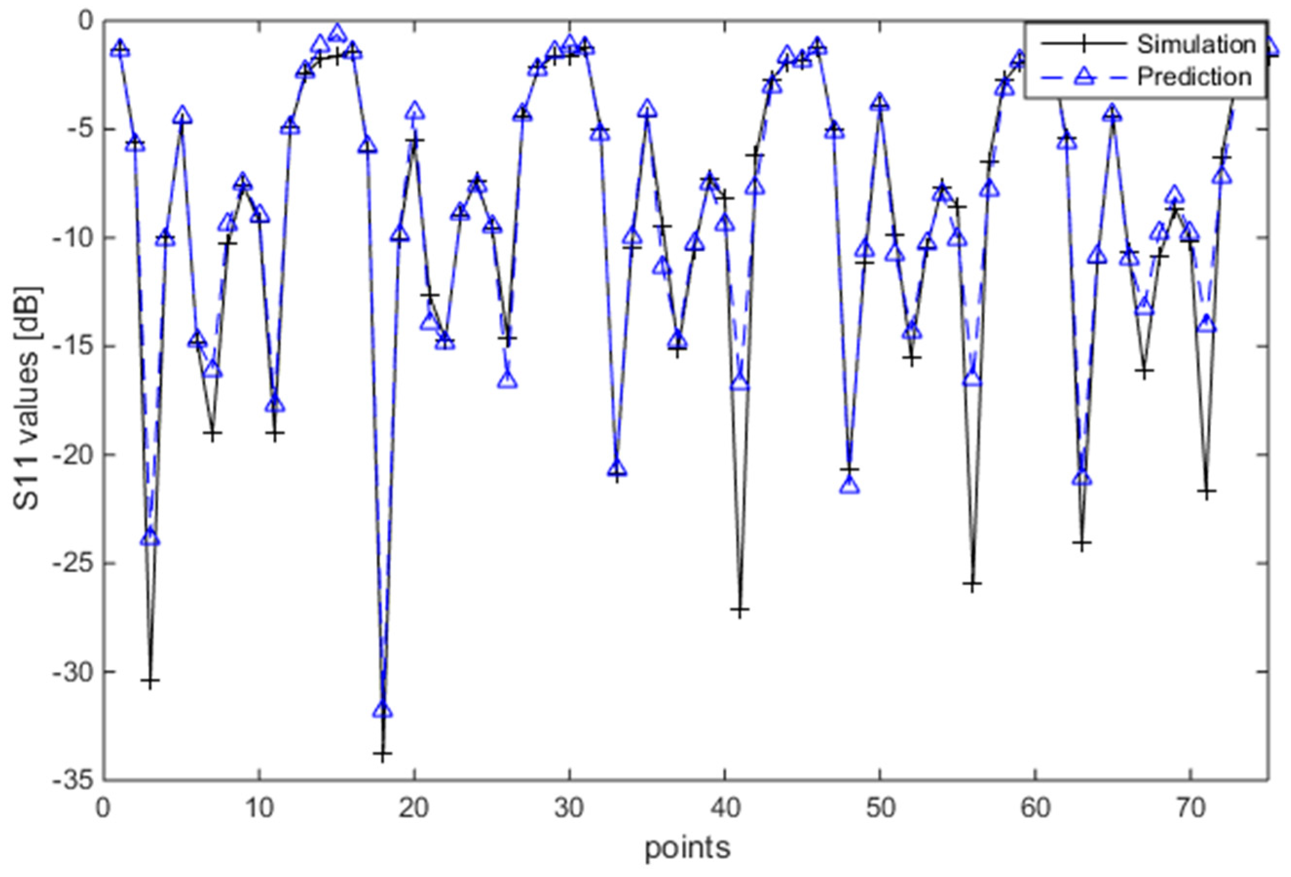
According to the principles of setting parameters for MOEA/D in Reference [36], the number of population is chosen as 100, and the maximum number of iterations is chosen as 150. The representations of the Pareto set during the optimization process for the planar miniaturized multiband antenna is given in Figure 11, which displays the evolution behavior of the objective functions.

Table 3. Miniaturized multiband planar antenna: selected Pareto-optimal designs.

Designs	${\mathit{x}}^{(1)}$	${\mathit{x}}^{(2)}$	${\mathit{x}}^{(3)}$	${\mathit{x}}^{(4)}$	${\mathit{x}}^{(5)}$
$F_1[dB]$	−16.02	−15.67	−15.45	−15.03	−14.71
$F_2[m{m}^2]$	634.92	628.00	617.97	602.76	577.17
d	8.58	8.61	8.76	8.69	8.27
l	31.20	31.40	29.26	29.26	28.90
l1	12.70	12.50	12.00	11.95	11.09
l2	8.80	8.80	9.04	9.04	8.79
l3	6.92	6.90	7.28	7.21	7.01
l4	11.43	11.43	11.73	11.73	11.37
w	20.35	20.00	21.12	20.60	19.97
w1	3.23	3.23	3.34	3.31	3.13
w2	3.10	3.10	3.27	3.27	3.27
w3	1.01	1.00	1.19	1.17	1.01

shows the detailed antenna parameters on the final selected designs. It can be seen from Figure 11 and Table 3 that achievements of the two design objectives are actually in conflict. To show the fitting ability of the PSO-RBFNN model, the HFSS simulated and predicted S₁₁ for the Pareto-optimal designs are given in Figure 12. It can be observed that the predicted S₁₁ well match the simulated S₁₁.

To validate the feasibility of the proposed model, the predicted results of fitness F₁ and percentage error relative to the HFSS simulations are given in Figure 13.

Furthermore, the proposed PSO-RBFNN model is compared with other competitive techniques in terms of the computation time. Method 1 is direct MOEA/D-based optimization combined with HFSS simulation, and Method 2 is MOEA/D with RBF model [11]. The detailed computational cost is shown in

Table 4. Comparison of computational cost among different antenna optimization methods.

Optimization Method	Number of EM Simulations	CPU Time/h
		Total	Relative
Method 1	15,100	213.51	100%
Method 2	200	2.93	1.37%
This work	200	2.98	1.40%

. One EM simulation takes about 51 s under the high-fidelity running environment. This work and Method 2 use only 1.37% and 1.40% of the computational time of Method 1, 2.93 h and 2.98 h, respectively. This work takes a bit longer time than Method 2 due to the PSO optimization of RBF network parameters, however, it is still more computationally efficient than Method 1 with 213.51 h. In conclusion, the proposed PSO-RBFNN method enables realization of antenna design solutions satisfying multiple requirements within affordable computational cost. This method significantly reduces the design cycles of multi-parameter multi-objective antenna optimizations.

6. Conclusions

An improved PSO-RBFNN antenna surrogate model is developed and applied to the fast multi-objective design of multi-parameter antenna structures. To overcome the limitations of conventional RBFNN, an improved PSO algorithm is proposed to determine the optimal RBF network parameters. This improved PSO can balance the ability of exploration and exploitation of particles in the search space by designing time-varying learning factors. Moreover, it can increase the diversity of swarms to obtain an optimal solution by introducing the local best information, thus avoiding premature convergence. By integrating the improved PSO-RBFNN surrogate model with MOEAs, a fast multi-objective antenna optimization framework is then established. A planar miniaturized multiband antenna design is presented, demonstrating that our proposed method is more competitive with considerable computational savings and good design efficiency compared to the previously published methods.

References

- Choi, K.; Jang, D.H.; Kang, S.I.; Lee, J.H.; Chung, T.K.; Kim, H.S. Hybrid algorithm combing genetic algorithm with evolution strategy for antenna design. IEEE Trans. Magn. 2016, 52. [Google Scholar] [CrossRef]
- Dong, J.; Li, Q.; Deng, L. Design of fragment-type antenna structure using an improved BPSO. IEEE Trans. Antennas Propag. 2018, 66, 564–571. [Google Scholar] [CrossRef]
- Carvalho, R.; Saldanha, R.R.; Gomes, B.N.; Lisboa, A.C.; Martins, A.X. A multi-objective evolutionary algorithm based on decomposition for optimal design of Yagi-Uda antennas. IEEE Trans. Magn. 2012, 48, 803–806. [Google Scholar] [CrossRef]
- Noras, J.M.; Abd-Alhameed, R.A.; Abdulraheem, Y.I.; Abdullah, A.S.; Mohammed, H.J.; Ali, R.S. Design of a uniplanar printed triple band-rejected ultra-wideband antenna using particle swarm optimisation and the firefly algorithm. IET Microw. Antennas Propag. 2016, 10, 31–37. [Google Scholar]
- Koziel, S.; Ogurtsov, S. Multi-objective design of antennas using variable-fidelity simulations and surrogate models. IEEE Trans. Antennas Propag. 2013, 61, 5931–5939. [Google Scholar] [CrossRef]
- Dong, J.; Li, Q.; Deng, L. Fast multi-objective optimization of multi-parameter antenna structures based on improved MOEA/D with surrogate-assisted model. AEU-Int. J. Electron. Commun. 2017, 72, 192–199. [Google Scholar] [CrossRef] [Green Version]
- Liu, B.; Aliakbarian, H.; Ma, Z.; Vandenbosch, G.A.; Gielen, G.; Excell, P. An Efficient method for antenna design optimization based on evolutionary computation and machine learning techniques. IEEE Trans. Antennas Propag. 2014, 62, 7–18. [Google Scholar] [CrossRef]
- Jacobs, J.P. Efficient Resonant Frequency Modeling for Dual-Band Microstrip Antennas by Gaussian Process Regression. IEEE Antennas Wirel. Propag. Lett. 2015, 14, 337–341. [Google Scholar] [CrossRef]
- Qin, W.; Dong, J.; Wang, M.; Li, Y.; Wang, S. Fast Antenna Design Using Multi-Objective Evolutionary Algorithms and Artificial Neural Networks. In Proceedings of the 12th International Symposium on Antennas, Propagation and EM Theory (ISAPE), Hangzhou, China, 3–6 December 2018. [Google Scholar]
- Dong, J.; Qin, W.; Wang, M. Fast Multi-Objective Optimization of Multi-Parameter Antenna Structures Based on Improved BPNN Surrogate Model. IEEE Access 2019, 7, 77692–77701. [Google Scholar] [CrossRef]
- Mohamed, M.D.A.; Soliman, E.A.; El-Gamal, M.A. Optimization and characterization of electromagnetically coupled patch antennas using RBF neural networks. J. Electromagn. Waves Appl. 2006, 20, 1101–1114. [Google Scholar] [CrossRef]
- Mishra, S.; Yadav, R.N.; Singh, R.P. Directivity estimations for short dipole antenna arrays using radial basis function neural networks. IEEE Antennas Wirel. Propag. Lett. 2015, 14, 1219–1222. [Google Scholar] [CrossRef]
- Jones, D.L. A taxonomy of global optimization methods based on response surfaces. J. Glob. Optim. 2001, 21, 345–383. [Google Scholar] [CrossRef]
- Santner, T.J.; Williams, B.J.; Notz, W.I. The Design and Analysis of Computer Experiments; Springer: New York, NY, USA, 2003. [Google Scholar]
- Thakare, V.V.; Singhal, P.K. Bandwidth Analysis by Introducing Slots in Microstrip Antenna Design Using ANN. Prog. Electromagn. Res. M 2009, 9, 107–122. [Google Scholar] [CrossRef]
- Chen, D. Research on traffic flow prediction in the big data environment based on the improved RBF neural network. IEEE Trans. Ind. Inform. 2017, 13, 2000–2008. [Google Scholar] [CrossRef]
- Li, M.M.; Verma, B. Nonlinear curve fitting to stopping power data using RBF neural networks. Expert Syst. Appl. 2016, 45, 161–171. [Google Scholar] [CrossRef]
- Huang, S.C.; Do, B.H. Radial Basis Function Based Neural Network for Motion Detection in Dynamic Scenes. IEEE Trans. Cybern. 2013, 44, 114–125. [Google Scholar] [CrossRef] [PubMed]
- Zhang, Y.; Zhou, Q.; Sun, C.; Lei, S.; Liu, Y.; Song, Y. RBF Neural Network and ANFIS-Based Short-Term Load Forecasting Approach in Real-Time Price Environment. IEEE Trans. Power Syst. 2008, 23, 853–858. [Google Scholar] [CrossRef]
- Park, J.; Sandberg, I.W. Universal approximation using radial-basis-function networks. Neural Comput. 1991, 3, 246–257. [Google Scholar] [CrossRef]
- Zhang, R.; Xu, Z.B.; Huang, G.B.; Wang, D.H. Global convergence of online BP training with dynamic learning rate. IEEE Trans. Neural Netw. Learn. Syst. 2012, 23, 330–341. [Google Scholar] [CrossRef]
- Xu, Z.B.; Zhang, R.; Jing, W.F. When does online bp training converge? IEEE Trans. Neural Netw. 2009, 20, 1529–1539. [Google Scholar]
- Feng, H.M. Self-generation RBFNs using evolutional PSO learning. Neurocomputing 2006, 70, 241–251. [Google Scholar] [CrossRef]
- Fei, X.; Sun, Y.; Ruan, X. A simulation analysis method based on PSO-RBF model and its application. Clust. Comput. 2018, 1–7. [Google Scholar] [CrossRef]
- Gutierrez, P.A.; Hervas-Martinez, C.; Martinez-Estudillo, F.J. Logistic regression by means of evolutionary radial basis function neural networks. IEEE Trans. Neural Netw. 2011, 22, 246–263. [Google Scholar] [CrossRef] [PubMed]
- Lee, C.M.; Ko, C.N. Time series prediction using rbf neural networks with a nonlinear time-varying evolution pso algorithm. Neurocomputing 2009, 73, 449–460. [Google Scholar] [CrossRef]
- Koziel, S.; Bekasiwewicz, A. Fast multi-objective surrogate-assisted design of multi-parameter antenna structures through rotational design space reduction. IET Microw. Antennas Propag. 2016, 10, 624–630. [Google Scholar] [CrossRef]
- Moody, J.; Darken, C.J. Fast learning in networks of locally-tuned processing units. Neural Comput. 1989, 1, 281–294. [Google Scholar] [CrossRef]
- Zhang, L.; Li, K.; He, H.; Irwin, G.W. A new discrete-continuous algorithm for radial basis function networks construction. IEEE Trans. Neural Netw. Learn. Syst. 2013, 24, 1785–1798. [Google Scholar] [CrossRef] [PubMed]
- Chen, L.L.; Liao, C.; Lin, W.; Chang, L.; Zhong, X.M. Hybrid-Surrogate-Model-Based Efficient Global Optimization for High-Dimensional Antenna Design. Prog. Electromagn. Res. 2012, 124, 85–100. [Google Scholar] [CrossRef]
- Kennedy, J.; Eberhart, R.C. Particle swarm optimization. In Proceedings of the 1995 IEEE International Conference on Neural Networks, Perth, Australia, 27 November–1 December 1995; pp. 1942–1948. [Google Scholar]
- Lynn, N.; Suganthan, P.N. Heterogeneous comprehensive learning particle swarm optimization with enhanced exploration and exploitation. Swarm Evol. Comput. 2015, 24, 11–24. [Google Scholar] [CrossRef]
- Islam, M.J.; Li, X.; Mei, Y. A Time-Varying Transfer Function for Balancing the Exploration and Exploitation ability of a Binary PSO. Appl. Soft Comput. 2017, 59, 182–196. [Google Scholar] [CrossRef]
- Zhang, Y.; Chen, Q. Prediction of building energy consumption based on PSO-RBF neural network. In Proceedings of the 2014 IEEE International Conference on System Science and Engineering (ICSSE), Shanghai, China, 11–13 July 2014; pp. 60–63. [Google Scholar]
- Jin, N.; Rahmat-Samii, Y. Advances in particle swarm optimization for antenna designs: Real-number, binary, single-objective and multiobjective implementations. IEEE Trans. Antennas Propag. 2007, 55, 556–567. [Google Scholar] [CrossRef]
- Zhang, Q.; Li, H. MOEA/D: A multiobjective evolutionary algorithm based on decomposition. IEEE Trans. Evol. Comput. 2007, 11, 712–731. [Google Scholar] [CrossRef]
Figure 1.
Pareto front (PF) of two goals.
Figure 2.
Structure of a multiple-input multiple-output radial basis function neural network (RBFNN).
Figure 3.
Curves of time-varying learning factors: (a) with different values of α when c = 2; (b) with different values of c when α = 3.
Figure 4.
Schematic Optimization process of our improved particle swarm optimization (PSO).
Figure 5.
The schematic optimization process for obtaining .