Optimal Strategy to Select Load Identification Features by Using a Particle Resampling Algorithm

1
Electric Power Research Institute, CSG, Guangzhou 510663, China
2
Department of Artificial Intelligence and Automation, Wuhan University, Wuhan 430072, China
*
Author to whom correspondence should be addressed.
Appl. Sci. 2019, 9(13), 2622; https://doi.org/10.3390/app9132622
Submission received: 20 May 2019
/
Revised: 12 June 2019
/
Accepted: 26 June 2019
/
Published: 28 June 2019
(This article belongs to the Special Issue Sustainable Energy Systems Planning, Integration and Management)
Abstract
:This paper proposes a robust strategy to select the load identification features, which is based on particle resampling to promote the performance for the successive load identification. Firstly, the sliding window incorporated with the bilateral cumulative sum control chart (CUSUM) method is utilized to obtain the load event. Then, the minimum inner-class variance, using the time-serial data, is introduced to judge the happened time as precise as possible, thus marking the changing point of the state of load for the following feature extraction. Due to the fluctuating data of current and voltage sampled by the monitoring device, the particle resampling method, containing the importance principle, is applied to find the steady and effectiveness point, ensuring that the obtained features have the desired fit with its actual features. The fitness measurement is then carried out by using the 2-D fuzzy theory. Finally, the proposed method was tested on the real household measurements in the labs. The result demonstrates an improvement in obtaining the desired load features when applied to the real household for the following load identification.
1. Introduction
Recently, non-intrusive load monitoring (NILM) has gained major attention in the research field of smart grid [1], which aims to separate household energy consumption data collected from a single point of measurement into appliance-level consumption data. Since this technology was invented by George W. Hart et al. [2] in the early 1980s, non-intrusive load monitoring has been considered as a low-cost alternative to attaching individual monitors on each appliance, in contrast to the intrusive load monitoring method. In addition, it can provide information, such as energy usage, the state of the device, and so on. Up to now, the technology of NILM is becoming the state-of-the-art in the field of smart grid, which is built on signal processing, pattern recognition, and such deep learning algorithms for recognizing the power consumed in a household.
In general, the existing NILM methods can be divided into two main categories: event-based and non-event based [3]. The event-based approaches attempt to detect the changes of the state according to the significant change in power and then the features are obtained according to the changes in states. The recognition of appliances is then carried out by using a method, like the matching method and the clustering method, which is modeled by the real appliance recorded in the database. Non-event based NILM approaches are related to the machine learning from the big data collected by the single appliance or mixture of appliances during their working. However, the fundamental principle of load identification is dependent on the extraction of a stable and reliable load feature.
Load feature, also named load signature, is often represented during the appliance’s work, including the start, running, and the stop state. Generally speaking, the feature of the start state and the stop state is the most remarkable during the extraction of the load feature. In the literature, the feature extraction stage can judge the algorithm type of the appliance, such as the transient state features-based algorithms and the steady state features-based algorithms [4,5,6]. Chang and Lian [7] adopted the wavelet transform coefficients (WTCs) to get the turn-on/off transient signal identification of load events. Similarly, a multi-resolution S-transform-based transient feature extraction scheme was proposed and presented in [8]. However, transient state features were obtained only if the sampling frequency exceeded 1000 Hz [9]. Taking into account the implementation, the steady state features-based algorithms seem to be more economical than the transient state features-based algorithms. Dinesh and Perera proposed a feature extraction method in [10] by using a modified mean shift algorithm at a low sampling rate. In [11], Leen’s team shared a modified version of the chi-square goodness-of-fit test for event detection and getting the load features. Moreover, there are also many other methods based on stable load characteristics [12].
Those works above, however, almost all focused on the local information of the load during its turning on or off. The features extracted by the existing methods might not reach satisfactory predictive performance for load identification. Hence, in this paper, a particle resampling algorithm is proposed to select the desired load identification features, and then using the fuzzy theory, the method is tested with real data. The results showed that the proposed method that employed the steady state of load signatures, such as active power and reactive power, can identify the load accurately during load disaggregation.
2. Materials and Methods
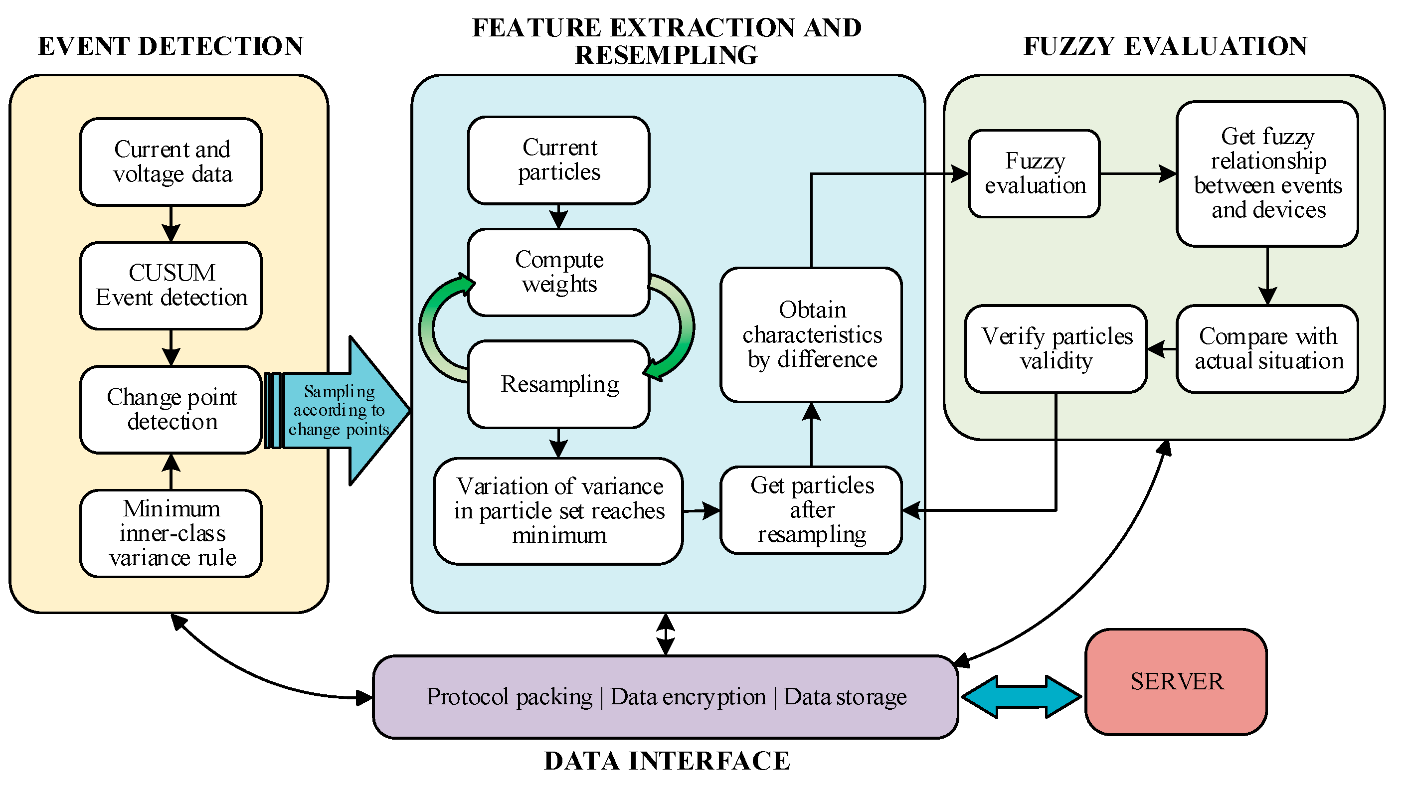
This section mainly describes the materials and methods used for selecting the desired features and their evaluation. Generally speaking, the load identification method structure mainly consisted of the following three parts: (1) event detection, (2) feature extraction, and (3) fuzzy evaluation and identification. In this work, we mainly focused on feature extraction, and the whole framework is illustrated in Figure 1. In the event detection, the bilateral cumulative cum control chart (CUSUM) algorithm, combined with minimum inner-class variance rule method, was used to ensure that the load events and the change points were detected accurately. According to these change points, the resampling method was introduced to avoid the influence by the fluctuations of the voltage and current. Besides, the extracted features were validated by using the fuzzy evaluation, and, thus, can be applied to load identification. And then, the work is described as follows.
2.1. Event Detection Algorithm
Load event, which is defined as changes in load characteristics caused by switching on/off or state changes of individual devices [13], is the first and significant step in the load identification. In practical applications, the reliability and accuracy of event detection could be affected by the unpredicted switching and the interference of voltage and current fluctuations. In this paper, a non-parametric cumulative sum control chart (CUSUM) event detection algorithm was used for load detection. This method accumulates the sample data as well as the small deviation of the process. Since the accumulated value is significantly higher, a load event occurs. In addition, the method can be extended to the algorithm bilateral CUSUM due to the fact that the load events about turning on and turning off usually happened in pairs.
Let the time series of extracting load data be X = {x (k)}, k = 1, 2, … The statistic function in nonparametric bilateral CUSUM algorithm is defined as:
where μ0 is the average value before the occurrence of the load event, θ is random noise introduced from outside, and fk+ and fk− are the random variable with 0 being the mean (i.e., random fluctuations around zero). When the load is turning on, xk will increase and fk+ will have an increasing trend. On the contrary, the load when turned off will make fk− decrease. So the load event can be detected when the change exceeds the threshold h. Usually, the threshold h is set according to the lowest power value of the load.
To make the Equation (1) more understandable, Figure 2 gives a detailed description of the CUSUM. The load is a continuous change on the time axis, i.e., the mean μ0 in the Equation (1) is changed with time. The sliding window model was then constructed to constrain the accumulated sum to ensure the load event was acquired accurately. So the W1 window and W2 window were modeled in this paper. The W1 window was used to calculate the mean value μ0 of the sampling sequence. The W2 window was considered as the basis for judging whether a load event has occurred. From Equation (1), the value of fk+ in window W2 gradually accumulates when the value of xi increases. So when fk+ exceeds a certain threshold h, the load occurs. On the contrary, the value of fk+ in window W2 fluctuates within a small range if no load event is detected. In this case, the W1 and W2 windows slide to the new sampling point and continue to detect.
Considering that the threshold h is a global parameter, it is usually determined by the minimum load characteristic value. Therefore, to reduce the influence of the manually set threshold h, the minimum inner-class variance rule can be taken as the change point detection method. In the load event detection window, the active power data samples are classified into two categories: class C0 {x1, x2, …, xk} and class C1 {xk+1, xk+2, …, xV}, where V is the sample length in the window, let:
When the objective function
reaches the minimum and |m(C1) − m(C0)| is greater than the set active power change value, the time of the change point could be found.
2.2. Identification Feature Extraction and Resampling
Since the change point was found by the above method, the feature of the load could be obtained by using the load characteristics of the changes [14]. Usually, the load event is determined based on physical changes in current, voltage, and other power information. Therefore, the load characteristics of these changes can be considered as the characteristics of the switching of the electrical device. For example, Figure 3 illustrates three types of load, named resistive load, capacitive load, and inductive load, which have different current phases for their capacitive reactance and opposite impedance performances. We can figure out the active power P by the voltage U, current I, and their phase difference φ that:
P = UIcosφ.
Similarly, the reactive power Q can be described as:
Q = UIsinφ.
Active power and reactive power can be calculated by Equations (5) and (6), and they can distinguish between the different types of loads according to their values. Moreover, active power and reactive power can be captured by low-frequency meters. In this paper, active power P and reactive power Q were adopted as the features.
In order to clearly illustrate the extraction of the load features, including the active and reactive characteristics, let P(t) denote the active power variation with time t for an example. Usually, it is statistically stable. However, once the load changes the status, the P(t) may undergo large changes at that time. So, the difference of P can represent the change of the status of the device, thus the value of P(t) can be disaggregated. Here, we denote the ΔP = P(t + Δt) − P(t) as the difference of P, and the P(t) satisfies the condition as follows:
where P(t) is the active power at time t; m is the total number of load in the database; ai is the mark of the state of load, where ai = 1 indicates the running state and ai = 0 means turned off; and T is the time interval.
Similarly, the reactive characteristic (or called the difference of Q) ΔQ = Q(t + Δt) − Q(t) at time t satisfies the condition as follows:
From Equations (7) and (8), it can be observed that the extraction of load characteristics from power load switching is related to the time of change point, i.e., the time interval T.
Although the change point is found according to the rules of the minimum inner-class variance, the voltage and current fluctuations make it difficult to determine this time interval T. Usually, the different time T can obtain the different P and Q features. In some papers [15,16,17], the time T is selected as the point after the change point. For some situations, the changes in P and Q may mismatch the load during load identification. So, in this paper, the importance resampling method was proposed to avoid the uncertainty of time interval T and the influence of power load information fluctuation.
The resampling algorithm is often used to solve the sequential importance sampling algorithm [18]. At present, there are many kinds of resampling algorithms [19,20]. In this paper, the importance resampling algorithm is adopted.
To further explain, Figure 4 describes the process of resampling. It can be seen that this method regards the characteristics at each time as a particle and resamples the importance of each particle according to the distribution of particles before and after the change point. The specific process is as follows:
Step 0: Assuming that the load is put into operation, the change point time t is obtained. Let k = 0, which randomly gets N particles after the current time t and before the next change point, and initializes each particle xi with equal weight , i = 1, …, N.
Step 1: Importance sampling is used to distribute the weight of each particle. For each particle i = 1, …, N, estimate the weight of importance ωk according to the degree of center deviation:
where Ω is the particle set. And we normalize Ω to get new weight .
Step 2: We discard those particles with smaller weights and substitute sampling near the particles with larger weights.
Step 3: Set and repeat the process of Step 1 and Step 2 to minimize the variation of variance in particle set Ω.
Step 4: We differentiate the current load characteristics in the particle set from the previously recorded load characteristics to extract the load variation characteristics.
2.3. Fuzzy Evaluation Method
It is necessary to propose an evaluation method based on fuzzy membership after the identification features obtained by using the resampling method. The concept of the fuzzy set was first introduced in [21]. Fuzzy theory is a kind of transaction that copes with the concept of uncertainty through membership degree [22]. So, it can evaluate the relationship between load identification features and real load characteristics in the database. Considering the use of P and Q features as identification features, the 2-dimension fuzzy set are used in this paper.
Suppose that there are n loads, A1, A2, A3, …, An, with two evaluation factors, active power (f1) and reactive power (f2). Consider m linguistic hedges Ψ. Note that it is possible to consider an objective application between the finite chain L and the ordinal scale Ψ, which keeps the order. Thus, each normal convex fuzzy subset defined on the ordinal scale Ψ can be considered as a discrete fuzzy number with the support L, L = {1, 2, …, m}. Then the following data can be set for the load Ai (i = 1, 2, …, n):
where Ai1 and Ai2 are two discrete fuzzy numbers of the metric feature, m is the evaluation coefficient level, and xijk is the evaluation factor of the object Ai (i = 1, 2, …, n).
Then, the mean value can be worked out as . Let elements in K be the number (or numbers) that is (or are) closest to the mean value μ(Aij) in L = {1, 2, …, m}, i.e., . It is obvious that the number of the elements of K can only be one or two. Then the following method can be given to construct one-dimensional discrete fuzzy number : R → [0, 1] for any i = 1, 2, …, n and any j = 1, 2.
As K only has one element (denoted by k0), can be defined as:
As K has two elements (denoted by k0 and k0 + 1), can be defined as:
where , , , , and i = 1, 2, …, n, j = 1, 2. We stipulate that as , as , and as in Equations (10) and (11).
Then, we can construct the two-dimensional unite discrete fuzzy number of and to express device Ai according to for any X = (x1, x2) ∈ R2 (i = 1, 2, …, n). Next, the centroid can be calculated based on the resulting matrix:
In order to obtain the final evaluation value, it is necessary to combine the ratios of the two criteria of the centroid p = (p1, p2), where p1 and p2 describe the importance of the features of the centroid counterpart. Considering that the combination of the centroid and weight is more conducive to the comprehensive evaluation of the possibility of the category, the metric can be established as follows:
Finally, through comparing the v values of different objects, the actual object, which has the highest evaluation value, is found. Therefore, if the obtained load identification features had the largest evaluation value, the actual object was determined.
3. Experiments and Results
This section describes the experimental procedure and discusses the obtained results for demonstrating the efficiency of our method. Electrical characteristics, such as current and voltage, of the home were obtained through the monitoring device that was installed at the power inlet of the experimental resident user.
3.1. Laboratory Validation
The experiments used five devices, including a rice cooker, microwave oven, induction cooker, air conditioner, and kettle. Firstly, the individual device underwent the state of turning on and turning off several times, as seen in Figure 5 for an example. Then, the active power and reactive power were obtained through data statistical analysis, as shown in Table 1. Finally, these load features were recorded in the MySQL database. Meanwhile, the threshold was h = 350, the minimum change load active power was 100 watts, and the event detection window length was 20 sample points for the load event detection in this example.
Figure 6 shows the above load during its state of turning on and/or turning off in the actual test. The order sequence is air conditioner on, induction cooker on, kettle on, microwave oven on, rice cooker on, then kettle off, induction cooker off, microwave oven off, rice cooker off, and air conditioner off, respectively, as shown in Table 2. Table 3 shows the timing of the change point obtained by the original CUSUM load event detection [23]. It can be seen that there was a certain multi-detection phenomenon due to the increase slowly of active power after turning on the air conditioner. Nevertheless, our method could detect this type of load and could get better result accuracy, as shown in Table 4. So the resulting change points is approximated by the real-time change points.
Further, Table 4 shows the difference of P and Q in the case of the time interval T = 1, using the change point detected by our method. It was found that the obtained load identification features had a certain distance from the corresponding actual load characteristic information shown in Table 1. In particular, the active power with slow increases, such as the air conditioner, greatly differed from the actual characteristic values, which may fail to identify the load. In addition, these loads have different load characteristics between on and off, such as electric kettles and induction cookers. In this paper, the particle resampling algorithm was used to extract features. By retaining the particles with larger weights, some off-center particles were discarded and the best load characteristics could then be found.
Taking the air conditioning load switching on and off as an example, Figure 7 shows the whole process of particle resampling. It can be seen that, in Figure 7a,b, there are a few particles far away from the center point obtained by the whole particles and that the distribution is not uniform. So, these particles can be replaced by the resampling method, as seen in Figure 7c,d. These particles almost converge to a state after resampling. In order to describe the state clearly, Table 5 illustrates the fluctuation range of active power and reactive power. After resampling, the fluctuation range is lower than before resampling. So, the load feature can be obtained properly. Here, we used the difference of the center of resampling particles after the device was switched on and the center of the resampling particles before the device was switched on as the load feature. Finally, the obtained active power was 462.17 W and the reactive power was −150.55 Var. Referring to Table 1, it can be found that the value of the obtained active power and reactive power was in the range of air conditioning, rather than the range of other devices. So we can easily identify this device.
In addition, Table 6 shows the obtained P and Q features using our method. It can be seen that the value of P and Q had a better correlation with the load features in Table 1. Notably, the obtained value did not change the sign if the status of the load was turning off.
In order to verify the effectiveness of the above-obtained features, here, an induction cooker, a kettle, an air conditioner, a rice cooker, and a microwave oven are represented by A1, A2, A3, A4, and A5. In addition, nine levels of fuzzy language are used for active and reactive features:
respectively, denoted as extremely bad, very bad, bad, more or less bad, fair, more or less good, good, very good, and extremely good, and they are linked to the finite chain L = {1, 2, …, 9}. According to the previous two-dimensional fuzzy membership evaluation method, the results of the final evaluation are shown in Table 7. It is not difficult to see that the load characteristics obtained after the load event detection could basically match the actual switched electrical equipment.
3.2. Validated on REDD
The reference energy disaggregation dataset (REDD) is a freely available data presented by J. Z. Kolter and M. Johnson [24]. The REDD contains detailed power usage information from several homes, which provides circuit-level data, rather than plug-level data. Here, we used it for demonstrating the performance of the event detection and feature extraction.
3.2.1. Event Detection
This part presents the performance of the proposed bilateral CUSUM event detection method and makes a comparison with the original CUSUM method over the REDD. In this work, the confusion matrix-based metrics are taken as the evaluation metric [25]. So, the detection events were divided into four categories: true positive (TP), true negative (TN), false positive (PF), and false negative (FN). Only TP, FP, and FN are considered in event detection performance evaluation because TN is usually infinite. On the basis of the confusion matrix, the evaluation can be carried out by using the following measurements, as seen in Table 8.
Taking data from House3 in the REDD as an example, Table 9 illustrates the main metrics using the bilateral CUSUM, original CUSUM, and BIC (Bayesian information criterion) detector [27]. This is a day-of-event detection statistics. From the results, it can be seen that the bilateral CUSUM had the highest Score. The original CUSUM event detection method had the highest true positive rate (TPR), but it often had multiple FPs. The BIC detector had the lowest TPR and Score. By comparison, the bilateral CUSUM method performed better than the other two methods.
3.2.2. Feature Extraction on REDD
The data in the REDD in House 3 contained 10 appliances: lighting2/4/5, refrigerator, furnace, washer1/2, microwave, bathroom_gfi, and kitchen outlets2. The characteristics of a single electrical equipment were obtained from the statistics of the information from a single channel. This paper mainly focuses on active and reactive power information. In order to demonstrate the effectiveness of the feature extraction method, the resampling and average value method [27] were compared. Figure 8 and Figure 9 illustrate the two-dimensional discrete fuzzy number. It can be seen that the particles obtained by the resampling method had higher overall accuracy in hypothesis and identification. Although the particles selected by the average value method and resampling method had a good performance on furnace, washer1, lighting4, and lighting5, the particles selected by the average value method made mistakes in identifying bathroom_gfi and kitchen_outlets2 as these devices having similar features. This demonstrates that our method has advantages in terms of feature extraction.
4. Conclusions and Future Works
In this paper, a load identification features selection method was proposed and validated by using the laboratory dataset and REDD. The experiment showed that our method has the ability to extract the desired features, which may accurately match the features of the device recorded in the database. In the experiment, the performance of load event detection was also carried out. A bilateral CUSUM combined with the minimum inner-class variance approach that we proposed also promoted the detection effectiveness, especially for the climbing character of a load event. Besides, the resampling method incorporated in our method was used to find the stable characteristics of the load event, thus obtaining the desired features. Through the 2-D fuzzy membership measurement, it was found that the feature extracted by the resampling method is closer to that of the actual device, and can be applied to load identification. However, this resampling method requires a relatively stable switching period of the device. In practice, the device being turned on or off is random, thus the obtained features may fail to match the features of devices in the database.
In the future, the limitations mentioned above should be carefully considered. For example, some devices have a short duration after state switching, and the corresponding steady-state time is also very short. In this case, the method combining the transient features may work better. Moreover, different algorithms, based on different features, may be valid for certain types of devices. Therefore, it is necessary and feasible to integrate the proposed method with other complementary NILM models.
Author Contributions
Methodology, H.H.; Validation, Y.X.; Formal analysis, B.Q.; Data curation, X.L. and H.Z.
Funding
This research received no external funding.
Conflicts of Interest
The authors declare no conflict of interest.
References
- Hosseini, S.S.; Agbossou, K.; Kelouwani, S.; Cardenas, A. Non-intrusive load monitoring through home energy management systems: A comprehensive review. Renew. Sustain. Energy Rev. 2017, 79, 1266–1274. [Google Scholar] [CrossRef]
- Hart, G.W. Nonintrusive appliance load monitoring. Proc. IEEE 1992, 80, 1870–1891. [Google Scholar] [CrossRef]
- Giri, S.; Bergs, M. An error correction framework for sequences resulting from known state-transition models in Non-Intrusive Load Monitoring. Adv. Eng. Inform. 2017, 32, 152–162. [Google Scholar] [CrossRef] [Green Version]
- Zeifman, M.; Roth, K. Nonintrusive appliance load monitoring: Review and outlook. IEEE Trans. Consum. Electron. 2011, 57, 76–84. [Google Scholar] [CrossRef]
- Yang, C.C.; Soh, C.S.; Yap, V.V. A systematic approach in appliance disaggregation using k-nearest neighbours and naive Bayes classifiers for energy efficiency. Energy Effic. 2018, 11, 239–259. [Google Scholar] [CrossRef]
- Bonfigli, R.; Felicetti, A.; Principi, E.; Fagiani, M.; Squartini, S.; Piazza, F. Denoising autoencoders for Non-Intrusive Load Monitoring: Improvements and comparative evaluation. Energy Build. 2018, 158, 1461–1474. [Google Scholar] [CrossRef]
- Chang, H.H.; Lian, K.L.; Su, Y.C.; Lee, W.J. Power-Spectrum-Based Wavelet Transform for Nonintrusive Demand Monitoring and Load Identification. IEEE Trans. Ind. Appl. 2014, 50, 2081–2089. [Google Scholar] [CrossRef]
- Lin, Y.H.; Tsai, M.S. Development of an Improved Time–Frequency Analysis-Based Nonintrusive Load Monitor for Load Demand Identification. IEEE Trans. Instrum. Meas. 2014, 63, 1470–1483. [Google Scholar] [CrossRef]
- Zoha, A.; Gluhak, A.; Imran, M.; Rajasegarar, S. Non-Intrusive Load Monitoring Approaches for Disaggregated Energy Sensing: A Survey. Sensors 2012, 12, 16838–16866. [Google Scholar] [CrossRef] [Green Version]
- Dinesh, C.; Perera, P.; Godaliyadda, R.I.; Ekanayake, M.P.B.; Ekanayake, J. Non-intrusive load monitoring based on low frequency active power measurements. AIMS Energy 2016, 4, 414–443. [Google Scholar] [CrossRef]
- De Baets, L.; Ruyssinck, J.; Develder, C.; Dhaene, T.; Deschrijver, D. On the Bayesian optimization and robustness of event detection methods in NILM. Energy Build. 2017, 145, 57–66. [Google Scholar] [CrossRef] [Green Version]
- Ruyi, L.; Mingshan, H.; Dongguo, Z.; Hong, Z.; Wenshan, H. Optimized nonintrusive load disaggregation method using particle swarm optimization algorithm. Power Syst. Prot. Control 2016, 44, 30–36. [Google Scholar]
- Zheng, Z.; Chen, H.N.; Luo, X.W. A Supervised Event-Based Non-Intrusive Load Monitoring for Non-Linear Appliances. Sustainability 2018, 10, 1001. [Google Scholar] [CrossRef]
- Yang, C.C.; Soh, C.S.; Yap, V.V. A systematic approach to ON-OFF event detection and clustering analysis of non-intrusive appliance load monitoring. Front. Energy 2015, 9, 231–237. [Google Scholar] [CrossRef]
- Berges, M.; Goldman, E.; Matthews, H.S.; Soibelman, L.; Anderson, K. User-Centered Non-Intrusive Electricity Load Monitoring for Residential Buildings. J. Comput. Civ. Eng. 2011, 25, 471–480. [Google Scholar] [CrossRef]
- Norford, L.K.; Leeb, S.B. Non-intrusive electrical load monitoring in commercial buildings based on steady-state and transient load-detection algorithms. Energy Build. 1996, 24, 51–64. [Google Scholar] [CrossRef]
- Leeb, S.B.; Shaw, S.R.; Kirtley, J.L. Transient event detection in spectral envelope estimates for nonintrusive load monitoring. IEEE Trans. Power Deliv. 1995, 10, 1200–1210. [Google Scholar] [CrossRef]
- Gordon, N.J.; Salmond, D.J.; Smith, A.F. Novel Approach to Nonlinear/Non-Gaussian Bayesian State Estimation. Radar Signal Process. IEE Proc. F 1993, 140, 107–113. [Google Scholar] [CrossRef]
- Martino, L.; Elvira, V.; Camps-Valls, G. Group Importance Sampling for Particle Filtering and MCMC. Digit. Signal. Process. 2018, 82, 133–151. [Google Scholar] [CrossRef]
- Yang, C.; Shi, Z.; Han, K.; Zhang, J.J.; Gu, Y.; Qin, Z. Optimization of Particle CBMeMBer Filters for Hardware Implementation. IEEE Trans. Veh. Technol. 2018, 67, 9027–9031. [Google Scholar] [CrossRef]
- Zadeh, L.A. Fuzzy sets. Inf. Control. 1965, 8, 338–353. [Google Scholar] [CrossRef] [Green Version]
- Wang, G.; Shi, P.; Xie, Y.; Shi, Y. Two-dimensional discrete fuzzy numbers and applications. Inf. Sci. Int. J. 2016, 326, 258–269. [Google Scholar] [CrossRef]
- Niu, L.; Jia, H. Transient Event Detection Algorithm for Non-intrusive Load Monitoring. Autom. Electr. Power Syst. 2011, 35, 30–35. [Google Scholar]
- Kolter, J.Z.; Johnson, M. REDD: A public data set for energy disaggregation research. In Proceedings of the SustKDD Workshop Data Min. Appl. Sustain., San Diego, CA, USA, 2011; pp. 59–62. [Google Scholar]
- Benitez, D.; Anderson, K.D.; Bergest, M.E.; Ocneanut, A.; Benitez, D.; Moura, J.M.P. Event detection for Non Intrusive load monitoring Event Detection for Non Intrusive Load Monitoring. In Proceedings of the IECON 2012—38th Annual Conference on IEEE Industrial Electronics Society, Montreal, QC, Canada, 25–28 October 2012; pp. 3312–3317. [Google Scholar]
- Dixon, S. On the computer recognition of solo piano music. In Proceedings of the Australasian Computer Music Conference, Brisbane, Australia, 23–27 July 2000; pp. 31–37. [Google Scholar]
- Xiao, J.; François, A.; Jing, Z.; Sarra, H. Non-intrusive load event detection algorithm based on Bayesian information criterion. Power Syst. Prot. Control. 2018, 46, 8–14. [Google Scholar]
Figure 1.
The method structure.

Figure 2.
Two-sided cumulative sum control chart (CUSUM) algorithm sliding window model.

Figure 3.
Current of the linear load.

Figure 4.
Process of resampling.

Figure 5.
Active and reactive power diagrams of different devices: (a) induction cooker, (b) kettle, (c) rice cooker, (d) air conditioner, and (e) microwave oven.
Figure 5.
Active and reactive power diagrams of different devices: (a) induction cooker, (b) kettle, (c) rice cooker, (d) air conditioner, and (e) microwave oven.

Figure 6.
The active and reactive power during the load turning on or off.

Figure 7.
Air-conditioning resampling process: (a) particles before resampling (before change point); (b) particles before resampling (after change point); (c) particles after one resampling (before change point); (d) particles after one resampling (after change point); (e) particles after resampling (before change point); and (f) particles after resampling (after change point).


Figure 8.
Features performance on REDD based on the average value method.

Figure 9.
Features performance on REDD based on the resampling method.


Table 1.
Household load power information. P: the active power; Q: the reactive power.
| Devices | P/W | Q/Var | Mean of P/W | Mean of Q/Var |
|---|---|---|---|---|
| Induction cooker | 1556.8–1622.1 | 54.5–63.5 | 1586.1 | 54.8 |
| Kettle | 1397.6–1429.4 | −20.4–−2 | 1405.2 | −8.6 |
| Rice cooker | 584.3–600.3 | −8.5–1.9 | 594.6 | −2.8 |
| Air conditioner | 435.9–516.9 | −192.8–−145.1 | 467.3 | −173.3 |
| Microwave oven | 1170.5–1223.6 | −272.9–−196.2 | 1207.9 | −221.6 |
Table 2.
The description of the load event for the test.
| Order Sequence | Event Description |
|---|---|
| A | Air conditioner on |
| B | Induction cooker on |
| C | Kettle on |
| D | Microwave oven on |
| E | Rice cooker on |
| F | Kettle off |
| G | Induction cooker off |
| H | Microwave oven off |
| I | Rice cooker off |
| J | Air conditioner off |
Table 3.
Load event change point obtained by the original CUSUM method.
| Devices On | Change Points | Devices Off | Change Points |
|---|---|---|---|
| Air conditioner | 93, 98, 105 | Air conditioner | 773, 778 |
| Induction cooker | 178 | Induction cooker | 552 |
| Kettle | 248, 253 | Kettle | 402, 409 |
| Microwave oven | 308, 313 | Microwave oven | 608 |
| Rice cooker | 333, 343, 353, 362 | Rice cooker | 647 |
Table 4.
Differences on the load switching point.
| Devices | State | Change Point | Difference of P/W | Difference of Q/var |
|---|---|---|---|---|
| Air conditioner | on | 103 | 26.1 | −8.4 |
| off | 774 | −500.07 | 146.66 | |
| Induction cooker | on | 178 | 1562 | 51.2 |
| off | 552 | −1635 | −86.51 | |
| Kettle | on | 250 | 1566 | −14.1 |
| off | 406 | −1211 | 18.5 | |
| Microwave oven | on | 310 | 755 | −291.86 |
| off | 608 | −1279 | 66.9 | |
| Rice cooker | on | 362 | 523 | −2.7 |
| off | 647 | −614.6 | 16.43 |
Table 5.
Air conditioning load switching and resampling results.
| Scenes | Before Device Turning on P/W | After Device Turning on P/W | Before Device Turning on Q/Var | After Device Turning on Q/Var |
|---|---|---|---|---|
| Before resampling | 48.1–68.9 | 374.3–558.3 | 147.1–247.6 | 76.5–141.2 |
| After one resampling | 52.8–68.9 | 505.1–558.3 | 227.8–247.6 | 76.5–109.2 |
| After resampling | 60.5–71.6 | 513.8–540.5 | 226.5–246.0 | 80.7–89.8 |
Table 6.
Load characteristic information after resampling.
| Turn on | P/W | Q/Var | Turn off | P/W | Q/Var |
|---|---|---|---|---|---|
| Event A | 461.2 | −150.6 | Event F | −1325.5 | −29.8 |
| Event B | 1622.2 | 46.7 | Event G | −1568.6 | −54.92 |
| Event C | 1410.0 | −25.3 | Event H | −1242.2 | 119.9 |
| Event D | 975.4 | −283.6 | Event I | −609.6 | 1.3 |
| Event E | 687.7 | 33.5 | Event J | −556.0 | 156.77 |
Table 7.
The value of 2-D fuzzy membership about each event.
| Event | Induction Cooker | Kettle | Rice Cooker | Air Conditioner | Microwave Oven |
|---|---|---|---|---|---|
| A | 3 | 4 | 6 | 8.69 | 4.43 |
| B | 8.17 | 6.06 | 3.78 | 3.01 | 4.30 |
| C | 5.48 | 8.24 | 5.50 | 4 | 5.5 |
| D | 5 | 5.5 | 5.22 | 5.5 | 7.57 |
| E | 5.70 | 4.64 | 6.92 | 4.85 | 3.5 |
| F | 5.57 | 7.46 | 5.42 | 4.13 | 5.63 |
| G | 8.72 | 6.02 | 3.59 | 3 | 4.10 |
| H | 4.89 | 6.5 | 4.5 | 5.34 | 7 |
| I | 4.18 | 6.16 | 8.95 | 5.82 | 3.68 |
| J | 3.5 | 4 | 6.54 | 8.25 | 5 |
Table 8.
The measurements to evaluate event detection.
| Symbols | Math Equation | Description |
|---|---|---|
| TPR | True positive rate: This is the ratio that is correctly judged to be positive in all samples that are actually positive. | |
| FPR | False positive rate: The ratio that is erroneously judged to be positive in all samples that are actually negative. | |
| Acc | Accuracy: The ratio of the number of correct decisions to the total output of the system is used to measure the frequency of correct decisions made by the system. | |
| Score | Score: This definition is meaningless in event detection as there is no available TN count. To solve this problem, Dixon [26] proposed the definition of score. |
Table 9.
The performance of different event detection algorithms on the reference energy disaggregation dataset (REDD).
Table 9.
The performance of different event detection algorithms on the reference energy disaggregation dataset (REDD).
| Algorithm | TP | FP | FN | TPR | FPR | Acc | Score |
|---|---|---|---|---|---|---|---|
| Bilateral CUSUM | 115 | 1 | 5 | 95.83% | -- | -- | 95.04% |
| Original CUSUM | 118 | 35 | 2 | 98.33% | -- | -- | 76.13% |
| BIC detector | 108 | 39 | 12 | 90% | -- | -- | 67.92% |
© 2019 by the authors. Licensee MDPI, Basel, Switzerland. This article is an open access article distributed under the terms and conditions of the Creative Commons Attribution (CC BY) license (http://creativecommons.org/licenses/by/4.0/).
Share and Cite
MDPI and ACS Style
He, H.; Lin, X.; Xiao, Y.; Qian, B.; Zhou, H. Optimal Strategy to Select Load Identification Features by Using a Particle Resampling Algorithm. Appl. Sci. 2019, 9, 2622. https://doi.org/10.3390/app9132622
AMA Style
He H, Lin X, Xiao Y, Qian B, Zhou H. Optimal Strategy to Select Load Identification Features by Using a Particle Resampling Algorithm. Applied Sciences. 2019; 9(13):2622. https://doi.org/10.3390/app9132622
Chicago/Turabian StyleHe, Hengjing, Xiaohong Lin, Yong Xiao, Bin Qian, and Hong Zhou. 2019. "Optimal Strategy to Select Load Identification Features by Using a Particle Resampling Algorithm" Applied Sciences 9, no. 13: 2622. https://doi.org/10.3390/app9132622
Note that from the first issue of 2016, this journal uses article numbers instead of page numbers. See further details here.