Abstract
Classical game theory is an important field with a long tradition of useful results. Recently, the quantum versions of classical games, such as the prisoner’s dilemma (PD), have attracted a lot of attention. This game variant can be considered as a specific type of game where the player’s actions and strategies are formed using notions from quantum computation. Similarly, state machines, and specifically finite automata, have also been under constant and thorough study for plenty of reasons. The quantum analogues of these abstract machines, like the quantum finite automata, have been studied extensively. In this work, we examine well-known conditional strategies that have been studied within the framework of the classical repeated PD game. Then, we try to associate these strategies to proper quantum finite automata that receive them as inputs and recognize them with a probability of 1, achieving some interesting results. We also study the quantum version of PD under the Eisert–Wilkens–Lewenstein scheme, proposing a novel conditional strategy for the repeated version of this game.
1. Introduction
Quantum game theory has gained a lot of research interest since the first pioneering works of the late 1990s [1,2,3,4,5]. Quantum game theory combines the well-known field of game theory with the emerging branch of computation theory that involves quantum principles. The processing of information can be thought of as a physical phenomenon, and hence, information theory is indissociable from applied and fundamental physics. In many cases, a quantum system description offers certain advantages, at least in theory, compared to the classical situation [6,7].
In global terms, game theory has been developed to explore the strategic interactions between strategic decision-makers (modeled as players) who try to maximize their payoffs (or minimize their losses) [8,9]. The theory of games involves the scientific study of situations where there is conflict of interest, and its principles are applied to various frameworks, such as military scenarios, economics, social sciences, and even biology [10,11,12,13]. The theory of games is related to decision theory and can be seen as the branch of decision theory that involves more than one rational decision maker (or “actor”). Of course, there are also single-agent decision problems, and they are usually associated with Markovian dynamics.
Quantum game theory can be seen as an extension (or a variation) of classical game theory [1,2,5,14]. There is an interesting debate regarding what a quantum game really is and its ontological position in the area of game theory. A useful list of references on this controversy can be found in [14] (citations [2–9] from that chapter). In the theory of quantum games, one identifies specific characteristics of quantum information and combines them with those of classical multiplayer, non-cooperative games, ultimately looking for differentiation in results related to Nash equilibria, player’s strategies, etc. [14,15], and this is the main reason for someone to characterize this class of games as quantum games. Three primary characteristics distinguish quantum from classical game theory: superposed initial states, quantum entanglement of states, and superposition of actions to be used upon the initial states. Meyer [1] and Eisert et al. [2] are credited for the first influential works on quantum games considered from the perspective of quantum algorithms.
Strategies in classical game theory are either pure (deterministic) or mixed (probabilistic). While not every two-person zero-sum finite game has an equilibrium in the set of pure strategies, von Neumann showed that there is always an equilibrium at which each player follows a mixed strategy. A mixed strategy deviating from the equilibrium strategy cannot increase a player’s expected payoff. Meyer demonstrated by the penny-flip game that a player who implements a quantum strategy can increase his expected payoff and explained this result by the efficiency of quantum strategies compared to the classical ones [1]. Eisert et al. were the first to propose a quantum extension of the prisoner’s dilemma game in [2], which is now commonly referred to as the Eisert–Wilkens–Lewenstein (EWL for short) scheme in the literature.
Quantum computing advocates the use of quantum-mechanical methods for computation purposes. Under this perspective, quantum automata have also been thoroughly investigated [16,17,18,19,20] and have been associated with game theory in [21], where it was shown that they can be related to quantum strategies of repeated games. A similar approach is followed in this paper, this time for more complex settings that require more sophisticated examples of quantum automata. It is evident that such computing machines (i.e., quantum automata) have been shown to outperform classical ones for particular tasks [22,23,24] (like the one discussed in this paper), which is an important indicator of the advantages in using similar methods over other already existing ones.
In this work, the classical and the quantum variant of the prisoner’s dilemma game are studied under their repeated versions. Known conditional strategies, like tit for tat and Pavlov, are analyzed within the framework of quantum computing, which is one of the primary novelties of the paper. Most importantly, a new “disruptive” quantum conditional strategy is proposed and compared against other ones. This proposed conditional strategy takes place upon the Eisert–Wilkens–Lewenstein [2] version of the quantum prisoner’s dilemma, where an irrational player tries to over-exploit the fact that a Nash equilibrium set of strategies coincides with the Pareto optimal set. Another critical aspect of our contribution concerns the fact that each game’s outcome is associated with a periodic quantum automaton inspired by the work in [19]. This result reveals a connection between these two concepts, a fact that goes along with other related works. The automata we use for this association are quite compact in terms of number of states, which can be useful since it makes the computation process simpler and easier to calculate. Such computational machines have been shown to solve certain problems, like the association of game strategies with automata that was achieved here, more efficiently than their classical counterparts, which highlights the advantages of using similar methodologies. Numerous scenarios are then shown, and the paper’s contribution is finalized by discussing the outcomes of the proposed “disruptive” conditional strategy for the player who chooses to follow it. The quantum game on which the proposed work is based is the quantum prisoner’s dilemma under the Eisert–Wilkens–Lewenstein scheme, where the Nash equilibrium point coincides with the Pareto optimal point, a necessary condition in order to handle the player’s actions and introduce the “disruptive” conditional strategy for an irrational player.
The rest of the paper is structured as follows: In Section 2, we discuss related works from the recent literature. The required definitions and notation are given in Section 3 and Section 4. In Section 5 the classical PD strategies are associated with quantum automata, and in Section 6, the quantum versions of conditional strategies are presented. Section 7 contains the proposed quantum disruptive conditional strategy and its performance analysis. Finally, Section 8 concludes the paper.
2. Related Work
The prisoner’s dilemma, called PD for short, is a well-known and extensively studied game that shows why two rational individuals might not cooperate, even if cooperation leads to the best combined outcome. In the general case of the PD setup, two criminals are arrested and then are separately interrogated without communicating with each other [9,25]. Each criminal (or player, since it has a game-theoretic aspect) is given the opportunity to either defect or cooperate, which results in four different outcomes (years in prison for each of them). Due to the fact that defecting offers a greater benefit for the player, it is rational for each prisoner to betray the other, leading to the worst outcome for them when they both choose to defect.
When this game-like setting is repeatedly played, then we have the repeated prisoner’s dilemma game, or simply RPD. In this extension, the classical game is played repeatedly by the same players who still have the same sets of choices, i.e., to defect or cooperate with each another [26]. It is also customary to refer to this variation of the PD as the iterated prisoner’s dilemma [25,27,28], and thus both terms, repeated and iterated, eventually describe the same concept in the literature, unless otherwise stated. In this work, we choose to use the term “repeated”.
Many researchers are keen on solving or simply modeling various problems via a game-theoretic approach. Evolutionary game theory, which has found application in biology [29], examines the evolution of strategies within games that take place over time. These games become even more interesting when their repeated versions are investigated [25]. The RPD game has become the paradigm for the evolution of egoistic cooperation. The “win-stay, lose-shift” (or “Pavlov”) strategy is a winning one when players act simultaneously. Experiments with humans demonstrate that collaboration does exist and that Pavlovian players seem better at the same time than the generous tit for tat players in the alternative game [30].
Rubinstein, in [31], proposed a novel association between automata and the repeated PD. In particular, he studied a variation of the RPD in which a Moore machine (a type of finite state transducer) is associated to each player’s strategies, accompanying his research with numerical results. Later, Rubinstein and Abreu examined iterative games, i.e., games that are infinitely played, using Nash equilibrium as a solution concept, where players try to maximize their gain and in the same time minimize the complexity of the strategies they follow [32]. Landsburg defined a new two-player game for any game [33]. In the game, each player’s (mixed) strategy set consists of the set of all probability distributions on the 3-sphere . Nash equilibria in the game can be difficult to compute. In the iterated prisoner’s dilemma (IPD) game, it has been shown that the Pavlov conditional strategy can lead to cooperation, but it can also be manipulated by other players. To mitigate exploitation, Dyer et al. modify this strategy by proposing a rational Pavlov as the resulting strategy [34].
New successful strategies, particularly outperforming the well-known tit for tat strategy [27,35], are regularly proposed in the iterated prisoner dilemma game [36]. Mathieu et al. deal with various conditional strategies, including the tit for tat, providing several experiments [26]. Golbeck et al. examine the use of genetic algorithms as a tool to develop optimal strategies for the prisoner’s dilemma. The Pavlov and tit for tat conditional strategies are two successful and well-studied approaches that are capable of encompassing this characteristic [37].
Automata in general have already been shown to be related to games and strategies in various works [31,32,38,39]. Andronikos et al. established a sophisticated connection between finite automata and the PQ Penny game, constructing automata for various interesting variations of the game [39]. The proposed semiautomaton is capable of capturing the game’s finite variations, introducing the notion of the winning and the complete automaton for either player. Sousa et al. use a simplified multiplayer quantum game as an access controller to recognize the resource-sharing problem as a competition [40]. The presence of thermal decoherence takes into account a two-player quantum game. It is shown by Dajka et al. [41] that the rigorous Davies approach to modeling thermal environments affects the players’ returns.
An eminent work proposed by Eisert et al. examines how nonzero sum games are quantified, proposing a quantum PD variant [2] that is used in the present paper. For the particular variant of the PD they propose, known in the literature as the Eisert–Wilkens–Lewenstein (EWL for short) protocol, they show that if quantum strategies are allowed, this game ceases to pose a dilemma. They also build a certain quantum strategy that always outperforms any classical strategy, leading to a Nash equilibrium set of strategies that are also Pareto optimal. This work serves as a basis for the underlying quantum variant of the prisoner’s dilemma problem and is usually referred to as the EWL scheme [14]. The EWL scheme has received criticism by Benjamin and Hayden in [3], due to the restrictions imposed to the players’ actions. In particular, they noted that the players’ set of actions was, although technically correct, unnecessarily restricted, and consequently, they proposed a more general form of the quantum PD game. In their version, the operator that expresses a player’s action is taken from a three-parameter family of unitary operators instead of two. In this case, the Nash equilibrium was not altered compared to the the classical version. This more general setting would not allow a player to choose a dominant strategy and would effectively lead to the always defect case of the classical setup. This is the reason why in the present paper, we solely rely on the EWL protocol.
Quantum game theory is a relatively new field of intensive research [5,42]. In [43], Du et al. systematically study quantum games using the famous example of the prisoner’s dilemma. They present the remarkable properties of quantum play under different conditions, i.e., varied number of players, different players’ strategic spaces and levels, etc. For the quantum PD, each prisoner is given a single qubit, which a referee can entangle. Siopsis et al. discuss an improved interrogation technique based on tripartite entanglement in order to analyze the Nash equilibrium. They calculate the Nash equilibrium for tripartite entanglement and show that it coincides with the Pareto-optimum choice of cooperation between the players [44].
Evolutionary games are becoming increasingly important in multilayer networks. While the role of quantum games in these infrastructures is still virtual among previous studies, it could become a fascinating problem in a myriad of fields of research. A new framework of classical and quantum prisoner’s dilemma games on networks is introduced in [45] to compare two different interactive environments and mechanisms. Li et al. found that quantum interlocking guarantees a new kind of cooperation, super-cooperation, of the dilemma games of the quantum prisoners, and this interlocking is the guarantee for the emergence of cooperation among the evolutionary prisoners [46]. Yong et al. study small-world networks with different values of entanglement to a generalized prisoner’s quantum dilemma [47]. Li et al. propose three generalized prisoner’s dilemma (GPD for short) versions, namely the GPDW, the GPDF, and the GPDN, which are based on the weak, the full, and the normalized prisoner’s dilemma game, respectively [48].
Cheon et al. examine classical quantum game contents. A quantum strategy with effective density-dependent matrices consisting of transposed matrix elements can also be interpreted as a classical strategy [49]. The work in [50] studies the dynamics of a spatial quantum formulation of the dilemma of the iterated prisoner’s game. In terms of the discrete quantum walk on the line, iterated bipartite quantum games are implemented by Abal et al., enabling conditional strategies since two rational operators are choosing a limited set of unitary two-qubit operations [51]. A quantum version of the prisoner’s dilemma is presented as a specific example, in which both players use mixed strategies [51]. An interesting point made by the eminent work of Eisert et al. in [2] was that games of survival are met on a molecular level, where rules of quantum mechanics have already been observed. In this work, it is also argued that there is a connection between game theory and the theory of quantum communication. Another challenging work on two-player quantum games for multiple stages was discussed by Bolonek-Lasoń in [52], where an overview of related works is presented in a solid way.
A previous work in [21] discussed the connection between a quantum game and quantum automata. In particular, the game was the PQ Penny-flip game from [1], where one player outperforms the other by employing quantum actions. The iterative version of the game was studied, and a dominant strategy for the quantum player was associated to quantum periodic -automata from [19]. These automata were restricted in the sense that they strictly recognized languages with a probability of 1. This restriction, despite its computation drawback, did not affect the association. Instead, it was a perfect match for the computation requirements of the association and was in accordance with other works that have recently shown that quantum automata outperform their classical counterparts for such languages. Although the game’s strategies used in [21] were simple, a slight (but required) modification of the definition used there can be apparently used in other games, like the one described here.
Frąckiewicz presented a different approach to repeated games that involve quantum rules, focusing on two-player games with two actions for each player [53,54]. In particular, this work followed the Marinatto–Weber approach for static quantum games [55], where the authors study quantum strategies rather than simple quantum actions, presenting a quantum version of the battle of the sexes. Game theory is well known to have close ties with the field of economics, which is also stretched in the quantum versions of games [2,56,57]. Quantum phenomena, and especially quantum entanglement, are the key to achieving specific outcomes when it comes to quantum games. This was initially shown in the work of Eisert et al. [2], and since then numerous works have added further useful bits of information regarding this quantum supremacy over classical games even in fields other than strictly game-theoretic ones, like multi-agent communication protocols and resource allocation [58,59].
Regarding the related literature on quantum automata, several important works deserve mention. Back in the late 1990s, two different models of quantum finite automata were described in [17] and [18]. In the model of [17], Moore and Crutchfield introduced the measure-once quantum automata in which a single measurement operator is applied at the end of the computation process. Kondacs and Watrous, on the other hand, described the measure-many quantum automata, where multiple measurements are performed, one after each read symbol. A comprehensive overview of these models, along with useful examples, is provided by Ambainis and Yakaryilmaz in [16]. The literature has identified that particular quantum automata, similar to the periodic quantum automata of [19], are able to solve computation problems in a more efficient way in terms of state complexity [22,23,24].
3. Definitions and Background
Game theory involves players that interact with each other, the standard assumption being that this is done in a rational way. The famous minimax theorem of von Neumann is widely considered as the starting point of game theory. von Neumann defined a game as something “involving two players who play against each other and their gains add up to zero” (which is now known as zero-sum game). Since then, game theory has been developed extensively in many fields and branches of scientific research. Evolutionary game theory studies the evolution of strategies over time and has been applied to biology [29].
Quantum game theory can be considered as an extension or as a variation of classical game theory. In the simplest form of a classical game between two players with two actions for each of them, both of them can use a bit (a ‘0’ or a ‘1’) to express their choice of strategy. In the quantum version of the classical game, the bit is replaced by the qubit, which, generally, is in a superposition of the two basis “kets” |0⟩ and |1⟩, which are the quantum analogues of the classical 0 and 1, respectively. When two or more qubits are present, they may be entangled, which means that the quantum state of each qubit cannot be described independently of the state of the others, something that further complicates the expected payoffs of the game.
Games can be either non-cooperative or cooperative. Cooperative game theory describes the structure, strategies, and payoffs of a set of players (coalitions) [25]. In a non-cooperative game, cooperation may be incorporated only through the choice of strategies the players make. The strategies chosen by each player are of particular interest to us. We are also interested in the negotiation and formation of the coalition in the cooperative case. Full or incomplete information may also exist for games.
We define the strategic form of a general game following the definition of [25].
Definition 1.
A game in strategic form is a triple in which
- denotes a finite set of players;
- denotes the set of strategies of player i, for each player ;
- is a function that associates each vector of strategies with the payoff to player i, for every player .
3.1. Classical PD
Having defined the strategic form of a game in Section 3, we proceed to define the Prisoner’s Dilemma (or PD) game. PD is arguably the most famous game in game theory. The traditional story tells of two criminals who have been arrested and are interrogated separately, and subsequently they are offered two options, to either defect or cooperate. Hence, the PD consists of:
- A set of playersN, where ;
- for each player i, there is a set of actions , where C stands for “cooperate” and D stands for “defect”;
- the notion of strategy profiles captures the combinations of players’ strategies such as (DC), (CC), which represent all the combinations of actions that can arise based on the rules of the game. In turn, the actions of the players lead to the payoff utilities assigned to each one of these. Each player’s aim is to maximize their own payoff.
The ordering of the strategy profiles, from best to worst, where the first action in parentheses represents player 1’s action and the second action represents player 2’s action, is:
- , meaning that player 1 defects and player 2 cooperates (resulting in payoff);
- , where both 1 and 2 cooperate (resulting in payoff);
- , where both 1 and 2 defect (resulting in payoff), and;
- , where 1 cooperates and 2 defects (resulting in payoff).
Payoffs in the prism of game theory are numbers (symbolic values can be also used) that reflect the players’ motivations and expectations. Payoff values often represent the expected profit, loss, or a utility of the players. They can also stand for continuous measures, or they may express a rank of preference among possible outcomes. Players’ payoffs are often represented using a matrix form (like Table 1), but other types of depictions also exist (like the tree form shown in Figure 1) [25,60].

Table 1.
Symbolic payoff matrix for the prisoner’s dilemma game.
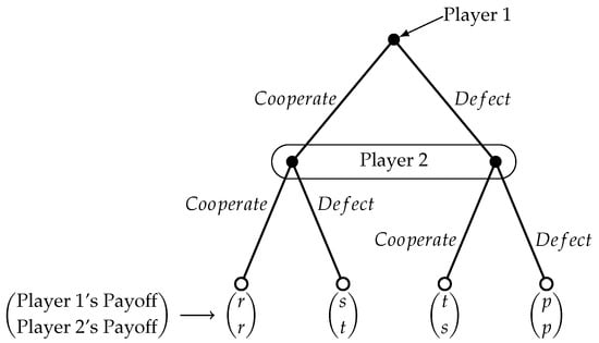
Figure 1.
An extensive form of the classical prisoner’s dilemma game. Two stages of the game are shown, but one can easily see how it evolves.
The players’ actions in the prisoner’s dilemma are represented according to the payoff matrix in Table 1 [2,25]. The symbols used are not chosen at random: r stands for reward, s for sucker’s payoff, t represents the temptation payoff, and p is for punishment. The numerical values used later are in accordance with those of Eisert et al. in [2].
If both players cooperate, they both receive the reward r, whereas if they both defect, they receive the punishment p. If player 1 defects while player 2 cooperates, then player 1 gets the temptation payoff t, while player 2 gets the “sucker’s” payoff s. Symmetrically, if 1 cooperates while 2 defects, then 1 receives the sucker’s payoff s, while 2 receives the temptation payoff t. Considering that the players are rational and care only about their individual payoff, “defect” is the dominant strategy of the game [25]. For the payoff values, it holds that , which is necessary for mutual cooperation to be superior to mutual defection for the players, and at the same time defect is guaranteed to be the dominant strategy for both players. The extensive form of the game is described using a game tree, depicted in Figure 1.
3.2. Quantum Computing Background
For a detailed description of quantum computation we refer the reader to [7]. In this paper, the sets of real and complex numbers are denoted by and , respectively, whereas denotes the set of all complex matrices. An n-dimensional vector space endowed with an inner product is called a Hilbert space [61]. Typically, the state of a quantum system is represented by a ket over a complex Hilbert space. Each ket is a superposition of the basis kets, , where |i⟩ denotes the ith basis ket, the corresponding probability amplitude, and n is the dimension of the Hilbert space. We assume that kets are normalized, i.e., . In the finite dimensional case, an operator T is just a matrix of . For every operator T, denotes its adjoint (conjugate transpose). Every observable is associated with a Hermitian operator , where Hermitian means that . Evolution among quantum states is achieved through the application of unitary operators U, that is, operators for which holds.
3.3. PD under Quantum Rules
The quantum version of rhe prisoner’s dilemma has been extensively investigated since the innovative work of Eisert et al. in [2]. It has been argued that their variant of the quantum PD game is not general enough. Nevertheless, a more general form than the EWL scheme (as suggested in [3]) would not allow a player to act in a dominant way. Such a general setup would invariably end up being equivalent to the always defect case of the classical setup. For this reason, in this work we rely on the EWL protocol. In the EWL scheme, a physical model of the prisoners’ dilemma in the context of quantum mechanics gives players the chance to escape the classical dilemma to cooperate (C) or defect (D). The players’ quantum actions are operators in a two-dimensional complex Hilbert space with basis kets . According to the work of Eisert et al. in [2], the strategic space can be represented by the following two-parameter family of operators:
where and .
Each player is given a qubit by a referee and may only act on it locally via operators chosen from the above family by picking specific values for the parameters and . In theory, the players’ states, , , can be entangled. A quantum strategy for player i is represented as an operator from the set of operators from Equation (1) (see [2]). The operator C denotes the action “cooperate,” while D describes the action “defect.”
Again, we note that the operators described in Equations (2) and (3) are based on the work of Eisert et al. in [2] (i.e., the EWL scheme), whose quantum version of the PD is the basis for the work described later.
How It Is “Quantumly” Played
The game is initialized, and each player (i.e., players 1 and 2) is given a qubit. The gate represents an operator that produces entanglement between the two qubits, and for this reason, it is usually called an entangler, where is the degree of entanglement. For no entanglement, , whereas for maximal entanglement it should be (in general, ). The actions are executed by operators and for each player, respectively. Gate is a reversible two-bit gate that “disentangles” the states. The quantum circuit that corresponds to the quantum PD is depicted in Figure 2 (initially proposed by Eisert et al. [2]).
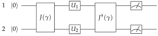
Figure 2.
A depiction of the the circuit model of the quantum prisoner’s dilemma as proposed by Eisert et al. in [2].
In quantum game theory, two quantum states and (where and are Hilbert spaces) can be entangled. In this case, the overall state of the system is described as a two-player quantum state , where and . The four basis vectors of the Hilbert space , defined as the classical game outcomes (, , , and ) [62]. These vectors are derived from the fact that Equations (2) and (3) correspond to the classical actions of cooperate and defect, respectively [2,62]. Assuming that the initial state of both players is , the unitary operator J, known to both players, entangles the two-player system (see [2,63]), leading to the state . These works showed that it is possible to have a Nash equilibrium set of actions that coincides with the Pareto optimal pair of actions, something that was impossible in the classical setting of the same game.
In the quantum version of the PD, the states of the players after the actions of cooperation or defection are represented by the two basis kets |C⟩ and |D⟩, respectively, in the Hilbert space of a two-state system. The classical action is selected by setting and , whereas the strategy is selected by setting and . The quantum action is given by . The two players choose their individual quantum actions , and and the disentangling operator acts before the measurement of the players’ state, which determines their payoff. The state prior to measurement (i.e., after each qubit is entangled and each player has applied its chosen action) is
The expected payoff depends on the payoff matrix and the joint probability of observing the four observable outcomes , and of the game [56].
with .
3.4. Repeated PD and Conditional Strategies
A classical play of the PD game (i.e., one-stage PD) has a limited range of possible strategies, since there is only one round of the game. The fact that there are only two possible actions for each player yields four possible outcomes. Thus, each player’s strategy is trivial and cannot be widely sophisticated. Therefore, the iterated or repeated variant of this game is of greater interest compared to the simple one-step setting [25]. The outcome of the first play is observed before the second stage begins. The payoff for the entire game is simply the sum of the payoffs from the two stages. This can easily be extended for n stages of the game (for ).
In a single round of the PD game, two rational individuals might not cooperate, even though it is in their mutual best interest, and subsequently they will be driven to defect. On the other hand, cooperation may be rewarded in the repeated PD. The game is repeatedly played by the same participants [64]. In the repeated PD, participants can learn about their counterpart and base their strategy on past moves with no regular convention. It is easy to show by induction that defect is the unique Nash equilibrium for the finitely repeated version of the PD game. For the scope of this paper, iterative and repeated mean the same thing. Conditional strategies are a set of rules that each player follows when deciding what action to choose, having as a condition the other player’s behavior in previous stages. For example, the altruistic “always cooperate” strategy can be exploited by the “always defect” strategy. Note that the repeated version requires that (according to the payoff as shown in Table 1) in addition to , in order to prevent the alternation of cooperation and defection that would lead to a greater reward than mutual cooperation.
3.4.1. Tit for Tat Conditional Strategy
“Tit for tat” is a common iterative prisoner’s dilemma conditional strategy (found in other games too), in which a player cooperates in the first round and then chooses the action that the opposing player has chosen in the previous round. In a repeated game, tit for tat highlights that cooperation between participants may have a more favorable outcome than a non-cooperative strategy [11,27,35,65]. The reverse tit for tat conditional strategy, proposed in [66], is a variant of the standard tit for tat, where a player defects on the first move and in consequent stages of the game plays the reverse action of the opponent’s last move.
3.4.2. Pavlov Conditional Strategy
A completely different strategy, known as the Pavlov strategy, is “win-stay, lose-shift.” A Pavlov strategy is based on the principle that if the most recent payoff was high, the same choice is repeated, otherwise the choice is changed. In its simplest form, the Pavlov sequence tends toward cooperation, unless the previous move had an unfavorable outcome (i.e., the player cooperated but the other defected). Both strategies (tit for tat and Pavlov) reinforce mutual cooperation [65,67].
3.5. Repeated Quantum PD
The repeated quantum PD game observes three rules:
- Each player has a choice to either cooperate |0⟩ , or defect |1⟩ at each round of the game.
- A unitary operator (or an action), denoted by or , respectively, is applied by each player to her qubits. Players are unable to communicate with each other.
- “Gates” are introduced to entangle the qubits. The actions of the players in the quantum game will result in a final state that will be a superposition of the basis kets. When the final state is measured, the payoff is determined from the table.
The evolutionary aspect in this repeated form of the game allows for cooperative solutions, even in the absence of communication. As discussed in [2,63], the quantum players can escape the dominant strategy to “defect.” As commented in [68], this quantum advantage can become a disadvantage when the game’s external qubit source is corrupted by a noisy “demon.”
4. Quantum Automata
Two models of quantum finite automata were initially proposed in [17,18]. The former model is known as measure-once quantum automata (meaning that a single measurement operator is applied at the end of the computation with respect to the orthonormal kets representing the automaton’s accepting states), whereas the latter is known as measure-many quantum automata (since a measurement is applied after each read symbol). A comprehensive overview of these models, along with further insights and examples, is provided in [16]. Here, we follow the measure-once paradigm.
In this section, we give the definition of -periodic quantum automata, which are inspired from the periodic quantum -automata introduced in [19]. The present definition is appropriate for the case of finite inputs. We mention in passing that despite their simplicity and their inherent limitations, periodic quantum -automata are capable of recognizing particular languages with a probability of 1. Specifically, they recognize with a probability of 1 languages of the form . That is, they recognize a language with a probability cut-point . This class of languages was described in [19,21]. For the purposes of this work, a cut-point other than (e.g., with or , which are usually discussed) would not be necessary since the game strategies can be associated to the aforementioned automata model. Measurement is performed infinitely often after the reading of input symbols (hence the term periodic) with respect to the orthonormal basis of the automaton’s states. Note that the cut-point restriction being equal to 1 could be lifted or modified, but it would not contribute anything to the purposes of this work (it would be of interest, though, in case someone is interested in probabilistic acceptance). For a deeper introduction to classical automata and computation theory, the reader is referred to [69].
If we lift the infinite character of the inputs in the previous description, then we have the -periodic quantum automata, where a single measurement is applied after reading letters. We keep the notion of periodicity in order to avoid any confusion with the standard measure-once quantum automata of [17]. Periodicity is also somehow “embedded” in the functionality of the periodic quantum automata due to the periodic-like evolution of the operators. The set P of projection matrices is the same for every automaton used later in this paper.
Definition 2.
A simple μ-periodic 1-way quantum automaton is a tuple , where Q is the finite set of states, Σ is the input alphabet, for each symbol , is the unitary matrix that describes the corresponding transitions among the states, is the initial state, μ is a positive integer that defines the measurement period, is the set of final states, and for each , is the projector to the state q.
Periodic quantum automata accept words of the form , etc., with a probability cut-point (like the infinite case). Again, measurement is performed after the reading of symbols (hence the term periodic) with respect to the orthonormal basis of the states (but this time only once, unlike the infinite case). Similarly to the definition of the infinite variant, the set P of projection matrices is the same for every automaton used later in this paper, thus it is omitted from now on.
Note that the value of the period has to be a positive integer in order for the computation to have a physical meaning (we cannot perform a measurement after reading 2.1 symbols!). For the finite case, it is obvious that the period is actually the length of the read sequence of letters, but in order to be consistent with the original definition and due to the connection with the angle factor of each read symbol, we keep the notation “periodic.”
5. Quantum Automata for the Classical Repeated PD
The classical PD game has two different actions for every player, which means that there are possible outcomes. We note again that for the purposes of the repeated version of the PD game, the outcome of the first play is observed before the second stage begins for all n stages of the game (for ). This holds for the quantum version too. The symbolic values from Table 1 can be replaced with numerical values, leading to Table 2.
Table 2.
Numerical payoff matrix for the prisoner’s dilemma game.
This corresponds to the one-stage version of the game. We represent the choice of “cooperation” with “C” and with “D”, “defection” (see Table 3). Consequently, the game’s four possible outcomes are . Then it is easy to map each one of these to a letter of the alphabet (as depicted in Table 4).
Table 3.
Representation of actions using letters.
Table 4.
Associating a letter to each possible outcome of the prisoner’s dilemma (PD) game.
Below, we present a graphical depiction of a periodic automaton like those that will be associated to repeated stages of the PD game. This is shown in Figure 3.
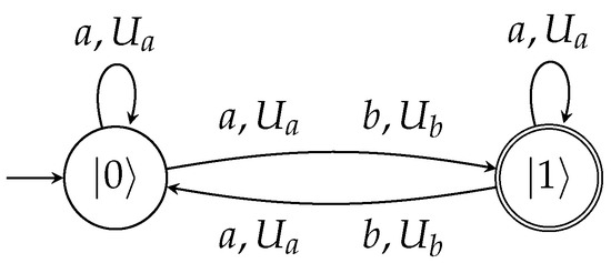
Figure 3.
A simple quantum periodic automaton inspired from the work in [19]. The measurement period is (the period is equal to the sum 4 + 1 of the exponents), and it accepts with a probability of 1 the language (or in case the input and the measurement mode is infinite, it accepts the ).
5.1. Classical Pavlov in PD and Automata
In this part, we discuss the outputs of the the repeated PD game for stages, where is an arbitrary positive integer that defines the number of plays. It is imperative to emphasize that this number is unknown to the players in order not to have a predefined series of actions [27], which would lead to a dominant strategy of always “Defect” for both of them. We follow the actions-to-letter association of Table 4. The associated automata in every case recognize the respective language with probability cut-point . We clarify that the projective measurement, with respect to the orthonormal basis of the automaton’s states, is performed after the reading of the input symbols. Furthermore, in all scenarios, the measurement period is equal to the number of stages or, equivalently, to the number of input symbols (and consequently, in the case of repeated versions of the game, ). Thus, a measurement is imposed after reading a total of symbols. But this can be easily extended to the infinite case by requiring measurements to take place periodically in time-steps after symbols are read. For example, if the accepted language is , this means that there are input symbols in total, that is, stages of the game are played, which in turn implies that .
5.1.1. Player 1 Plays Pavlov
Initially, we assume that Player 1 chooses to follow the Pavlov strategy. At first, Player 2 always defects, which means that regardless of what Player 1 chooses, Player 2 defects. As seen from the series of plays, the Pavlov strategy can be exploited by the all-defect strategy.
The regular expression for this sequence can be described as . This enables us to associate it with a variant of the quantum periodic automata that is able to recognize such languages, even if they are infinitely repeated. The automaton defined below can achieve this task.
The language is recognized with a probability of 1 by the -periodic quantum automaton that is defined as the tuple , where = , and = .
For the next scenario, we assume that Player 2 always cooperates.
The regular expression for this sequence can be described as . This leads us to associate it with a variant of the quantum periodic automata that is able to recognize such languages, even if they are infinitely repeated. The following automaton does the work.
The language is recognized with a probability of 1 by the -periodic quantum automaton that is defined as the tuple , where = .
Next, suppose that Player 2 chooses to follow the Pavlov strategy, similarly to Player 1.
For this case, the associated automaton is the same as the above (i.e., ) since the underlying language is the same, i.e., .
Next, Player 2 applies the tit for tat strategy.
Again, the associated automaton is the same as the previous one since the accepted language is .
Finally, we consider the case where Player 2 follows the reversed tit for tat strategy.
The regular expression for this sequence is , which is recognized with a probability of 1 by the -periodic quantum automaton that is defined as the tuple , where , , and .
5.1.2. Player 1 Plays Tit for Tat
In this series of PD games, we assume that Player 1 chooses to follow the tit for tat strategy, whereas Player 2 always defects.
The regular expression for this sequence is , and the corresponding -periodic quantum automaton is exactly the same as .
When Player 2 always cooperates, we have:
Its associated automaton is again the same as .
When Player 2 follows the Pavlov logic, we have:
Again, the resulting automaton is .
Then, if Player 2 applies the tit for tat strategy, we have:
The corresponding automaton is the same as .
For the scenario where Player 2 follows the reversed tit for tat strategy, we have:
In this case, the resulting automaton is a bit more complicated than those previously encountered since this series yields the regular language . With , we denote the length of the string (in this case, it is equal to 4, but we prefer to use in order to emphasize its derivation). The associated -periodic quantum automaton is the tuple , where , ,
, , and is a positive multiple of , i.e., , for some positive integer k.
For this particular scenario that seems a bit more complicated, it is important to emphasize that the measurement period has to be a multiple of the length of the substring in order to guarantee that the measurement will return an accepting outcome with a probability of 1 (as stated in the definition of -periodic quantum automata in Section 4), otherwise the acceptance cut-point is . This means that the read symbols (or the number of PD stages) have to be multiples of this length (in this case ).
5.1.3. Player 1 Plays Reversed Tit for Tat
Assuming Player 1 chooses to follow the reversed tit for tat strategy, whereas Player 2 always defects, we have:
The regular expression for this sequence is , and the associated -periodic quantum automaton is similar to by swapping the letter b with the letter d.
When Player 2 always cooperates, we have:
The associated automaton for this scenario is the same as , where the unary language is accepted with a probability of 1. For this scenario, all we have to do is to replace the letter a with c.
When the Pavlov strategy is followed by Player 2, we have:
The regular expression for this sequence is the , which is recognized with a probability of 1 by the -periodic quantum automaton that is defined as the tuple , where , , and .
When Player 2 follows tit for tat, we have the series of plays shown below.
The associated automaton for this scenario is the same as , where instead of the substring , we now have the substring . The language for this scenario is the regular language . Regarding the period , the same restrictions as those of must also hold.
Finally, if Player 2 follows the reversed tit for tat behavior, it holds that:
For this scenario, the measurement period has to be a multiple of the length of the substring in order to guarantee the desired outcome with a probability of 1. This is equivalent to saying that the number of input symbols (or the number of PD stages) must be multiples of this length (in this case ).
6. Quantum Version of Conditional Strategies
In this section, we study the quantum version of the repeated PD game. Now, each player chooses an action that is expressed as a unitary operator that acts on his own qubit. Each player has its own qubit that is entangled using the known J operator. In this case, Alice (or Player 1) has her qubit in state |0⟩ and Bob (or Player 2) has his in state |1⟩. The actions of each player are expressed using unitary operators that can take infinitely many values according to the scheme described by Eisert et al. in [2]. This scheme was criticized in [3] (to which a subsequent reply from Eisert et al. followed [70]) due to the restrictions imposed to players’ actions. Despite the fact that this limitation leads to a slightly different version of the quantum PD game, it is technically correct and has served as a basis model for several other works [5,14,33,54,71,72].
We follow the standard quantum setting of the PD game as described in the previous section of this paper (based on the EWL scheme). It is assumed that each player is informed about the other player’s choice regarding his/her chosen operator. If we combine this assumption with the previously described strategies for the classical version (like Pavlov, tit for tat, etc.), it seems like we pose restrictions on the range of the players’ actions. This is due to the fact that although the players are free to choose any action they wish in the first step, their next moves are affected by the previous moves of the other player. This leads to their response being either to continue with their previous action, to copy the other player’s move, or to “flip” the latter’s action. As a result, each player’s range of actions seemingly converges to a subset of all the possible actions.
We recall that each player’s action is expressed with a unitary operator from the two-parameter family of operators of the form
Player 1 acts via the operator and Player 2 via the operator. Like the classical version of the PD game (and generally every two-player non-cooperative game), conditional strategies like tit for tat or Pavlov are defined in a straightforward way. In this part, we consider proper alternations of the conditional strategies from the previous section, and we enrich them with new ones. Next, we proceed to the association with quantum finite automata, as we did for the classical PD.
Strategies for the Quantum PD
Here we establish the strategies for the quantum repeated PD game, and we associate them to inputs of quantum automata. First, the symbolic payoff matrix for the quantum PD game is shown in Table 5, whereas in Table 6, the numerical values for each pair of actions are depicted.
Table 5.
The payoff matrix for the quantum PD game, where players can choose to apply four different actions. C stands for cooperate, D for defect, M for the miracle move, and Q for the Q move.
Table 6.
The numerical values for the quantum PD game.
When multiple stages of a game take place and conditional strategies have to be designed, each player tries to avoid successive losses. To achieve this, Player 1 has to know the action taken by Player 2 in the previous round of the game (and vice versa). This cannot be directly observed by himself since the measurement of the state dissolves any information regarding the choices of the actions of both players. Thus, in our setting, every player announces the unitary operator they used in the previous part, and it is assumed that they are not lying about it.
As already noted, the pure classical strategies of cooperate and defect are expressed as and , where U is given by Equation (5). We observe that the cooperate operator
is the identity operator, and the defect operator
resembles the bit-flip operator.
Aside from the two classical actions, we have to introduce two purely quantum actions. The first one is the miracle action [2] that allows the player to always win against the other player’s classical strategy. The other action is the Q move, which enables the existence of a new Nash equilibrium point that is also a Pareto optimal. We associate the player’s strategies with the following unitary matrices:
7. Defining the Quantum “Disruptive” Conditional Strategy
In this part of the paper, we define the “disruptive” conditional strategy, where one players tries to disrupt the other player’s rational choices by choosing the quantum action that deviates from the Pareto optimal. This novel quantum strategy is introduced in this work for the first time and is analyzed through comparisons with other conditional strategies. The player who chooses to follow this conditional strategy is no longer rational—instead, he tries to sabotage the whole procedure. Bob assumes the role of Player 1 and Alice the role of Player 2.
Definition 3.
A disruptive (or sabotage) quantum strategy for the quantum version of the prisoner’s dilemma is defined as a series of actions by Bob , in which he starts with the unitary operator , and every time Alice chooses to use Q, he switches to for his next turn until Alice either defects, cooperates, or uses the miracle move. Then, he continues with Q until Alice again chooses Q.
A strategy is actually a rule that dictates one player’s reaction to another one’s actions. This particular strategy tries to puzzle the other player in order to disrupt his plan of action as much as possible, taking into account the fact that for most sequences of moves, the () point will be met since it is the Pareto optimal and the Nash equilibrium at the same time. Thus, Player 1 acts in a disruptive way, trying to take advantage of the fact that a rational Player 2 will strive for the Pareto optimal condition. From this observation, it is obvious that the disruptive player is actually an irrational one, aiming for the disorientation of the other player, which leads to less advantageous outcomes, even for himself. Such a strategy does not exist in the classical version of the PD game, since in that case, the Pareto point does not coincide with the Nash equilibrium. Repeated games differ from one-stage games because the players’ actions can ensure retaliation or provide them with rewards, according to their preferred strategies.
7.1. Quantum Disruptive Strategy Against Others
Similarly to the classical case, we now consider variations of the quantum game played using the disruptive strategy against straightforward quantum variants of the well-known strategies, as was done in the previous section of this paper. A quantum finite automaton is shown to accept the output for each scenario. We note that the associated automata recognize the respective language with a probability cut-point in each case. Again, measurement is performed with respect to the orthonormal basis of the automaton’s states, after input symbols are consumed by the automaton.
Player 1 Plays Disruptively
To begin with, we have to revisit the letter association to each action. Now each player applies an operator, for Player 1 and for Player 2. Each of these operators depends on two parameters and . For appropriate values of and , we have the defect and cooperate analogs of the standard versions, as well as the miracle and Q moves. Hence, the possible actions for each player as shown in Table 7 arise.
Table 7.
Representation of quantum actions using letters.
This in turn leads to Table 8, of the possible outcomes of the game (according to the payoff matrix of Table 5 and Table 7), where each possible pair of outcomes is associated with a letter.
Table 8.
Associating a letter to each possible outcome of the quantum PD game.
We note that for some particular pairs of actions, there are two or more possible outcomes due to the probabilistic nature of the quantum game. Therefore, conditional strategies are affected by the measurement outcome. For the examples below, we choose an arbitrary value of every possible outcome.
Assuming Player 1 chooses to follow the “disruptive” quantum strategy, whereas Player 2 always defects, we have:
The automaton for this scenario is the same as , where the unary language is accepted with a probability of 1. For this scenario, all we have to do is to replace the letter a with d (that is, ).
In the following scenario, Player 2 always cooperates.
Again, we have a similar association with a previous automaton, in particular . This time, the language is . This is not unexpected considering the quite simplistic strategy chosen by Player 2.
Next, Player 2 always uses the miracle move.
Again, we have a similar association with . This time, the language is .
Next, Player 2 always chooses the Q move.
This series yields the language . The corresponding -periodic quantum automaton is similar to .
If Player 2 follows the classical Pavlov strategy (meaning that he begins with cooperate), we have:
This series yields the language . The associated -periodic quantum automaton is the tuple , where = , = , and = .
Next, Player 2 again uses the Pavlov strategy, but this time he starts with Q instead of C. Then we have:
This series yields the language , which is the same as the -periodic quantum automaton .
Next, Player 2 follows the classical tit for tat, that is, he starts with cooperate.
This series yields the language , which is identical to the one accepted by the -periodic quantum automaton .
Suppose now that Player 2 follows the tit for tat strategy starting with the Q move.
This series of plays yields the language , and the corresponding automaton is .
Finally, in the following scenario, Player 2 uses the reversed tit for tat strategy, where he responds with cooperation to defection (and vice versa) and the miracle move to the Q move (and vice versa).
This series yields the language , which is similar to , accepted by the automaton, where instead of the letters a and i, we now have d and f, respectively.
7.2. Changing the Action to C when the Other Played M
In this part, we propose an even “more disruptive” strategy, where Player 1 not only responds with an M move to the other player’s Q, but he also responds with a C move to the other player’s M. Similarly to the previous scenarios, we begin with the setting where Player 2 always defects.
The corresponding automaton is similar to a previous one, specifically, . This time the language is .
Next, Player 2 always cooperates:
Again, we have an association with the automaton, since the language is .
In the same manner, below there is the setting where Player 2 always applies the miracle move.
Again, we meet a mirror of the automaton, now for the language .
When Player 2 always applies the Q move, we have:
which again yields the association with the automaton, this time for .
Things get more interesting when Player 2 is forced to follow the Pavlov strategy (with initial cooperation). In this case, we have:
This again leads to the association with the automaton, this time for .
When Player 2 follows the Pavlov strategy (with initial Q move), we have:
Once again, the resulting automaton is , this time for (as in other scenarios).
Then, Player 2 follows the tit for tat strategy, choosing to cooperate as a first move.
This series yields the language , where is the length of the substring . The associated -periodic quantum automaton is the tuple , where = , = , = , = , and = .
For this particular scenario, the measurement period has to be a multiple of the length of the substring for the measurement to return an accepting outcome with a probability of 1. This means that the read symbols (or the number of PD stages) have to be multiples of this length (in this case, ).
If Player 2 chooses tit for tat with Q as an initial move, we have the following sequences.
In this scenario, the language is similar to the previous one, thus, it is associated to the same automaton , only now modified to accept the language .
Finally, for the next scenario, Player 2 chooses the reversed tit for tat (swapping actions for C/D and M/Q, starting action is irrelevant).
For this case, the language is , which is quite similar to the one accepted by the automaton, which was designed for the language.
7.3. Remarks on the “Disruptive” Conditional Strategy and the Use of Automata
In the previous section, we analyzed the evolution of the quantum PD game when it is repeatedly played, and we tested the proposed “disruptive” quantum strategy in contrast to other pro-cooperation quantum strategies, like quantum tit for tat, etc. These strategies (always cooperate, always defect, quantum tit for tat, quantum Pavlov, and quantum reversed tit for tat) were simply the quantum analogues of the standard ones, whereas new ones had to be introduced (always miracle action and always Q action).
At first, we observe that the proposed strategy leads to a low level of disruption for the player who chooses to follow it against the always defect strategy, whereas it does not seem to have any impact when always cooperate is followed by the other player. This highlights the fact that the disruptive strategy can have no effect when the other player has purely cooperative purposes and does not care for rational actions. This also holds in case Player 2 follows the always miracle action. For these two scenarios, the disruptive strategy is weak, but we note that since the quantum PD game as presented in [2] has a Nash pair of actions , the disruptive player assumes that the other player would rationally choose the Q move. That is the reason for choosing the EWL model of the quantum PD, since the more general one as proposed in [3] could not serve the purposes of the disruptive conditional strategy (there would not be any rational strategy to “disrupt”).
On the other hand, the quantum disruptive conditional strategy fails to complete its mission for both quantum versions of Pavlov, which is not surprising given Pavlov’s character. Against the quantum tit for tat versions, there is a balance regarding the gains for each player, which also holds for the quantum reversed tit for tat. When the disruptive player becomes more disruptive in Section 7.2, we now have a better result for Player 1 when he competes against the always miracle and always Q strategies (i.e., disruption is achieved). Player 1 has also better results against the quantum Pavlov case, whereas for the tit for tat case, the results are roughly the same as in the simple disruptive policy.
The advantages of using the proposed association with quantum periodic automata means that we are able to validate consecutive plays of the quantum PD game using a computational mechanism that is highly efficient when it comes to the number of states. This result is in accordance with other works from the literature (like [19,23,24]). It has also become clear that a disruptive policy that might be followed by an irrational player can be addressed using other well-known conditional strategies. Efficient computational mechanisms that can verify such claims, probably for more complex scenarios, are always important, and this work lies in this exact direction.
8. Conclusions
Game theory constitutes a broad research area that can be divided into many subfields and branches. When infused with traces of quantum computation (or more generally, quantum mechanics), then we may speak of quantum game theory. The effort to “quantize” classical games is gaining more and more attention in the quest for challenging game-theoretic results, like better Nash equilibria pairs of actions. The well-known prisoner’s dilemma problem is one of the most studied games, and its quantum analogue has already been proposed [1,2,5,21,42]. Since then, it has attracted a lot of attention due to some interesting and counter-intuitive results, like the coincidence of a Pareto optimal point with a Nash equilibrium point for particular instances of this game.
The repeated versions of these games, especially in the classical setting, have also been under the spotlight for various reasons. Trying to shed more light onto their quantum analogues, in this paper we have introduced and analyzed the conditional quantum strategies. The most dominant are the tit for tat and the Pavlov. Repeated games differ from simple games of one stage, since in the former case, the players’ actions can lead to retaliation or reward through appropriate strategic choices (some of them favor cooperation and others do not).
In this work, we also propose a new conditional strategy that is applied in the quantum setup of the prisoner’s dilemma game. This “disruptive” quantum strategy is defined, and subsequently, its behavior is compared against other strategies that are properly adjusted to fit in the quantum frame of the game. It is shown that under particular circumstances, this strategy is able to confuse the other player, under the assumption that Player 2 follows some known conditional strategy. Finally, the outcomes of these scenarios, along with scenarios from the classical setting of the PD game, are associated to a variant of quantum automata, namely the periodic quantum automata, which emphasizes the connection among formal methods of state machines with aspects of game theory.
We expect this association to prove quite handy in analyzing distinct plays by players using compact computation schemes since the periodic quantum automata, albeit weak regarding the recognizing spectrum, are small in size. The results presented in this paper should be useful to anyone studying the repeated version of the quantum PD, providing some noteworthy material and new insights for particular cases. In general, having quantum automata that are able to process and decide inputs related to the repeated form of the PD could have an impact on evaluating such conditional strategies efficiently and in a sophisticated way.
Author Contributions
Conceptualization, K.G. and T.A.; Formal analysis, K.G., G.T., and T.A.; Methodology, K.G. and S.F.; Software, C.P.; Supervision, T.A.; Validation, C.P. and S.F.; Writing—original draft, K.G. and G.T.; Writing—review & editing, K.G., G.T., C.P., S.F., and T.A.
Funding
This research is funded in the context of the project “Investigating alternative computational methods and their use in computational problems related to optimization and game theory” (MIS 5007500) under the call for proposals “Supporting researchers with an emphasis on young researchers” (EDULL34). The project is co-financed by Greece and the European Union (European Social Fund, ESF) by the operational program Human Resources Development, Education and Lifelong Learning 2014–2020.
Conflicts of Interest
The authors declare no conflict of interest.
Abbreviations
The following abbreviations are used in this manuscript:
| EWL scheme | Eisert–Wilkens–Lewenstein scheme (from [2]) |
| PD | Prisoner’s dilemma |
| RPD | Repeated prisoner’s dilemma |
| C | Cooperate |
| D | Defect |
References
- Meyer, D.A. Quantum Strategies. Phys. Rev. Lett. 1999, 82, 1052–1055. [Google Scholar] [CrossRef]
- Eisert, J.; Wilkens, M.; Lewenstein, M. Quantum games and quantum strategies. Phys. Rev. Lett. 1999, 83, 3077. [Google Scholar] [CrossRef]
- Benjamin, S.C.; Hayden, P.M. Comment on “Quantum Games and Quantum Strategies”. Phys. Rev. Lett. 2001, 87, 069801. [Google Scholar] [CrossRef] [PubMed]
- Jiménez, E. Quantum games: Mixed strategy Nash’s equilibrium represents minimum entropy. Entropy 2003, 5, 313–347. [Google Scholar] [CrossRef]
- Khan, F.S.; Solmeyer, N.; Balu, R.; Humble, T.S. Quantum games: A review of the history, current state, and interpretation. Quantum Inf. Process. 2018, 17, 309. [Google Scholar] [CrossRef]
- Feynman, R.; Vernon, F., Jr. The theory of a general quantum system interacting with a linear dissipative system. Ann. Phys. 1963, 24, 118–173. [Google Scholar] [CrossRef]
- Nielsen, M.A.; Chuang, I.L. Quantum Computation and Quantum Information; Cambridge University Press: Cambridge, UK, 2010. [Google Scholar]
- Von Neumann, J.; Morgenstern, O. Theory of Games and Economic Behavior (Commemorative Edition); Princeton University Press: Princeton, NJ, USA, 2007. [Google Scholar]
- Osborne, M.J.; Rubinstein, A. A Course in Game Theory; MIT Press: Cambridge, MA, USA, 1994. [Google Scholar]
- Smith, J.M.; Price, G.R. The logic of animal conflict. Nature 1973, 246, 15. [Google Scholar] [CrossRef]
- Nowak, M.A.; Sigmund, K. Evolutionary dynamics of biological games. Science 2004, 303, 793–799. [Google Scholar] [CrossRef]
- Hammerstein, P.; Hagen, E.H. The second wave of evolutionary economics in biology. Trends Ecol. Evol. 2005, 20, 604–609. [Google Scholar] [CrossRef]
- Moretti, S.; Vasilakos, A.V. An overview of recent applications of Game Theory to bioinformatics. Inf. Sci. 2010, 180, 4312–4322. [Google Scholar] [CrossRef]
- Alonso-Sanz, R. Quantum Approach to Game Theory. In Quantum Game Simulation; Springer International Publishing: Cham, Switzerland, 2019; pp. 11–19. [Google Scholar]
- Khan, F.S.; Phoenix, S.J. Gaming the quantum. arXiv 2012, arXiv:1202.1142. [Google Scholar]
- Ambainis, A.; Yakaryılmaz, A. Automata and quantum computing. arXiv 2015, arXiv:1507.01988. [Google Scholar]
- Moore, C.; Crutchfield, J.P. Quantum automata and quantum grammars. Theor. Comput. Sci. 2000, 237, 275–306. [Google Scholar] [CrossRef]
- Kondacs, A.; Watrous, J. On the power of quantum finite state automata. In Proceedings of the 38th Annual Symposium on Foundations of Computer Science, Miami Beach, FL, USA, 20–22 October 1997; pp. 66–75. [Google Scholar]
- Giannakis, K.; Papalitsas, C.; Andronikos, T. Quantum automata for infinite periodic words. In Proceedings of the 2015 6th International Conference on Information, Intelligence, Systems and Applications (IISA), Corfu, Greece, 6–8 July 2015; pp. 1–6. [Google Scholar]
- Bhatia, A.S.; Kumar, A. Quantum ω-Automata over Infinite Words and Their Relationships. Int. J. Theor. Phys. 2019, 58, 878–889. [Google Scholar] [CrossRef]
- Giannakis, K.; Papalitsas, C.; Kastampolidou, K.; Singh, A.; Andronikos, T. Dominant Strategies of Quantum Games on Quantum Periodic Automata. Computation 2015, 3, 586–599. [Google Scholar] [CrossRef]
- Tian, Y.; Feng, T.; Luo, M.; Zheng, S.; Zhou, X. Experimental demonstration of quantum finite automaton. Npj Quantum Inf. 2019, 5, 4. [Google Scholar] [CrossRef]
- Ambainis, A. Superlinear advantage for exact quantum algorithms. SIAM J. Comput. 2016, 45, 617–631. [Google Scholar] [CrossRef]
- Gruska, J.; Qiu, D.; Zheng, S. Potential of quantum finite automata with exact acceptance. Int. J. Found. Comput. Sci. 2015, 26, 381–398. [Google Scholar] [CrossRef]
- Maschler, M.; Solan, E.; Zamir, S. Game Theory; Cambridge University Press: Cambridge, UK, 2013. [Google Scholar] [CrossRef]
- Mathieu, P.; Delahaye, J.P. New Winning Strategies for the Iterated Prisoner’s Dilemma. J. Artif. Soc. Soc. Simul. 2016, 20. [Google Scholar] [CrossRef]
- Axelrod, R.; Hamilton, W.D. The evolution of cooperation. Science 1981, 211, 1390–1396. [Google Scholar] [CrossRef]
- Hilbe, C.; Traulsen, A.; Sigmund, K. Partners or rivals? Strategies for the iterated prisoner’s dilemma. Games Econ. Behav. 2015, 92, 41–52. [Google Scholar] [CrossRef] [PubMed]
- Maynard Smith, J. Evolution and the Theory of Games; Cambridge University Press: Cambridge, UK, 1982. [Google Scholar]
- Wedekind, C.; Milinski, M. Human cooperation in the simultaneous and the alternating Prisoner’s Dilemma: Pavlov versus Generous Tit-for-Tat. Proc. Natl. Acad. Sci. USA 1996, 93, 2686–2689. [Google Scholar] [CrossRef] [PubMed]
- Rubinstein, A. Finite automata play the repeated prisoner’s dilemma. J. Econ. Theory 1986, 39, 83–96. [Google Scholar] [CrossRef]
- Abreu, D.; Rubinstein, A. The structure of Nash equilibrium in repeated games with finite automata. Econom. J. Econom. Soc. 1988, 56, 1259–1281. [Google Scholar] [CrossRef]
- Landsburg, S. Nash equilibria in quantum games. Proc. Am. Math. Soc. 2011, 139, 4423–4434. [Google Scholar] [CrossRef]
- Dyer, M.; Mohanaraj, V. The Iterated Prisoner’s Dilemma on a cycle. arXiv 2011, arXiv:1102.3822. [Google Scholar]
- Axelrod, R.; Dion, D. The further evolution of cooperation. Science 1988, 242, 1385–1390. [Google Scholar] [CrossRef] [PubMed]
- Mittal, S.; Deb, K. Optimal strategies of the iterated prisoner’s dilemma problem for multiple conflicting objectives. IEEE Trans. Evol. Comput. 2009, 13, 554–565. [Google Scholar] [CrossRef]
- Golbeck, J. Evolving strategies for the prisoner’s dilemma. Adv. Intell. Syst. Fuzzy Syst. Evol. Comput. 2002, 2002, 299. [Google Scholar]
- Gossner, O.; Hernández, P.; Peretz, R. The complexity of interacting automata. Int. J. Game Theory 2016, 45, 461–496. [Google Scholar] [CrossRef]
- Andronikos, T.; Sirokofskich, A.; Kastampolidou, K.; Varvouzou, M.; Giannakis, K.; Singh, A. Finite Automata Capturing Winning Sequences for All Possible Variants of the PQ Penny Flip Game. Mathematics 2018, 6, 20. [Google Scholar] [CrossRef]
- Sousa, P.B.; Ramos, R.V. Multiplayer Quantum Games and Its Application As Access Controller in Architecture of Quantum Computers. Quantum Inf. Process. 2008, 7, 125–135. [Google Scholar] [CrossRef][Green Version]
- Dajka, J.; Kłoda, D.; Łobejko, M.; Sładkowski, J. Quantum two player game in thermal environment. PLoS ONE 2015, 10, e0134916. [Google Scholar] [CrossRef][Green Version]
- Flitney, A.P. Review of quantum game theory. In Game Theory: Strategies, Equilibria, and Theorems; Nova Science Publishers: Hauppauge, NJ, USA, 2009. [Google Scholar]
- Du, J.; Xu, X.; Li, H.; Zhou, X.; Han, R. Playing prisoner’s dilemma with quantum rules. Fluct. Noise Lett. 2002, 2, R189–R203. [Google Scholar] [CrossRef]
- Siopsis, G.; Balu, R.; Solmeyer, N. Quantum prisoners’ dilemma under enhanced interrogation. Quantum Inf. Process. 2018, 17, 144. [Google Scholar] [CrossRef]
- Deng, X.; Zhang, Q.; Deng, Y.; Wang, Z. A novel framework of classical and quantum prisoner’s dilemma games on coupled networks. Sci. Rep. 2016, 6, 23024. [Google Scholar] [CrossRef] [PubMed]
- Li, A.; Yong, X. Entanglement guarantees emergence of cooperation in quantum prisoner’s dilemma games on networks. Sci. Rep. 2014, 4, 6286. [Google Scholar] [CrossRef][Green Version]
- Yong, X.; Sun, H.; Li, J. Entanglement plays an important role in evolutionary generalized prisoner’s dilemma game on small-world networks. In Proceedings of the 2016 IEEE Advanced Information Management, Communicates, Electronic and Automation Control Conference (IMCEC), Xi’an, China, 3–5 October 2016; pp. 319–324. [Google Scholar] [CrossRef]
- Li, A.; Yong, X. Emergence of super cooperation of prisoner’s dilemma games on scale-free networks. PLoS ONE 2015, 10, e0116429. [Google Scholar] [CrossRef] [PubMed]
- Cheon, T. Altruistic contents of quantum prisoner’s dilemma. Europhys. Lett. (EPL) 2005, 69, 149–155. [Google Scholar] [CrossRef][Green Version]
- Alonso-Sanz, R. A quantum prisoner’s dilemma cellular automaton. Proc. R. Soc. A Math. Phys. Eng. Sci. 2014, 470, 20130793. [Google Scholar] [CrossRef]
- Abal, G.; Donangelo, R.; Fort, H. Conditional quantum walk and iterated quantum games. arXiv 2006, arXiv:quant-ph/0607143. [Google Scholar]
- Bolonek-Lasoń, K. General quantum two-player games, their gate operators, and Nash equilibria. Prog. Theor. Exp. Phys. 2015, 2015. [Google Scholar] [CrossRef][Green Version]
- Frąckiewicz, P. Quantum repeated games revisited. J. Phys. A Math. Theor. 2012, 45, 085307. [Google Scholar] [CrossRef]
- Frąckiewicz, P. Quantum Games with Unawareness. Entropy 2018, 20, 555. [Google Scholar] [CrossRef]
- Marinatto, L.; Weber, T. A quantum approach to static games of complete information. Phys. Lett. A 2000, 272, 291–303. [Google Scholar] [CrossRef]
- Hanauske, M.; Bernius, S.; Dugall, B. Quantum game theory and open access publishing. Phys. A Stat. Mech. Its Appl. 2007, 382, 650–664. [Google Scholar] [CrossRef]
- Szopa, M. How Quantum Prisoner’s Dilemma Can Support Negotiations; Optimum. Studia Ekonomiczne: Bialystok, Poland, 2014. [Google Scholar]
- Chen, K.Y.; Hogg, T.; Huberman, B.A. Behavior of Multi-Agent Protocols Using Quantum Entanglement. In Proceedings of the AAAI Spring Symposium: Quantum Interaction, Stanford, CA, USA, 26–28 March 2007; pp. 1–8. [Google Scholar]
- Faigle, U.; Grabisch, M. Game theoretic interaction and decision: A quantum analysis. Games 2017, 8, 48. [Google Scholar] [CrossRef]
- Turocy, T.; Stengel, B. Game Theory-CDAM Research Report LSE-CDAM-2001-09; Centre for Discrete and Applicable Mathematics, London School of Economics & Political Science: London, UK, 2001; p. 12. [Google Scholar]
- Kreyszig, E. Introductory Functional Analysis with Applications; Wiley: New York, NY, USA, 1989; Volume 81. [Google Scholar]
- Hanauske, M.; Kunz, J.; Bernius, S.; König, W. Doves and hawks in economics revisited: An evolutionary quantum game theory based analysis of financial crises. Phys. A Stat. Mech. Its Appl. 2010, 389, 5084–5102. [Google Scholar] [CrossRef]
- Eisert, J.; Wilkens, M. Quantum games. J. Mod. Opt. 2000, 47, 2543–2556. [Google Scholar] [CrossRef]
- Arechar, A.; Kouchaki, M.; Rand, D. Examining Spillovers between Long and Short Repeated Prisoner’s Dilemma Games Played in the Laboratory. Games 2018, 9, 5. [Google Scholar] [CrossRef]
- Nowak, M.; Sigmund, K. A strategy of win-stay, lose-shift that outperforms tit-for-tat in the Prisoner’s Dilemma game. Nature 1993, 364, 56. [Google Scholar] [CrossRef]
- Nachbar, J.H. Evolution in the finitely repeated prisoner’s dilemma. J. Econ. Behav. Organ. 1992, 19, 307–326. [Google Scholar] [CrossRef]
- Kraines, D.; Kraines, V. Pavlov and the prisoner’s dilemma. Theory Decis. 1989, 26, 47–79. [Google Scholar] [CrossRef]
- Johnson, N.F. Playing a quantum game with a corrupted source. Phys. Rev. A 2001, 63, 020302. [Google Scholar] [CrossRef]
- Sipser, M. Introduction to the Theory of Computation; Thomson Course Technology: Boston, MA, USA, 2006; Volume 2. [Google Scholar]
- Eisert, J.; Wilkens, M.; Lewenstein, M. Eisert, Wilkens, and Lewenstein Reply. Phys. Rev. Lett. 2001, 87, 069802. [Google Scholar] [CrossRef]
- Vlachos, P.; Karafyllidis, I.G. Quantum game simulator, using the circuit model of quantum computation. Comput. Phys. Commun. 2009, 180, 1990–1998. [Google Scholar] [CrossRef]
- Frąckiewicz, P. Strong isomorphism in Eisert-Wilkens-Lewenstein type quantum games. Adv. Math. Phys. 2016, 2016, 1–8. [Google Scholar] [CrossRef]
© 2019 by the authors. Licensee MDPI, Basel, Switzerland. This article is an open access article distributed under the terms and conditions of the Creative Commons Attribution (CC BY) license (http://creativecommons.org/licenses/by/4.0/).