An Automated ECG Beat Classification System Using Deep Neural Networks with an Unsupervised Feature Extraction Technique

Abstract

An automated classification system based on a Deep Learning (DL) technique for Cardiac Disease (CD) monitoring and detection is proposed in this paper. The proposed DL architecture is divided into Deep Auto-Encoders (DAEs) as an unsupervised form of feature learning and Deep Neural Networks (DNNs) as a classifier. The objective of this study is to improve on the previous machine learning technique that consists of several data processing steps such as feature extraction and feature selection or feature reduction. It is also noticed that the previously used machine learning technique required human interference and expertise in determining robust features, yet was time-consuming in the labeling and data processing steps. In contrast, DL enables an embedded feature extraction and feature selection in DAEs pre-training and DNNs fine-tuning process directly from raw data. Hence, DAEs is able to extract high-level of features not only from the training data but also from unseen data. The proposed model uses 10 classes of imbalanced data from ECG signals. Since it is related to the cardiac region, abnormality is usually considered for an early diagnosis of CD. In order to validate the result, the proposed model is compared with the shallow models and DL approaches. Results found that the proposed method achieved a promising performance with 99.73% accuracy, 91.20% sensitivity, 93.60% precision, 99.80% specificity, and a 91.80% F1-Score. Moreover, both the Receiver Operating Characteristic (ROC) curve and the Precision-Recall (PR) curve from the confusion matrix showed that the developed model is a good classifier. The developed model based on unsupervised feature extraction and deep neural network is ready to be used on a large population before its installation for clinical usage.

1. Introduction

Artificial Intelligence (AI) techniques have been widely used to improve the quality of patient life and care through early diagnosis of disease. Such a technique has become popular because it not only can reduce cost-effectiveness and mortality, but also provides good predictions that facilitate precise treatment [1,2,3]. Cardiac Disease (CD) monitoring and detection, in particular, is a difficult task which requires identifying the patterns and interaction among variables using various techniques [2]. Despite these significant efforts, recently it has been shown that conventional methods based on a simple score do not perform well and the results obtained by such methods remain unsatisfactory to date. The application of computer-based methods is a potential solution that allows cardiologists to observe the CD in the long-term recording with the better-diagnosing result. However, to produce an optimal CD prediction requires some metrics such as sensitivity, specificity, and accuracy. These parameters help the cardiologist to predict outcomes accurately and effectively. They cannot only be evaluated using a simple score (i.e., probability and statistical method) or traditional CD risk factors (i.e., diabetes, hypertension, and smoking). Currently, Machine Learning (ML) algorithms can overcome the drawbacks of automatic learning to help build a recommendation system. The results can help a medical doctor or cardiologist in making more accurate and sensitive predictions [2,3,4].

The learning process is an important stage of ML algorithms in order to produce accurate diagnosis and prediction. It generally can be categorized into three types of learning processes: supervised, unsupervised, and reinforcement. In supervised learning, algorithms use a dataset labeled by experts. The algorithms develop a model to predict or classify future events or to determine which variables are most relevant to the outcome. ML with supervised learning produces excellent results in classification and regression problems [5]. However, it requires a lot of data to be labeled by humans, and it is time-consuming [5]. In contrast, unsupervised learning seeks to identify novel disease mechanisms from hidden patterns present in the data without feedback from humans. Unfortunately, it always produces some bias, due to in the initial cluster patterns not being validated with other groups of data [6]. The combination process between supervised and unsupervised learning is called reinforcement learning. However, to obtain high accuracy, the reinforcement learning process needs a trial and error phase, which is a very time-consuming, and it can also produce untrustworthy results [3,5]. Hence, an improvement in the learning process to produce high performance with trusted values is desirable.

There are three phases to process CD prediction using an ML algorithm: training, validation, and testing. Unfortunately, with less training data sets, CD prediction can lead to inaccurate predictions in the testing phase, meaning it can be biased and inaccurate [6]. In order to improve the diagnosis results, more data sets are required for training the model [2,6]. Deep learning (DL) is one of the ML approaches which has been successfully implemented in a diverse range of biomedical fields with large datasets, as presented in references [7,8]. This approach has become a promising field and has been proliferating in recent years [9,10]. DL architecture mimics human brain operation using multiple layers of the artificial neuron for generating automated predictions [5,9,10].

The DL architecture with an unsupervised learning approach has been widely implemented. It can facilitate the exploration of novel factors in score systems or add hidden risk factors to existing models [11], classify novel genotypes and phenotypes from heterogeneous cardiac diseases [2], detect lymph node metastases from breast cancer [12], detect cardiomyopathy [13], and use a risk factor prediction of bleeding and stroke to provide the optimal dose and anticoagulant therapy duration and to identify additional stroke risk factors [14]. In the diagnosis of cardiac disease, the implementation of DL produces good results [1,5,10]. The algorithms provide a very in-depth analysis for an artificial real-time cardiac imaging with better spatial and temporal resolution. It potentially improves the quality of health caring and reducing costs [15,16,17,18,19]. Such algorithms can be trained using an unsupervised learning approach with unlimited memory [9,20,21] and, it is also suitable for noisy data [5,15,16].

Unfortunately, there are some challenges using DL such as (i) A Nonlinear training in deep learning involves a large number of parameters and layers, if it is not handled properly, it can cause overfitting on the model so that the predictions performances are poor. (ii) The analysis requires a graphical processing unit to accelerate the computation; (iii) Parameters set-up for a deep learning method architecture is also time-consuming; and (iv) Multiple layers may increase the training time without providing any improvement in precision and accuracy. Hence, selecting the most suitable DL architecture with several parameters a necessary area to study to help produce the best results in the diagnosis and prediction of cardiac disease.

2. Deep Learning

Deep Neural Networks (DNNs) with a back-propagation algorithm has limitations in specific applications as has been reported in reference [9] and reference [10]. This is because the DNNs with back-propagation is not appropriate for deeper networks. In addition, there are two main drawbacks in term of the learning process: (1) The DNNs model always falls into local minima due to a random weight initialization at the early of the training process; (2) most data is unlabeled when DNNs was initialized with the random requirement for labeled the set of data [9]. Today, such problems have been solved through the groundbreaking work of Geoffrey Hinton and his colleagues in 2006 [22]. Their research contribution, called unsupervised greedy layer-wise pre-training, is an effective solution for overcoming the problems with traditional backpropagation [20,21]. Auto-Encoder (AE) is the one method which can learn generic features using greedy layer-wise training. The process is fast and provides outstanding results on deep network architectures for classification and prediction problems [22]. Moreover, we can construct a deep AE model in order to improve performance. Besides, a deep AE model sets the training target to fit the input data. Then, the back-propagation algorithm is trained by feeding the input and calculating the error between reconstructed input and original one.

2.1. Deep Auto Encoder

Feature extraction is an important phase in the learning process to obtain appropriate and robust features. If feature quality is low, it may lead to low performance and poor generalization properties, despite having powerful classification algorithms. Some of these powerful feature extraction techniques including Principal Component Analysis (PCA) or the Linear Discriminant Analysis (LDA) algorithm. However, this method cannot extract directly from the network structure, and it usually required a trial-and-error process which is time-consuming [23,24]. By using AE, extracting features of the raw input data can work automatically. Automatically extracted features improve the performance of predictive models while at the same time reducing the complexity of the function design task. AE consists of an encoder and decoder; the encoder has the same function in DNNs by transforming the input vector to a hidden layer representation with a weight matrix and bias/offset vector. Simultaneously, the decoder maps the hidden layer representation of the reconstructed input, which is regarded as the output result.

A dimensionality reduction process on AE was done by extracting low-dimensional features from high-dimensional spectral envelopes in a non-linear and unsupervised way. An input vector is assumed to be $\overline{x}$, a hidden representation vector $\overline{y}$, and the reconstruction vector $\overline{z}$. The reconstruction and update flow can be represented by the encoder and decoder process. In this step, the hidden weight and the bias vector are $\overline{W}$ and $\overline{b}$ respectively, while the outputs are $\overline{W}\prime$ and $\overline{b}\prime$ respectively. The function $\sigma$ is an activation function and $\eta$ is the learning rate. A deterministic mapping function called the encoder is $y=f_{\theta }(x)=\sigma (W_x+b)$, then a reverse mapping function called the decoder is $z=g_{\theta }(y)=\sigma (W\prime y+b\prime )$. The weight parameter is usually constrained at $W\prime =W^T$. The parameter of AE can be trained by minimizing the following objective function as follows [25,26,27]:

$$\theta ,\theta \prime ={}_{\theta ,\theta \prime }{}^{\arg \min }\frac{1}{n}{\displaystyle {\sum }_{i=1}^{n}L(x_i,z_i)}$$

(1)

$${}_{\theta ,\theta \prime }{}^{\arg \min }\frac{1}{n}{\displaystyle {\sum }_{i=1}^{n}L}(x_i,g_{\theta },(f_{\theta }(x_i)))$$

(2)

where L is a cost function, and the mean square error (MSE) is used,

$$L(x_i,z_i)=\parallel x_i-z_i{\parallel }^2$$

(3)

For each ECG signal input x, the hidden representation y of the kth feature map is represented by,

$$y^k=\sigma (W^{K}x+b^k)$$

(4)

2.2. Proposed Deep Learning Structure

The proposed DL architecture is divided into Deep Auto-Encoders (DAEs) pre-training and DNNs fine-tuning phases, as presented in Figure 1. The fully connected layer is added on top of the encoder part of the DAEs. Figure 1 describes a conceptual depiction of the classifier architecture of the pre-trained DAEs model. In some case of the pre-training process, the DAEs structure can be stacked to improve the quality of signal reconstruction and to obtain effective initial parameters for the fine-tuning via unsupervised learning. However, if the pre-training produces a good performance in data reconstruction, the encoder output can directly be used as an input into the classifier, and the weights can be fine-tuned using back-propagation. The computational resources and an enormous amount of data are required for learning in both phases.

The classifiers are trained with input $x$, and output is annotated as a label. The Softmax function is used for the output layer of the classifier as an activation function. The output of each unit can be treated as the probability of each label using the Softmax function [25,26,27]. Let $N$ be the number of units of the output layer, $x$ as the input, and $x_i$ as the output of unit $i$. Then, the output $p(i)$ of unit $I$ is defined by Equation (5),

$$p(i)=\frac{e^{xi}}{{\displaystyle \sum _{j=1}^N{e}^{xj}}}$$

(5)

Cross entropy is used as the loss function of the classifier $L_f$ as follow,

$$L_f(\theta )=-\frac{1}{n}{\displaystyle \sum _{i=1}^n{\displaystyle \sum _{j=1}^m{y}_{ij}\log (p_{ij})}}$$

(6)

where $n$ is the sample size, $m$ is the number of classes, $p_{ij}$ is the output of the classifier of class $j$ of the $i_{th}$ sample and $y_{ij}$ is the annotated label of class $j$ of the $i_{th}$ sample.

3. Experimental Result

3.1. Data Preparation

The raw ECG datasets used in the present study are available in the MIT repository (https://physionet.org/physiobank/database/mitdb/) [28,29]. All of the ECG beat data is annotated at R-peak locations, and there are up to 16 different types of arrhythmias. Under the AAMI standard [29], the database contains 22 types of beats within 5 groups of arrhythmias. However, only 10 types are used in this study [10,23,30]. There are 10 types of ECG beats, i.e., normal (N), atrial premature contraction (A), premature ventricular contraction (V), right bundle branch block (R), left bundle branch block (L), paced (P), ventricular flutter wave (!), fusion of ventricular and normal (F), fusion of paced and normal (f) and nodal escape (j), and all data sets for 10 types of ECG beats are presented in

Table 1. The classes of arrhythmia and the number of samples.

Label	Description of Beats	Count
		Training	Testing
A	Atrial premature contraction	2316	230
L	Left bundle branch block	7222	850
N	Normal	67545	7477
P	Paced	6315	710
R	Right bundle branch block	6528	727
V	Premature ventricular contraction	6411	718
f	Fusion of paced and normal	884	98
F	Fusion of ventricular and normal	724	78
!	Ventricular flutter wave	422	50
j	Nodal escape	213	16

.

3.2. Segmentation and Reconstruction

Automatic beats segmentation of the ECG using a minimum heuristic a priori information is an essential problem in the clinical diagnosis of heart disease. The various segments of the ECG have different physiological meanings, and the presence, timing, and duration of each of these segments all have diagnostic and bio-physical importance. The former refers to the features extracted from a single beat, which usually contains only one beat. The raw data sample of the ECG rhythm signal in the normal condition is illustrated in Figure 2a. The normal rhythm is segmented into one beat by determining the P wave, QRS complex and T wave, which are directly related to the R-peak location. The segmentation on an ECG signal is presented in Figure 2b. In general, the frequency of the ECG rhythm is between 60 and 80 per minute [15]. The process segmentation to find the R position after the R position is detected, and the sampling is conducted at about 0.7-second segment for one beat. The segment is divided into two intervals, t₁ of 0.25-s before peak position (R) and the interval t₂ of 0.45-s after the peak position (R) (see Figure 2b). All generated nodes during 0.7-s are about 252 nodes, which divided into two intervals, 90 nodes for t₁ and 162 nodes for t₂. The result of the sampling process illustration is shown in Figure 2c.

After the segmentation process, DAEs used to extract features from the beat automatically. From Figure 2, the DAEs works based on two processes, i.e., compressing and reconstructing. The compressing means the encoder decreases the dimensionality of the input up to the layer with the fewest neurons, called latent space. The reconstructing means the decoder then tries to reconstruct the input from this low-dimensional representation. This way, the latent space forms a bottleneck, which forces the DAEs to learn an effective compression method for the data. In this study, four different topologies are considered and are the following: [252 - 32 - 252], [252 - 128 - 64 - 32 - 64 - 128 - 252], [252 - 128 - 64 - 32 -16 - 32 - 64 - 128 - 252], and reference [252 - 128 - 64 - 32 - 16 - 8 – 16 - 32 - 64 - 128 - 252]. All of these can be interpreted as performing a lossy compression whose ratio is 8:1. The possible activation functions are ReLU and Sigmoid. Each DAEs is optimized via Adam with α = 0.0001. In this study, the parameter of the learning rate is changing from 0.1 to 0.0001, and the smallest loss value becomes the baseline to select the learning rate. The loss function uses MSE without any regularization terms, and training epochs are considered to be at 100. Finally, before being fed to the DAEs, all data are scaled to [−1, 1]. This step is min-max normalization with the minimum and the maximum being given by the minimum and maximum values in the training set. It can be seen in Figure 3 that the normal and right bundle branch block beat (RBBB) is utilized as a sample of the ECG signal after segmentation and reconstruction. Figure 3a,c described the initial signal ECG and the output of the DAEs. The raw data produce some noise in high and low frequency, and it is cancelled by DAEs after reconstruction, as presented in Figure 3b,d.

3.3. Classifier Structure

The proposed DL architecture was constructed by combining the pre-trained DAEs encoding layer and fine-tuned of DNNs part with the fully connected layer. In the classifier part used ReLU as the activation function, Cross-entropy as the loss function and Adam as the optimization method with the learning rate is set from 0.1 and gradually decreased to 0.0001. Adam optimization allows the use of adaptive learning rates for each parameter. The result of learning rate used is that the learning rate about 0.001 produces a good result in the loss value. Figure 1 shows the details of the proposed structure for the fully connected classifier. We have used 10 experiments to select the best model structure of deep learning (see

Table 2. Processing time of 10 DL structures.

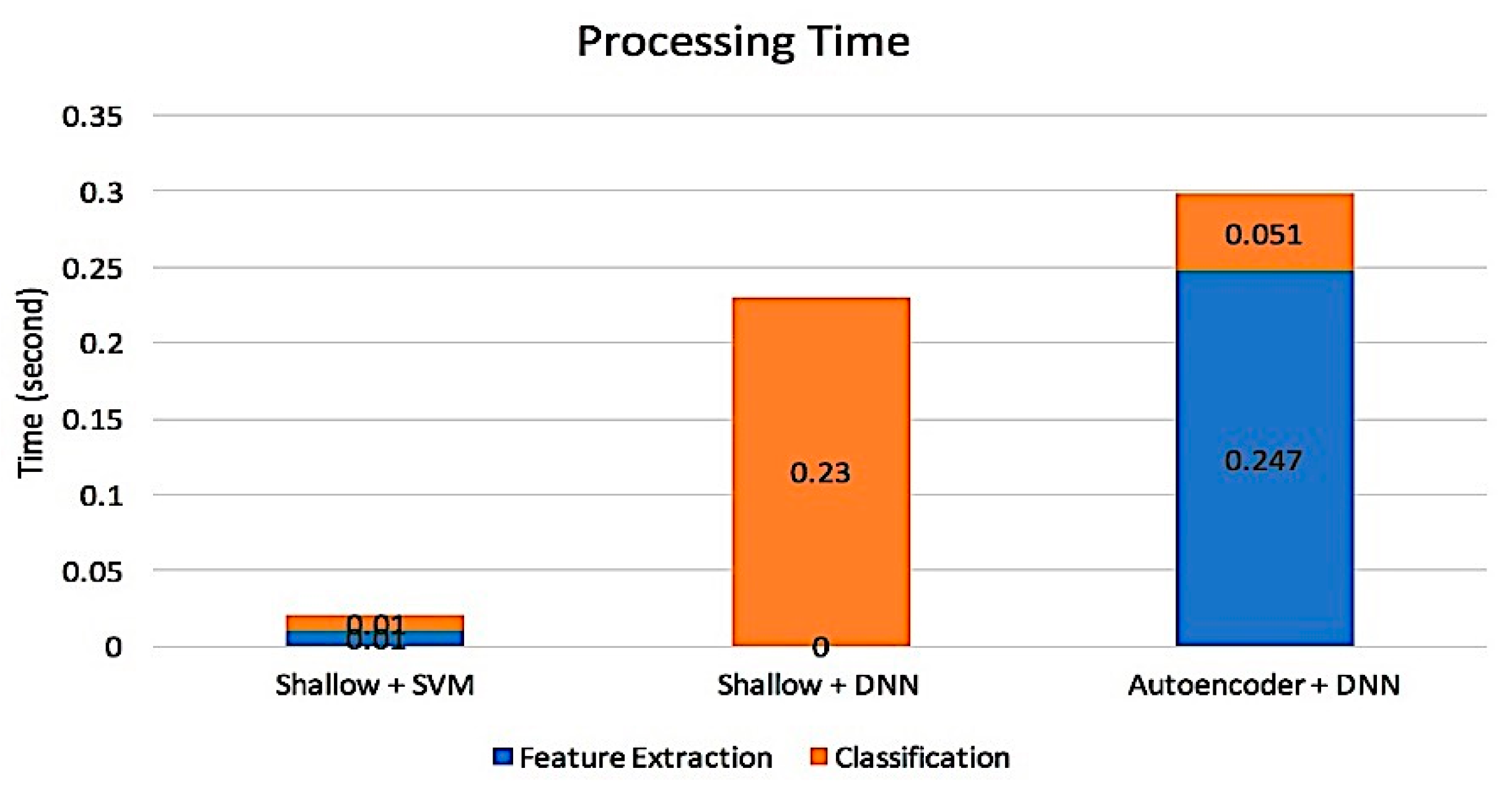
Model	Feature Learning Structure	DAEs Training Time (s)	Classifier Structure	DNNs Training Time (s)	Proces-Sing Time (s)	DNNs Testing Time (s)
1	Auto-Encoder (252 - 32 - 252)	991.07	MLP (32 - 100 - 10)	243.46	1234.53	0.08
2	Auto-Encoder (252 - 32 - 252)	991.07	DNN 2 HLs (32 - 100 - 50 -10)	280.94	1272.01	0.1
3	Auto-Encoder (252 - 32 - 252)	991.07	DNN 3 HLs (32 - 100 - 50 - 100 - 10)	313.33	1304.41	0.1
4	Auto-Encoder (252 - 32 - 252)	991.07	DNN 4 HLs (32 - 100 - 50 - 100 - 50 - 10)	327.84	1318.92	0.13
5	Auto-Encoder (252 - 32 - 252)	991.07	DNN 5 HLs (32 - 100 - 50 - 100 - 50 - 100 - 10)	354.68	1345.75	0.42
6	Deep Auto-Encoder (252 - 128 - 64 - 32 - 64 - 128 - 252)	1866.67	MLP (32 - 100 - 10)	241.24	2107.91	0.08
7	Deep Auto-Encoder (252 - 128 - 64 - 32 - 64 - 128 - 252)	1866.67	MLP 2 HLs (32 - 100 - 50 - 10)	273.55	2140.22	0.09
8	Deep Auto-Encoder (252 - 128 - 64 - 32 - 64 - 128 - 252)	1866.67	DNN 3 HLs (32 - 100 - 50 - 100 - 10)	315.34	2182.01	0.10
9	Deep Auto-Encoder (252 - 128 - 64 - 32 - 64 - 128 - 252)	1866.67	DNN 4 HLs (32 - 100 - 50 - 100 - 50 - 10)	353.26	2219.93	0.12
10	Deep Auto-Encoder (252 - 128 - 64 - 32 - 64 - 128 - 252)	1866.67	DNN 5 HLs (32 - 100 - 50 - 100 - 50 - 100 - 10)	381.51	2248.18	0.14

). All parameters were tuned to obtain the smallest loss value to avoid overfitting, high accuracy, high sensitivity, high specificity, high precision, and high F1-Score. However, the deep structure must produce a short processing time and small memory usage. Table 2 shows that DL performance improved when using a ReLU activation function, compared to the Sigmoid activation function. Moreover, ReLU activation function was a more straightforward computation than sigmoidal functions, and it has been proven that ReLU works better than sigmoidal functions [31]. Based on all performances, model 8 was selected as the best model with three hidden layers in pre-training and three hidden layers of fine-tuning used. In our work, model 8 is the proposed DL structure in

Table 3. The proposed structure of deep learning of model 8.

Method	Input Layer	Output Layer	Hidden Layer Neuron	Activation Function Hidden	Activation Function Output	Learning Rate	Loss Function	Batch Size
DAEs Pre-Training	252	252	128-64-32-64-128	ReLU	Sigmoid	0.0001	MSE	8
DNNs Fine-Tuning	32	10	100-50-50-50-100	ReLU	Softmax	0.001	Cross-Entropy	32

. Table 3 shows the proposed structure of the deep learning method used in the present study.

3.4. Results

Figure 4a–c illustrates the data distribution among the classes. It can be seen that the initial ECG data distribution, which consists of 252 features representing a raw ECG signal, was unstructured and imbalanced; therefore, it can influence one another. In order to minimize the complexity of the data by reducing data dimensionality, PCA and DAEs are used and compared. PCA is one of the main linear dimensionality reduction techniques for extracting effective features from high dimensions’ data, while DAEs is nonlinear techniques. The nonlinear techniques have an advantage over linear techniques for solving the problems of the real-world because real-world data are nonlinear in nature like medical data. From the previous research, it is observed that the nonlinear techniques are performing better than linear techniques on artificial tasks and succeed in overcoming poor natural datasets [25,27].

In this study, DAEs reduced the feature from 252 into 32 features while PCA with a cumulative energy value of 0.99, the initial feature is lowered to 32 features for 10 (ten) classes. It can be seen in Figure 4b,c that there is a significant difference between the DAEs and PCA in terms of data distribution plots. By using PCA, it is assumed that the data lie on or near a linear subspace of the high-dimensional space. However, DAEs do not rely on the linearity assumption as a result of which more complex embedding of the data in the high-dimensional space. Therefore, the data distribution from PCA remains unstructured, and it is centered at a certain point, hence it is challenging to discriminate data patterns from each class. DAEs, on the other hand, produces a better data distribution. Its feature distribution becomes clearer so that the minority classes are not polarized with larger classes.

Moreover, DAEs was able to eliminate spikes from the original signal without losing the information in the ECG signal and was also able to learn nonlinear feature representations, as presented in Figure 4. All colors in Figure 4a–c respectively, show 10 (ten) classes of Arrhythmia such as N, A, V, R, L, P, !, F, f , and j.

To obtain an optimum classification performance, various DL structures in the learning process were examined. Ten structures were determined and validated prior to the selection of the best model. All classifiers were arranged in two processes: training and testing. The processing time was investigated in our model because the structure must embeddable in the hardware as an ECG interpretation module for further application. All processing time results of 10 DL structures are presented in Table 2.

From Table 2, the experiment describes training time for feature learning, classifier, and testing time. In this case, the trade-off happened between model complexity and processing time. It worth noting that the processing time increases with a more complex DL structure. However, a smaller architecture is better for feasible application on the real-time system. Hence, we selected the DAEs architecture with 5 layers combined with DNNs with 3 hidden layers (model 8). It produces a good performance in terms of accuracy, sensitivity, specificity, precision, and F1-score compare to the other structures. As presented in Table 2, a 10 structures model validation of DNNs with a DAEs feature learning model are selected for further analysis.

Such a process was done by changing the number of neurons and the number of hidden layers, activation functions, and cost functions of DAEs and DNNs structures. The training process uses 80% of the data, and the testing process uses the remaining data percentage. The validation phase for all models is presented in

Table 4. Training performances based on 10 models.

Training	Model Validation (%)
Metrics	1	2	3	4	5	6	7	8	9	10
Accuracy	99.23	99.63	99.83	99.83	99.78	99.74	99.80	99.90	99.64	99.55
Sensitivity	70.73	84.69	92.80	89.57	93.79	90.55	92.31	94.10	83.41	80.70
Specificity	99.07	99.61	99.83	99.80	99.82	99.77	99.80	99.90	99.60	99.50
Precision	81.85	94.77	95.79	96.97	93.39	94.98	94.49	97.43	93.55	91.80
F1-Score	75.26	88.38	94.10	91.98	93.54	92.27	93.26	95.70	84.48	84.00

, and

Table 5. Testing performances based on 10 models.

Testing	Model Validation (%)
Metrics	1	2	3	4	5	6	7	8	9	10
Accuracy	99.22	99.55	99.71	99.74	99.64	99.62	99.68	99.73	99.58	99.52
Sensitivity	69.25	82.00	88.29	86.06	90.18	86.36	89.97	91.20	80.72	80.41
Specificity	99.08	99.54	99.72	99.71	99.69	99.67	99.68	99.80	99.55	99.46
Precision	80.46	91.37	90.32	94.12	88.88	89.26	89.26	93.60	94.97	93.35
F1-Score	73.78	85.75	89.26	88.59	89.45	87.63	89.78	91.80	80.93	85.38

, respectively. Table 4 shows the results from the various DL structures in the training process. Based on validation model 8 in Table 3, the training and testing process produces the best performance metrics to all classes (see Table 4 and Table 5). The training process produces 99.9% accuracy, 94.1% sensitivity, 99.9% specificity, 97.4% precision and a 95.7% F1-Score, while in the testing process produce 99.7% accuracy, 91.2% sensitivity, 99.6% specificity, 93.6% precision and a 91.8% F1-Score.

The confusion matrix was applied to analyze model prediction on each class during the training and the testing process.

Table 6. Confusion matrix for the training process.

Class	A	L	N	P	R	V	F	F	!	j
A	2086	3	210	0	14	0	0	0	0	3
L	0	7222	0	0	0	0	0	0	0	0
N	39	10	67412	0	10	44	2	6	0	22
P	0	0	1	6303	0	1	10	0	0	0
R	11	0	4	0	6511	2	0	0	0	0
V	2	5	29	0	0	6354	0	20	1	0
f	1	2	38	6	0	3	832	0	0	2
F	2	1	73	0	0	35	0	613	0	0
!	0	0	4	1	0	4	0	1	412	0
j	1	0	47	0	4	0	0	0	0	161

and

Table 7. Confusion matrix for testing process.

Class	A	L	N	P	R	V	f	F	!	j
A	190	0	37	0	0	1	0	0	0	2
L	0	847	1	0	0	1	0	1	0	0
N	7	1	7449	0	2	13	1	0	0	4
P	0	0	0	707	0	0	3	0	0	0
R	4	0	2	0	720	1	0	0	0	0
V	0	5	10	1	0	693	0	4	5	0
f	1	1	7	1	0	0	87	1	0	0
F	0	1	15	0	0	7	0	54	1	0
!	0	1	0	0	0	2	0	0	47	0
j	0	0	3	0	0	0	0	0	0	13

present the predicted class only for model 8 as the best model. According to Table 6, less than 5% of the ECG heartbeats are misclassified in the training and testing process. This is because of imbalanced data, and the F1-Score needed due to it was able to describe trusted data from our model. From our best model, the F1-scores were 95.70% and 91.80% for training and testing, respectively (see Table 7).

In order to validate the proposed DL structure, accuracy, and loss curve is presented in Figure 5 and Figure 6. It is shown in Figure 5a,b that the errors from training and testing data were decreased along with the increasing epochs. Both diagrams produce good shapes since the DAEs has the ability to extract high-level of features not only from the training data but also from the unseen data. In addition, The DAEs reconstruction result shows the effect of noise cancelation while maintaining its overall shape (see Figure 4).

For a metric scheme, the values of sensitivity and specificity will change along with the cutoff value. In every cutoff value, a dot can be plotted using the coordinate (Specificity, Sensitivity). A curve that connects all these dots is called a Receiver Operating Characteristics (ROC) curve. The ROC curve which is far away above the diagonal, especially in the upper-left corner, produces the right predictions with random guesses. However, if the dataset is highly imbalanced, the shape of the ROC curve is biased and may be misleading [32,33]. The MIT BIH arrhythmia dataset is imbalanced, due to the higher number of normal figures compared to disorderly ones. Therefore, in this paper, the Precision-Recall (P-R) curve is used to overcome the limitation of the ROC curve. The larger area under the curve (AUC) in P-R curve indicates a better performance. Every value in the confusion matrix is related to the ROC and P-R curve. The values in both curves give the same performance in this study. All the values produced a better performance as a classifier by using the proposed model (see Figure 6).

4. Discussion

The nonlinear processing in the stacked of multiple layers is well suited to capturing highly varied functions with the conciseness of the parameters set. Based on unsupervised pre-training, DL allows assigning deeper networks in a parameter space region to avoid local minima. The availability of large sets or even with only a small number of data, DL techniques achieves excellent performance, and often the best one. Due to only a few studies using DL in arrhythmia classification, several experiments were designed to benchmark our proposed model.

We have selected several ML methods to benchmark our model, and the result is compared in terms of accuracy, sensitivity, specificity, precision, and F1-score (see

Table 8. Selected method for the benchmarking proposed method.

Classifier	Accuracy (%)	Precision (%)	Sensitivity (%)	Specificity (%)	F1-Score (%)
Random Forest + PCA	98.85	87.21	60.00	98.30	66.89
SVM + PCA + DWT	99.76	98.30	97.22	99.69	97.94
DL with SAE	99.52	90.70	86.68	99.45	81.70
DNNs + PCA + DWT	99.76	98.20	91.80	99.78	97.80
DL (proposed method)	99.73	93.60	91.20	99.80	91.80

and

Table 9. Selected literatures for benchmarking our proposed model.

No	Classifier	Accuracy (%)	Sensitivity (%)	Specificity (%)	Precision (%)	F1 –Score (%)
1	CNN [17]	92.70	-	-	-	-
2	DBN [36]	98.60	88.00	99.25	-	-
3	DBN and SAE [20]	90.20	51.03	82.76	-	-
4	CNN [16]	-	78.4	-	80.00	77.60
5	CNN [15]	89.05	95.90	88.37	-	-
6	CNN [19]	99.39	-	-	-	-
7	RNN [31]	91.33	-	-	-	-
8	RBM and DBN [37]	94.60	-	-	-	-
9	DNN [38]	99.68	99.48	99.83	-	-
10	RNN [39]	88.10	92.40	83.35	-	-
11	CNN and RNN [40]	83.40	-	-	-	-
12	CNN [18]	93.91	93.93	94.19	-	-
13	DEEP CODED FEATURES and LSTM [41]	99.23	-	-	-	-
14	Our DL Model	99.73	91.20	99.80	93.60	91.80

) [34,35,36]. From Table 8, shallow architecture like SVM and DNNs produce a good performance, but from all results, a DNNs model with PCA and DWT produces high performance, such as accuracy of about 99.76%, precision of about 98.20%, sensitivity of about 91.80%, specificity of about 99.78% and an F1-measure of about 97.80%. However, feature extraction in shallow architecture is very difficult; it must be processed separately and manually. On the other hand, DL has a feature learning approach. It learns the feature directly from the network by using its structure. Such an approach can be used as both dimensionality reduction and noise cancelation. It reduces the time process and gives a simpler procedure with a big and imbalanced data set. As a result found that DL performances are lower compared with the SVM and DNNs counterpart, in terms of precision about 93.60% and F1-Measure about 91.80% (DL with DAEs). However, the advantage of DL is that it does not require a human to identify and compute the critical features. DL learns discriminatory features that best predict the outcomes. This prediction means that the amount of human effort required to train DL systems is less (because no feature engineering or computation is required) and may also lead to the discovery of important new features that were not anticipated. In addition, due to its ability to learn critical feature directly from data, even with highly imbalanced data, the learned features are still robust enough to discriminate the class labels. Moreover, from Table 9, our proposed architecture is compared with other DL performances. However, many previous studies calculate only 3 metrics without the F1 Score and precision, whereas in the medical data, especially in Arrhythmia, the data set is imbalanced. Therefore, the complete metrics to measure the prediction must be calculated. It can be shown that our proposed DL model based on DAEs and DNNs are leading with others DL like CNN, DBN, and RNN. The DL produces accuracy of about 99.73%, sensitivity of about 91.20%, specificity of about 99.80%, precision of about 93.60%, and an F1-Score of about 91.80%.

In addition, to analyze memory usage and the speed of processing time, a comparison between DL architecture and Shallow Architecture was conducted. Figure 7 and Figure 8 illustrate that the shallow architecture with an SVM classifier produces fast processing time and less memory usage. However, by using shallow architecture, the process of feature extraction and feature reduction was manually engineered without considering the low-level feature from the data. This requires more time and effort to investigate the stage. Thus, only the best value is selected to obtain excellent performance. In this study, the comparison three classifiers i.e., DNNs, SVM, and DL are presented. According to the experimental result, it is found that the SVM classifier with PCA and DWT produce the best result that what, as presented in Table 8. Unfortunately, when a large data set is used, the SVM performance is decreased. This problem occurred because the SVM classifier is cost-inefficient when an extensive data set is applied. This was mostly a small data set problem. Therefore, the DL classifier will provide promising things in the future because the data will be increased over time.

5. Conclusions

A deep learning approach is presented in this study to automatically learning and classifying the 10 class of ECG heartbeats, which is important for the diagnosis of cardiac arrhythmia. While dealing with a highly variable function which requires a large number of labeled samples, the DL Architecture expresses its full potential. However, training deep architectures is a challenging task. The shallow architecture has provided a good result. Unfortunately, shallow architectures are not as efficient as deep architectures. Adding more layers does not necessarily lead to better solutions and choosing the correct dimensions of a deep architecture is not an easy task. In this research, unsupervised learning for DAEs pre-training is combined with a supervised fine-tuned deep neural structure. Several models are designed to obtain the best classifier, by changing the number of neurons, the number of hidden layers, learning rate value, optimizer, activation function, and loss function. The best value is selected based on validation data in several cases of ECG signal. In addition, the classes are highly imbalanced; the amount of each class has very different sizes. Our proposed architecture, the combination of DAEs and DNNs structure, gives a better performance compared to the other selected DL approach. The DL produces 99.73% accuracy, 91.20% sensitivity, 99.80% specificity, 93.60% precision and a 91.80% F1-Score on the testing data. In the future, to overcome the limitations of cardiologists and to develop broader ECG devices, we hope that this technology will be incorporated into inexpensive ECG devices as diagnostic tools everywhere.

References

- Erickson, B.J.; Korfiatis, P.; Kline, T.L.; Akkus, Z.; Philbrick, K.; Weston, A.D. Deep learning in radiology: Does one size fit all? J. Am. Coll. Radiol. 2018, 15, 521–526. [Google Scholar] [CrossRef] [PubMed]
- Krittanawong, C.; Zhang, H.; Wang, Z.; Aydar, M.; Kitai, T. Artificial intelligence in precision cardiovascular medicine. J. Am. Coll. Cardiol. 2017, 69, 2657–2664. [Google Scholar] [CrossRef] [PubMed]
- Larrañaga, P.; Calvo, B.; Santana, R.; Bielza, C.; Galdiano, J.; Inza, I.; Lozano, J.A.; Armañanzas, R.; Santafé, G.; Pérez, A.; et al. Machine learning in bioinformatics. Brief. Bioinform. 2006, 7, 86–112. [Google Scholar] [CrossRef] [PubMed] [Green Version]
- Darmawahyuni, A.; Nurmaini, S.; Sukemi; Caesarendra, W.; Bhayyu, V.; Rachmatullah, M.N.; Firdaus. Deep Learning with a Recurrent Network Structure in the Sequence Modeling of Imbalanced Data for ECG-Rhythm Classifier. Algorithms 2019, 12, 118. [Google Scholar] [CrossRef]
- Al Rahhal, M.M.; Bazi, Y.; AlHichri, H.; Alajlan, N.; Melgani, F.; Yager, R.R. Deep learning approach for active classification of electrocardiogram signals. Inf. Sci. 2016, 345, 340–354. [Google Scholar] [CrossRef]
- Cunningham, P.; Carney, J. Diversity versus quality in classification ensembles based on feature selection. In Proceedings of the European Conference on Machine Learning, Barcelona, Spain, 31 May–2 June 2000; pp. 109–116. [Google Scholar]
- Le, N.-Q.-K.; Ho, Q.-T.; Ou, Y.-Y. Incorporating deep learning with convolutional neural networks and position specific scoring matrices for identifying electron transport proteins. J. Comput. Chem. 2017, 38, 2000–2006. [Google Scholar] [CrossRef] [PubMed]
- Le, N.Q.K.; Huynh, T.-T.; Yapp, E.K.Y.; Yeh, H.-Y. Identification of clathrin proteins by incorporating hyperparameter optimization in deep learning and PSSM profiles. Comput. Methods Programs Biomed. 2019, 177, 81–88. [Google Scholar] [CrossRef] [PubMed]
- LeCun, Y.; Bengio, Y.; Hinton, G. Deep learning. Nature 2015, 521, 436–444. [Google Scholar] [CrossRef]
- Nurmaini, A.G.S.; Partan, R.U.; Rachmatullah, M.N. Cardiac Arrhythmias Classification Using Deep Neural Networks and Principal Component Analysis Algorithm. Int. J. Adv. Soft Comput. Appl. 2018, 10, 14–32. [Google Scholar]
- Krumholz, H.M. Big data and new knowledge in medicine: The thinking, training, and tools needed for a learning health system. Health Aff. 2014, 33, 1163–1170. [Google Scholar] [CrossRef]
- Golden, J.A. Deep learning algorithms for detection of lymph node metastases from breast cancer: Helping artificial intelligence be seen. JAMA 2017, 318, 2184–2186. [Google Scholar] [CrossRef] [PubMed]
- Sengupta, P.P.; Huang, Y.M.; Bansal, M.; Ashrafi, A.; Fisher, M.; Shameer, K.; Gall, W.; Dudley, J.T. Cognitive machine-learning algorithm for cardiac imaging: A pilot study for differentiating constrictive pericarditis from restrictive cardiomyopathy. Circ. Cardiovasc. Imaging 2016, 9, e004330. [Google Scholar] [CrossRef] [PubMed]
- Wang, Y.; Wang, L.; Rastegar-Mojarad, M.; Moon, S.; Shen, F.; Afzal, N.; Liu, S.; Zeng, Y.; Mehrabi, S.; Sohn, S.; et al. Clinical information extraction applications: A literature review. J. Biomed. Inform. 2018, 77, 34–49. [Google Scholar] [CrossRef] [PubMed]
- Acharya, U.R.; Oh, S.L.; Hagiwara, Y.; Tan, J.H.; Adam, M.; Gertych, A.; Tan, R.S. A deep convolutional neural network model to classify heartbeats. Comput. Biol. Med. 2017, 89, 389–396. [Google Scholar] [CrossRef] [PubMed]
- Rajpurkar, P.; Hannun, A.Y.; Haghpanahi, M.; Bourn, C.; Ng, A.Y. Cardiologist-level arrhythmia detection with convolutional neural networks. arXiv 2017, arXiv:1707.01836. [Google Scholar]
- Zubair, M.; Kim, J.; Yoon, C. An automated ECG beat classification system using convolutional neural networks. In Proceedings of the 2016 6th international conference on IT convergence and security (ICITCS), Prague, Czech Republic, 26–29 September 2016; pp. 1–5. [Google Scholar]
- Sellami, A.; Hwang, H. A robust deep convolutional neural network with batch-weighted loss for heartbeat classification. Expert Syst. Appl. 2019, 122, 75–84. [Google Scholar] [CrossRef]
- Yıldırım, Ö.; Pławiak, P.; Tan, R.S.; Acharya, U.R. Arrhythmia detection using deep convolutional neural network with long duration ECG signals. Comput. Biol. Med. 2018, 102, 411–420. [Google Scholar] [CrossRef] [PubMed]
- Majumdar, A.; Ward, R. Robust greedy deep dictionary learning for ECG arrhythmia classification. In Proceedings of the 2017 International Joint Conference on Neural Networks (IJCNN), Anchorage, AK, USA, 14–19 May 2017; pp. 4400–4407. [Google Scholar]
- Bengio, Y.; Lamblin, P.; Popovici, D.; Larochelle, H. Greedy layer-wise training of deep networks. In Proceedings of the 19th International Conference on Neural Information Processing Systems, NIPS’06, Vancouver, BC, Canada, 4–7 December 2006; pp. 153–160. [Google Scholar]
- Hinton, G.E.; Osindero, S.; Teh, Y.-W. A fast learning algorithm for deep belief nets. Neural Comput. 2006, 18, 1527–1554. [Google Scholar] [CrossRef]
- Nurmaini, S.; Partan, R.U.; Rachmatullah, M.N. Deep classifiers on the electrocardiogram interpretation system. Sriwijaya International Conference on Medical and Sciences. J. Phys Conf. Ser. 2019, 1246. [Google Scholar] [CrossRef]
- Martis, R.J.; Acharya, U.R.; Min, L.C. ECG beat classification using PCA, LDA, ICA and discrete wavelet transform. Biomed. Signal Process. Control 2013, 8, 437–448. [Google Scholar] [CrossRef]
- Wang, Y.; Yao, H.; Zhao, S. Auto-encoder based dimensionality reduction. Neurocomputing 2016, 184, 232–242. [Google Scholar] [CrossRef]
- Javadi, M.; Arani, S.A.A.A.; Sajedin, A.; Ebrahimpour, R. Classification of ECG arrhythmia by a modular neural network based on mixture of experts and negatively correlated learning. Biomed. Signal Process. Control 2013, 8, 289–296. [Google Scholar] [CrossRef]
- van der Maaten, L.; Postma, E.; den Herik, J. Dimensionality reduction: A comparative. J. Mach. Learn. Res. 2009, 10, 66–71. [Google Scholar]
- Goldberger, A.L.; Amaral, L.A.; Glass, L.; Hausdorff, J.M.; Ivanov, P.C.; Mark, R.G.; Mietus, J.E.; Moody, G.B.; Peng, C.K.; Stanley, H.E. PhysioBank, PhysioToolkit, and PhysioNet: Components of a new research resource for complex physiologic signals. Circulation 2000, 101, e215–e220. [Google Scholar] [CrossRef] [PubMed]
- Moody, G.B.; Mark, R.G. The impact of the MIT-BIH arrhythmia database. IEEE Eng. Med. Biol. Mag. 2001, 20, 45–50. [Google Scholar] [CrossRef] [PubMed]
- Darmawahyuni, A. Coronary Heart Disease Interpretation Based on Deep Neural Network. Comput. Eng. Appl. J. 2019, 8. [Google Scholar] [CrossRef]
- Yildirim, Ö. A novel wavelet sequence based on deep bidirectional LSTM network model for ECG signal classification. Comput. Biol. Med. 2018, 96, 189–202. [Google Scholar] [CrossRef] [PubMed]
- Saito, T.; Rehmsmeier, M. The precision-recall plot is more informative than the ROC plot when evaluating binary classifiers on imbalanced datasets. PLoS ONE 2015, 10, e0118432. [Google Scholar] [CrossRef]
- Jiao, Y.; Du, P. Performance measures in evaluating machine learning based bioinformatics predictors for classifications. Quant. Biol. 2016, 4, 320–330. [Google Scholar] [CrossRef] [Green Version]
- Le, N.-Q.-K.; Ho, Q.-T.; Ou, Y.-Y. Classifying the molecular functions of Rab GTPases in membrane trafficking using deep convolutional neural networks. Anal. Biochem. 2018, 555, 33–41. [Google Scholar] [CrossRef]
- Le, N.-Q.-K.; Ou, Y.-Y. Prediction of FAD binding sites in electron transport proteins according to efficient radial basis function networks and significant amino acid pairs. BMC Bioinform. 2016, 17, 298. [Google Scholar] [CrossRef] [PubMed]
- Qin, Q.; Li, J.; Zhang, L.; Yue, Y.; Liu, C. Combining low-dimensional wavelet features and support vector machine for arrhythmia beat classification. Sci. Rep. 2017, 7, 6067. [Google Scholar] [CrossRef] [PubMed]
- Mathews, S.M.; Kambhamettu, C.; Barner, K.E. A novel application of deep learning for single-lead ECG classification. Comput. Biol. Med. 2018, 99, 53–62. [Google Scholar] [CrossRef] [PubMed]
- Sannino, G.; de Pietro, G. A deep learning approach for ECG-based heartbeat classification for arrhythmia detection. Futur. Gener. Comput. Syst. 2018, 86, 446–455. [Google Scholar] [CrossRef]
- Singh, S.; Pandey, S.K.; Pawar, U.; Janghel, R.R. Classification of ECG Arrhythmia using Recurrent Neural Networks. Procedia Comput. Sci. 2018, 132, 1290–1297. [Google Scholar] [CrossRef]
- Swapna, G.; Soman, K.P.; Vinayakumar, R. Automated detection of cardiac arrhythmia using deep learning techniques. Procedia Comput. Sci. 2018, 132, 1192–1201. [Google Scholar]
- Yildirim, O.; Baloglu, U.B.; Tan, R.-S.; Ciaccio, E.J.; Acharya, U.R. A new approach for arrhythmia classification using deep coded features and LSTM networks. Comput. Methods Programs Biomed. 2019, 176, 121–133. [Google Scholar] [CrossRef] [PubMed]