Deep Learning Resolves Representative Movement Patterns in a Marine Predator Species

Abstract

The analysis of animal movement from telemetry data provides insights into how and why animals move. While traditional approaches to such analysis mostly focus on predicting animal states during movement, we describe an approach that allows us to identify representative movement patterns of different animal groups. To do this, we propose a carefully designed recurrent neural network and combine it with telemetry data for automatic feature extraction and identification of non-predefined representative patterns. In the experiment, we consider a particular marine predator species, the southern elephant seal, as an example. With our approach, we identify that the male seals in our data set share similar movement patterns when they are close to land. We identify this pattern recurring in a number of distant locations, consistent with alternative approaches from previous research.

1. Introduction

The analysis of animal telemetry data can help researchers identify locations popular to animals, called biological hotspots, and to clarify movement patterns that could improve outcomes of conservation programs protecting vulnerable wildlife [1,2]. Movement analysis is also important for studying animals’ search strategies and their behavioural ecology [3]. In addition, because animals obtain resources (prey, mates, etc.) through movements, their movement patterns reveal important information on species fitness [4].

Given that the study of animal movement through telemetry technologies started more than 30 years ago, there now exists a wealth of data on animal movement [5]. Recent advances in the development of tracking technologies along with improved data analysis and visualisation techniques have dramatically changed how researchers can study the movements of free-ranging animals. Increased cross-disciplinary collaborations between mathematicians and ecologists have led to the development of new quantitative approaches and tools that have become pivotal in the study of animal movement and have allowed enhanced and broad interpretation of results [3].

Recent analysis demonstrates that marine animal subgroups could have very different movement patterns. Some research suggests that there could be more uncertainty in determining the target locations of young, inexperienced individuals [3]. Other studies observed that the preferences of female seals for locations with mesoscale oceanic circulation are seasonally flexible [6]. Moreover, ocean currents can also impact a marine animal’s motion patterns [7], and elephant seals typically forage near the edges of eddies or temperature fronts. On the other hand, pregnant female elephant seals prefer to forage near mesoscale fronts, perhaps to reduce inter-species competition [8].

In this work, we propose a novel learning model, called a recurrent neural network (RNN) with confidence measure (RNN-CM), to analyze telemetry data. Our RNN-CM approach can identify unique segments corresponding to certain animal subgroups with confidence scores. As illustrated in Figure 1, for given inputs, segments with low confidence are common segments for all the subgroups, and those with high confidence are unique segments for particular subgroups.

2. Related Work

Deep learning is a subfield of machine learning. Based on artificial neural networks, deep learning is able to learn representations of data with multiple levels of abstraction and has significantly improved the state-of-the-art in many areas [9]. For example, in hyperspectral data classification, a deep stacked autoencoder model can obtain useful high-level features and provide competitive performance [10]. In image classification and object recognition, deep convolutional neural network based approaches perform far better than other approaches [11,12]. In time series analysis, deep learning has been used to classify sleep stages with polysomnography signals [13]. Yet, for marine animals, deep learning mostly focuses on animal detection in images [14].

For describing telemetry data, many models previously developed have been improved by cross-disciplinary efforts to quantify, interpret and ultimately understand movement patterns [3,15]. It is likely that real-world movement paths of animals, here called “trajectories”, contain statistically detectable, and ecologically significant information [16]. Smouse et al. described the three different basic models of home-range movement, memory-based movement and Lévy movement [17]. State-space models (SSMs) have been widely used on animal telemetry data to identify different behavioural states [18], such as migrating and foraging. To increase the flexibility of the state-space model, Markov Chain Monte Carlo methods are introduced to model multiple states, and a kind of hidden Markov model (HMM) can identify “exploratory” or “encamped” states for movement trajectories at different time steps [19]. Here, trajectory segments in exploratory state contain many long steps and few turnings, and those in encamped state contain short steps and more frequent reversals. Neural networks have also been used to estimate the probability density of an animal’s next location based on knowledge of distance, resources, and memory [20].

Many algorithms have been developed for different scenarios. Some researchers have studied the relationship patterns including attraction, avoidance, and following between capuchin monkeys [21]. Some work has focused on the trajectory data clustering [22] and aggregation [23]. Trajectory classification usually focuses on human beings to identify different transportation modes, such as walking and driving [24]. For the marine environment, although many previous models focused on modeling trajectories using multiple states, such as exploratory or migratory states with few turns and encamped or resident states with frequent reversals, the trajectories of different groups of animals in the same species have not been the focus of much research.

To probe this problem, we propose a new technique for capturing representative patterns in trajectories among subgroups of marine animals. Unlike other models (e.g., SSM [18], HMM [19]) focusing on different behavioral metrics (e.g., hunting time), the RNN-CM model is able to identify small scale movement patterns for specific animal groups. Our approach is an important step toward a more integrated assessment of animals’ activities that are difficult to observe, which can assist in answering broader questions to more specifically address what marine animals are doing at various stages in their migration.

3. Approach

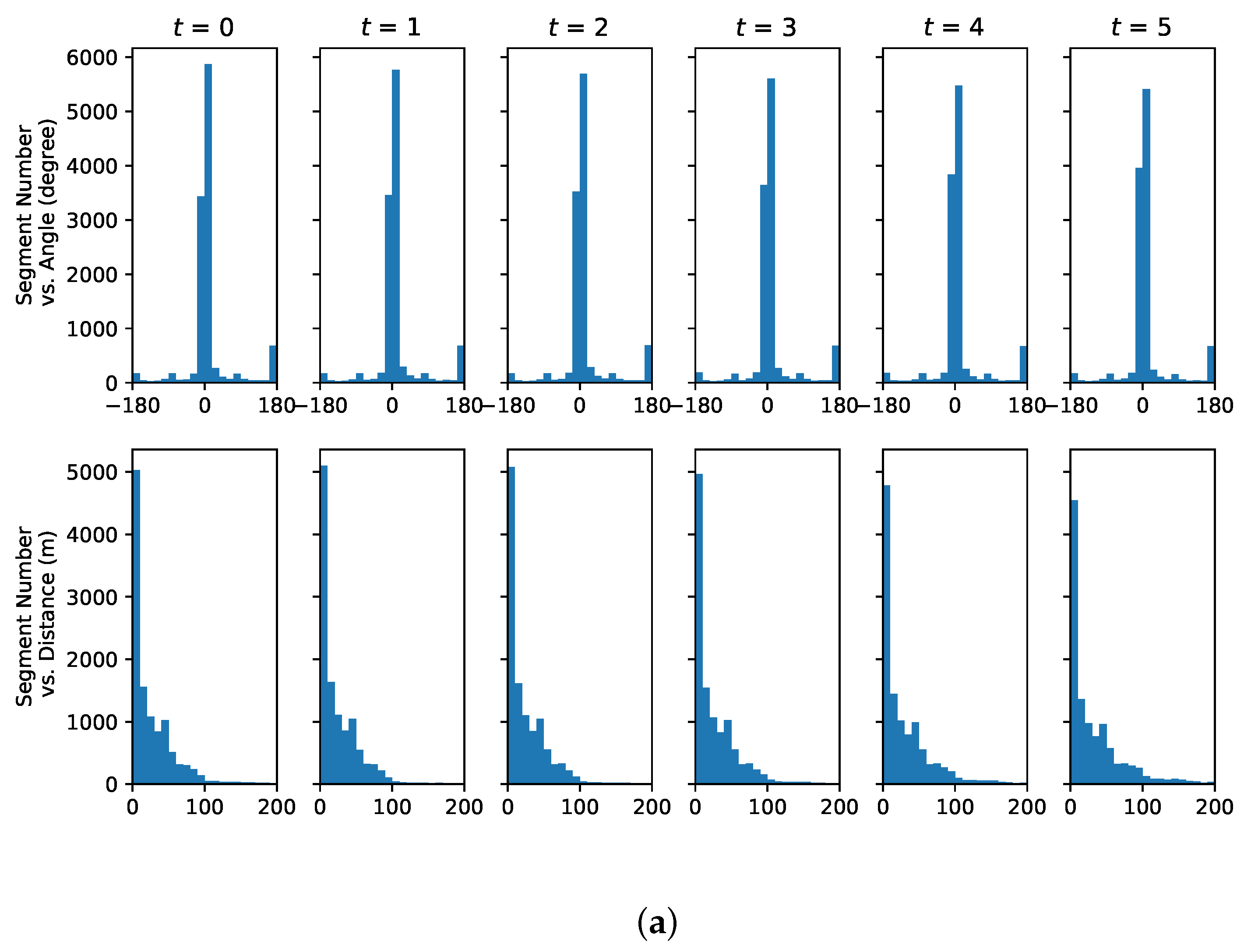
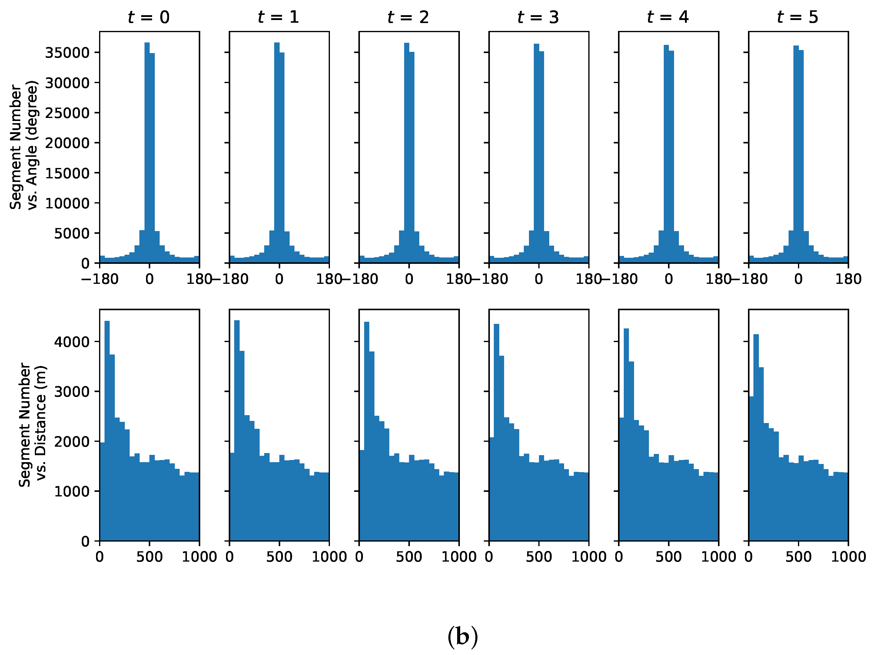
3.1. Data Preprocessing

Our approach considers two kinds of information obtained from animal trajectories. First, we use $d_t$ to denote the distance travelled at time period t. Second, we use ${\theta }_t$ to denote the change in motion direction. The positions of an animal at the beginning of time period $t-1$, t, and $t+1$ are $L_{t-1}$, $L_t$, and $L_{t+1}$, respectively, as recorded by a telemetry device. Thus, $d_t$ is the distance between $L_t$ and $L_{t+1}$, and ${\theta }_t$ is the difference between the direction from $L_{t-1}$ to $L_t$ and that from $L_t$ to $L_{t+1}$.

If we use $(L{o}_t,L{a}_t)$ to represent the longitude and latitude of an animal’s location at time t, we can calculate the distance between two consecutive locations ($(L{o}_t,L{a}_t)$ and $(L{o}_{t+1},L{a}_{t+1})$) using the haversine formula, and use it as the traveling distance $d_t$ at time t. To determine the animal’s turning angle, we first calculate the great circle angle relative to the North Pole for the trajectory from $(L{o}_{t-1},L{a}_{t-1})$ to $(L{o}_t,L{a}_t)$. We then calculate that angle for the trajectory from $(L{o}_t,L{a}_t)$ to $(L{o}_{t+1},L{a}_{t+1})$. By subtracting these two angles, we can obtain the turning angle ${\theta }_t$ of that animal at time t.

We use a sliding window of size T to obtain segments of a continuous trajectory, and input these segments into our model. As defined above, one input segment contains two sets of variables.

$$\begin{array}{c}\hfill \mathbf{d}=(d_1,d_2,\cdots ,d_T)\end{array}$$

(1)

$$\begin{array}{c}\hfill \mathbf{\theta }=({\theta }_1,{\theta }_2,\cdots ,{\theta }_T)\end{array}$$

(2)

Data augmentation is also widely used for deep learning and other classification methods to reduce limitations of datasets [11,25,26]. For example, if a certain class has a much larger sample size comparing to other classes, it can mislead a classifier to make biased predictions towards that large class. In our work, we balance the class size before training by randomly oversampling minority classes [25,26]. Namely, to create an oversampled class for class i, each data item in class i was sampled $\frac{N_{max}}{N_i}$ times, where $N_{max}$ is the the largest class size and $N_i$ is the class size of the ith class.

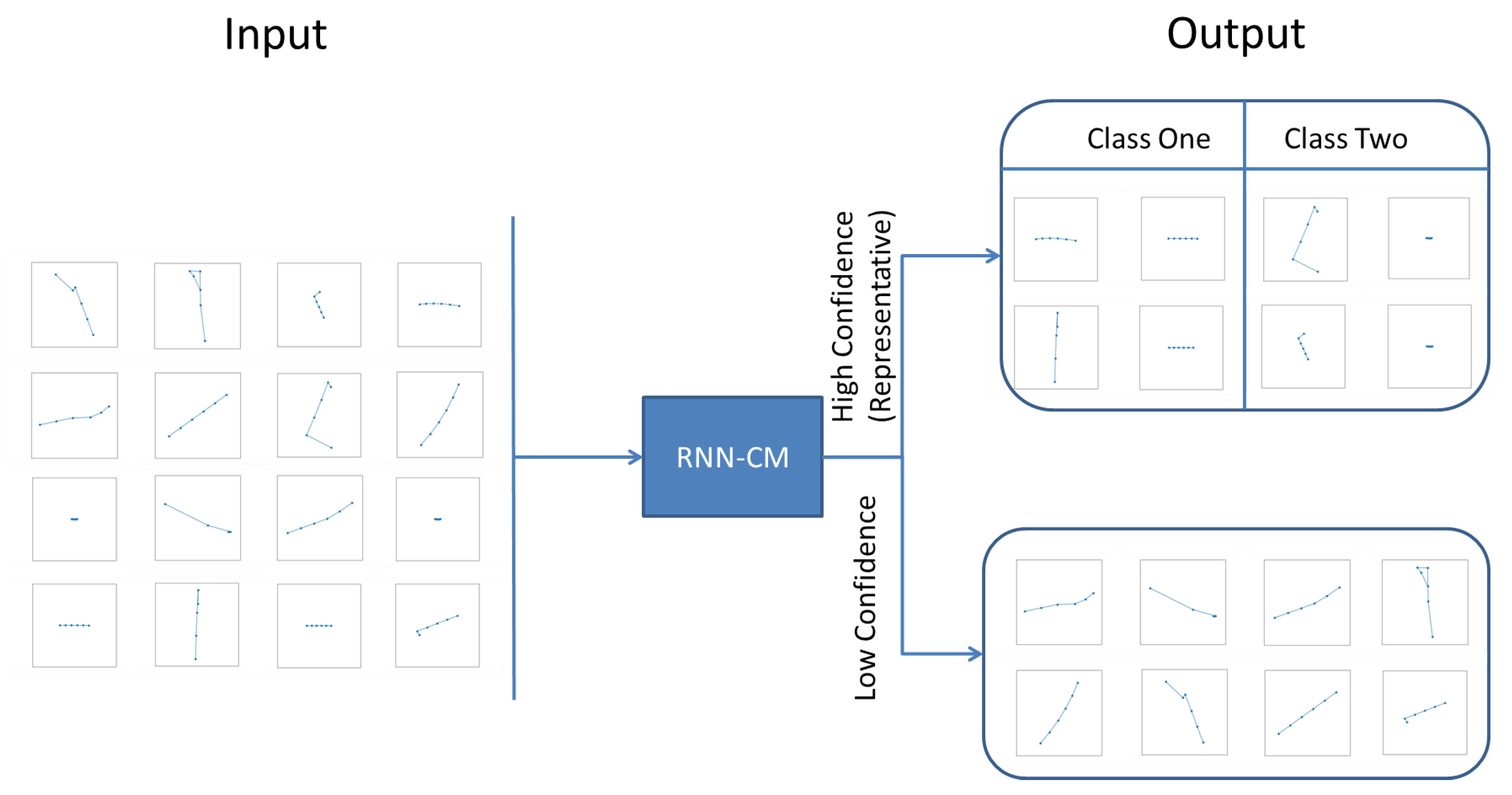
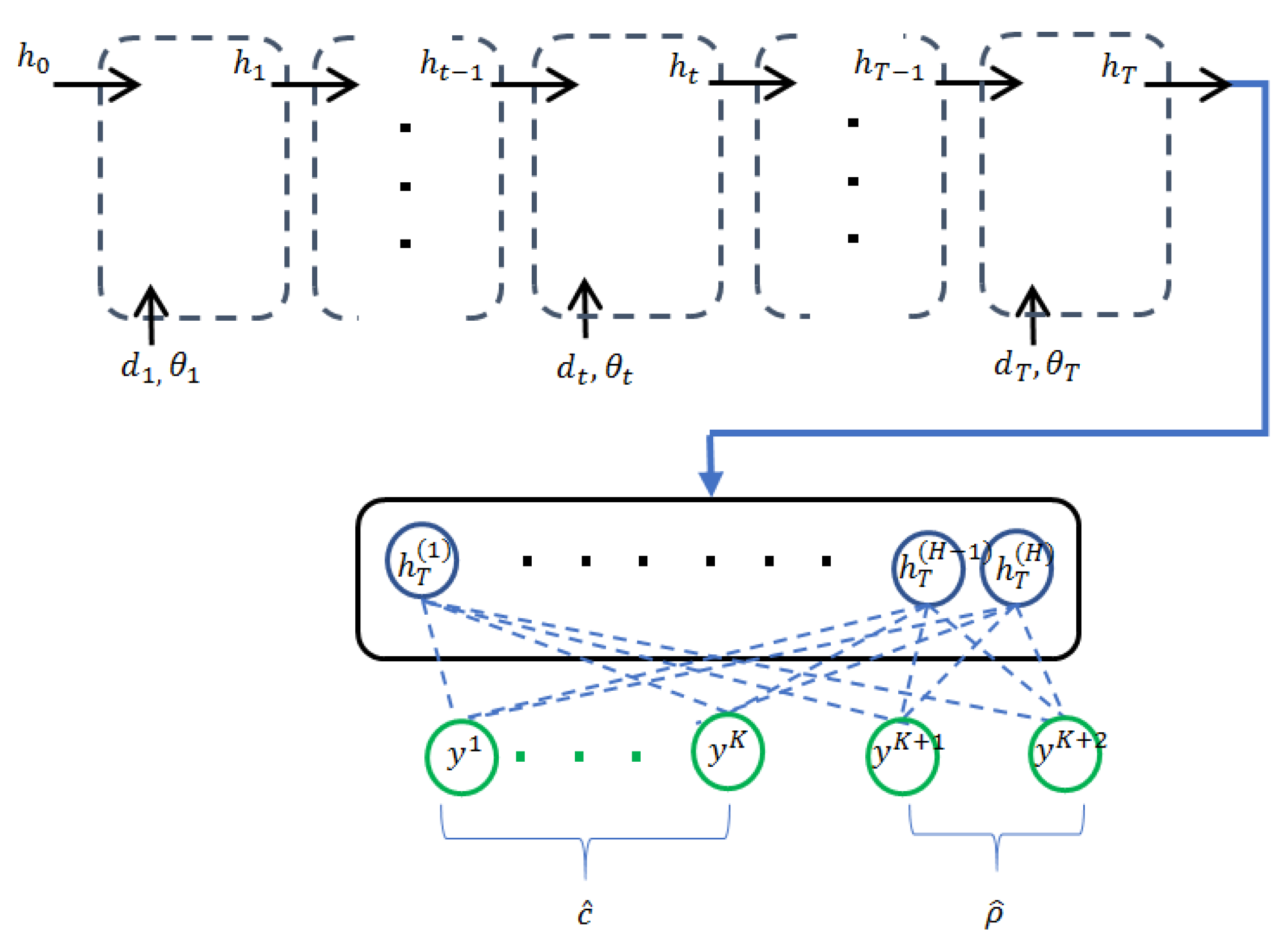
3.2. Recurrent Neural Networks with Confidence Measure

Some of their trajectory segments may differ significantly when the animals are from different age or gender groups. We therefore propose the problem that provided a trajectory segment, identifying relevant group identities for the owner of the segment. Without loss of generality, we consider that our animal dataset has K groups according to data labels.

Our neural network model is composed of two parts. The first part is an RNN that can extract features from the input trajectory segments. The second part includes two single-layer neural networks, each of which is fed by the output of the aforementioned RNN. These two single-layer networks are used for predicting group labels and for estimating the confidence of the predictions, respectively. Thus, the overall network is a recurrent neural network with a confidence measure.

For the first part, we use the long short-term memory (LSTM) network [27,28] as the basic element for analysis. An LSTM cell for time step t takes a tuple ($d_t$ and ${\theta }_t$) as the input. Each LSTM cell is in its basic form [27] except that the state variable $h_t$ is a vector [28]. In our model, we connect these LSTM cells in accordance with their represented time steps, so that variables at different time steps are not isolated:

$$\begin{array}{c}\hfill h_t=\mathbf{f}([d_t,{\theta }_t],h_{t-1}),\mathrm{for}t=1,2,\cdots ,T.\end{array}$$

(3)

where $h_0$ is initialized randomly.

In the second part, we use the hidden state of the last LSTM cell as the features for group prediction. If in total there are K groups, we define a binary vector c with length K as the ground-truth group indicator. Only one entry in c can be one and the index of that entry corresponds to the group label. We use vector $\widehat{c}$ of the same length to represent an estimator of c. With the value of the last hidden state $h_T$, we use a fully connected layer to compute the animal group estimator $\widehat{c}$ for each trajectory segment. We also use another fully connected layer to find the confidence $\rho$ of the estimator. The vector of $\rho$ is of length two. These two layers can be expressed by two equations as below:

$$\begin{array}{cc}\hfill \widehat{c}& =W_c{h}_T+b_c,\hfill \end{array}$$

(4)

$$\begin{array}{cc}\hfill \widehat{\rho }& =W_{\rho }{h}_T+b_{\rho },\hfill \end{array}$$

(5)

where $W_c\in {\mathbb{R}}^{K\times H}$ and $W_{\rho }\in {\mathbb{R}}^{2\times H}$ are weight matrices, and $b_c\in {\mathbb{R}}^{K\times 1}$ and $b_{\rho }\in {\mathbb{R}}^{2\times 1}$ are bias vectors. Without loss of generality, we consider the state vector $h_T$ as a column vector of size H.

An illustration of the network architecture is shown in Figure 2, in which the two fully connected networks for computing $\widehat{c}$ and $\widehat{\rho }$ can be considered as a single network for computing variable y. Variable $\widehat{c}$ and $\widehat{\rho }$ are then normalized respectively for the robustness of the approach.

Since only a scalar is needed as a confidence indicator, we use a softmax function, $h(·)$, to normalize $\widehat{\rho }$ and then take the leading entry as the indicator.

$$\begin{array}{cc}\hfill \tilde{\rho }& =h\left(\widehat{\rho }\right)\left[0\right]=\frac{e^{\widehat{\rho }\left[0\right]}}{{\sum }_{k=0}^1{e}^{\widehat{\rho }\left[k\right]}}.\hfill \end{array}$$

(6)

In practice, trajectory segments corresponding to certain behaviours (e.g., migration) may be quite similar for animals from different groups. In this case, classifiers are most likely to make incorrect or random predictions. We therefore consider these segments unpredictable. On the other hand, some trajectory segments associated with other behaviours may be quite different between different animal groups. The classifiers from these segments can therefore more readily predict the group membership of the animals from these segments, and we consider them as representative segments for the group. Our aim is to design a classifier that makes good predictions on predictable segments while ignoring unpredictable ones.

For this purpose, we introduce a new estimator $\tilde{c}$ by using a softmax function to incorporate the confidence variable with the previous estimator. The variable $\tilde{c}$ is also a vector, and each element of the vector is defined in Equation (7).

$$\begin{array}{c}\hfill \tilde{c}\left[j\right]=h\left(\widehat{c}\tilde{\rho }\right)\left[j\right]=\frac{e^{\widehat{c}\left[j\right]\tilde{\rho }}}{{\sum }_{k=1}^K{e}^{\widehat{c}\left[k\right]\tilde{\rho }}}.\end{array}$$

(7)

In this way, for predictable segments, the confidence is high (close to one) and $\tilde{c}$ is close to the output $\widehat{c}$ of the fully connected layer. For unpredictable segments, the confidence of the prediction is low (close to zero), so that the group identifier $\tilde{c}$ is neutralized. Here the term “neutralized” means that all the entries of the vector have similar values such that each segment has a similar probability of belonging to any animal group.

To minimize the difference between the estimator, $\tilde{c}$, and the ground truth, c, we define the cost function as the cross entropy of these two vectors as below:

$$\begin{array}{c}\hfill G(\tilde{c},c)=-\sum _{j=0}^{K-1}c\left[j\right]log\left(\tilde{c}\left[j\right]\right)+\lambda \sum _{j=0}^{K-1}\tilde{\rho }\left[j\right],\end{array}$$

(8)

where the last term is an additional regularization on the confidence scores, and the hyperparameter, $\lambda$, is the weight of the regularization. We minimize the cost function during training to obtain optimal $W_c$, $b_c$, $W_{\rho }$, and $b_{\rho }$.

For classification, we can feed the trajectory segments into Equation (3) and after a series of computations, we can obtain the estimated group label $\tilde{c}$ and the confidence of the estimation $\tilde{\rho }$ from Equation (7) and Equation (6) respectively. To find the representative segments, we can apply classification algorithms to estimate which segments can best represent the corresponding animal’s group identity. In our approach, we use $\tilde{\rho }$ as the confidence score. We measure the accuracy by computing the fraction of trajectory segments with y equal to $\tilde{y}$, where

$$\begin{array}{cc}\hfill \tilde{y}& =arg\underset{i}{max}\tilde{c}\left[i\right]\hfill \end{array}$$

(9)

$$\begin{array}{cc}\hfill y& =arg\underset{i}{max}c\left[i\right].\hfill \end{array}$$

(10)

In practice, if the accuracy of the high-confidence segments is relatively low, we can raise $\lambda$ to further restrict the confidence of the mistaken predictions. When the accuracy of the high-confidence segments is relatively high, the high confidence segments are representative segments of corresponding groups as predicted. We use $\lambda =0$ by default.

3.3. Multi-Scale Recurrent Neural Networks

The approach above can “translate” the pattern of a T-hour segment into a group label. In addition, while keeping the T-hour information, we can also emphasize the last few hours (e.g., $T/2$) for the “translation”.

To achieve this, we can build another LSTM network by feeding less data (e.g., $T/2<t\le T$) into Equation (3), and obtain the final state at $t=T$ (denoted as $h_T^S$). Then, we concatenate $h_T$ with $h_T^S$, and correspondingly increase the number of columns for $W_c$ and $W_{\rho }$ in Equation (4) correspondingly. With other variables unaffected, we can minimize a similar cost function during the training.

Adding additional scales is possible by building additional separate LSTM networks and concatenating their last hidden states with $h_T$. Then, only the size of the corresponding variables is changed, but the whole framework can still be the same.

We use Adam optimizer in Tensorflow [29] for neural network optimization.

3.4. Data Set

We use a dataset that includes trajectories of 489,391 hours from 111 southern elephant seals (Mirounga leonina, 32 females and 79 males), and their positions obtained from Argos platform transmitter terminals. All procedures to obtain the data were approved by the respective ethics committees and licensing bodies including, the Australian Antarctic Animal Ethics Committee (ASAC 2265, AAS 2794, AAS 4329), the Tasmanian Parks and Wildlife Service, the University of California, Santa Cruz and the Programa Antártico Brasileiro. The procedures were carried out in accordance with current guidelines and regulations.

For each trajectory, we use a T-hour sliding window to extract length-T trajectory segments. We use tr-T to represent the set of segments. The majority of the female seals in our dataset were adult seals (two were juveniles) and all of the male seals were juveniles or subadults. We therefore considered representative patterns from gender groups. We randomly selected 80% of the individuals in each group and used their segments for training. We selected the remaining 20% of the seals and extracted their segments for testing. We set $T=6$ in this experiment.

4. Results

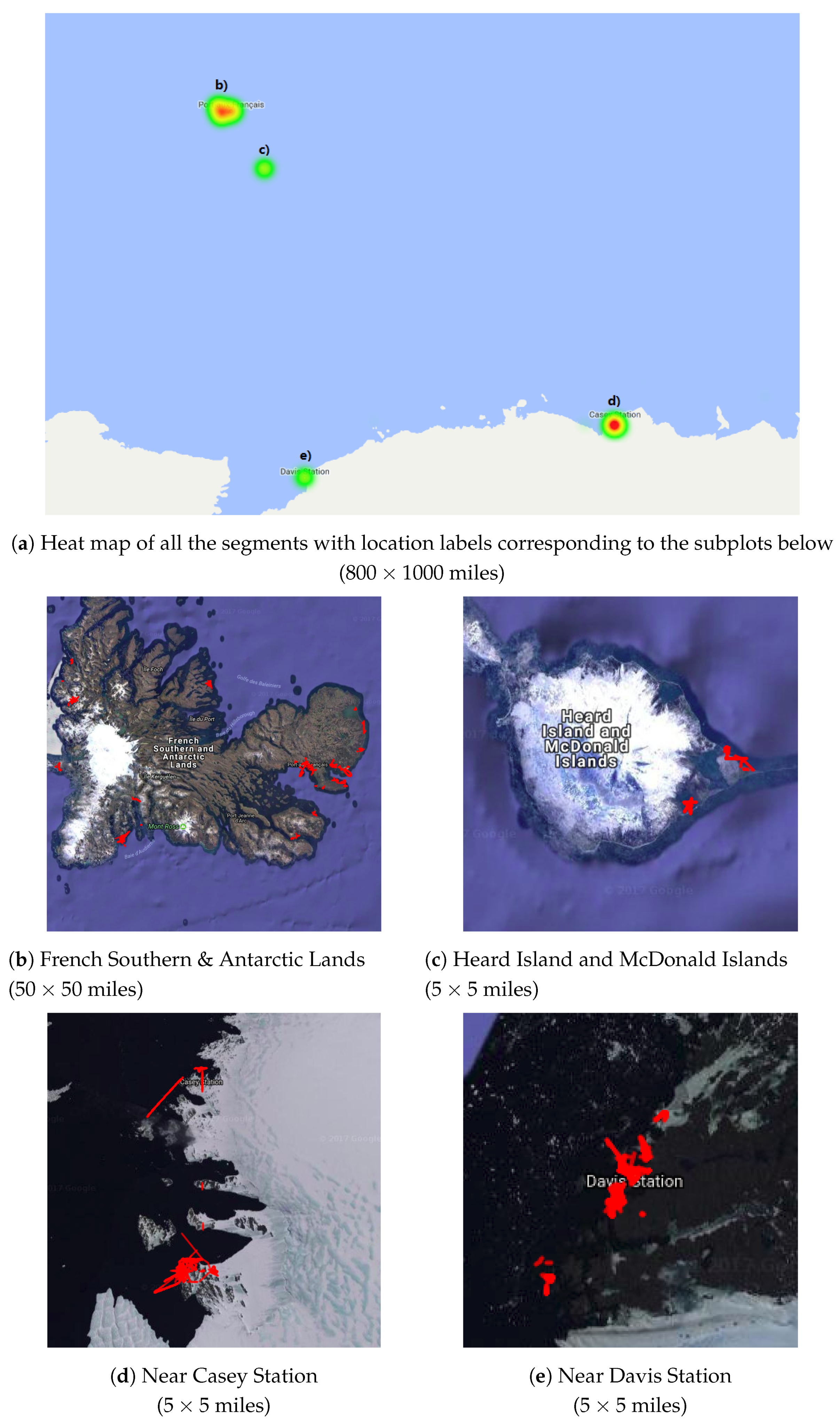
4.1. Representative Trajectory Segments

RNN-CM allowed us to identify segments with the highest confidence scores. To propose representative segments for a specific group, we predict animal group identities for each segment and estimate confidence scores for the predictions. Segments with high confidence scores were deemed to be representative ones. We call such segments Representative Segments (RES). They are unique to a specific group (here, male seals), whereas other segments are Common Segments (COS) whose patterns are shared by different animal groups (here, males and females, and thus, $K=2$). The RES and COS patterns are fundamentally different. To investigate the characteristics of RES, we focus our discussion on the segments with top-10% confidence scores obtained by RNN-CM. For segments in RES and COS, histograms with respect to distance $d_t$ (in meters) and with respect to turning angle ${\theta }_t$ (in degrees) for $t=0,1,2,\cdots ,T-1$ are presented by the first and the second rows of each subplot in Figure 3. As shown by the histograms, segments in RES are generally short distance movements and are more likely to follow an unbalanced pattern with a slightly right turn or even a turn in almost the opposite direction. Given that RES capture the movements of male seals, this could be a unique pattern for the males for our data set.

4.2. Effectiveness of the Proposed RNN-CM Model

To evaluate the effectiveness of our RNN-CM model, we compared the accuracy of classification based on the proposed representative segments among different algorithms, including two traditional classification methods, namely, Linear Support Vector Machine (Linear SVM) [30,31] and Random Forest methods [32]. These two traditional algorithms have been widely used for data classification [33]. We first trained each algorithm and then used it to identify representative segments with confidence scores from the same given dataset. In Linear SVM, the confidence score of a datum is the signed distance of that sample to the hyperplane. In Random Forest, there are multiple decision trees and the confidence score is the mean predicted class probability of the trees in the forest. Then, we compared their accuracy, which is measured as the ratio of correct classifications to all classifications.

The results in

Table 1. The accuracy of classification based on the proposed representative segments (male segment fraction of all the high confidence segments) as determined by different algorithms on segments extracted from a trajectory using a T-hour ($T=6$) sliding window.

Confidence Level	Top 10%	Top 20%	Top 30%	All
RNN-CM	91.1% [100%]	85.2% [100%]	79.4% [99.5%]	54.6% [59.0%]
Random Forest	83.5% [99.5%]	78.4% [94.4%]	72.1% [85.8%]	57.0% [65.4%]
Linear SVM	85.6% [100.0%]	78.8% [100.0%]	75.2% [100.0%]	49.8% [48.3%]

reveal that none of the algorithms perform well when the whole dataset is taken into account, regardless of the confidence scores (the “All” column). This is because seals in different groups can have lots of similar segments as they belong to the same species, and thus, it is difficult for a classification algorithm to identify the labels of these similar segments in high accuracy. In this case, classifiers perform as random estimators and the accuracy is around 50% for the two class classification.

If we raise the confidence threshold as shown from right to left, i.e., if we consider only the predictions with the top $X\%$$(X=10,20,30)$ confidence scores by each algorithm, the accuracy is increasing because classifiers gradually ignore low confidence estimations and concentrate on high confidence ones. In such a case, the accuracy of our approach is significantly higher than that of the other approaches. This is because our approach with deep learning architecture can better describe latent patterns in the data than other approaches, so that the prediction based on such patterns can be more accurate. In addition, our confidence measure is integrated together with the classifier during training, so that it can be better optimized than training the classifier only. We also present the male seal segment fraction of the top $X\%$$(X=10,20,30)$ confidence segments, as indicated in brackets of Table 1. These fractions indicate that most of the representative segments belong to males.

In short, if some trajectory patterns are shared by different animal groups, a classification algorithm can be confused and cannot make correct group predictions, and consequently gives low confidence scores for such patterns. On the other hand, trajectory segments that can earn high confidence scores are generally patterns that are unique to the corresponding animal group. Thus, our algorithm can identify group-specific patterns more accurately.

In the experiment, the training segments and the testing segments are from different seals. The consistency of the testing results and the training objectives also indicates that animals in the same group can share some patterns of trajectory segments.

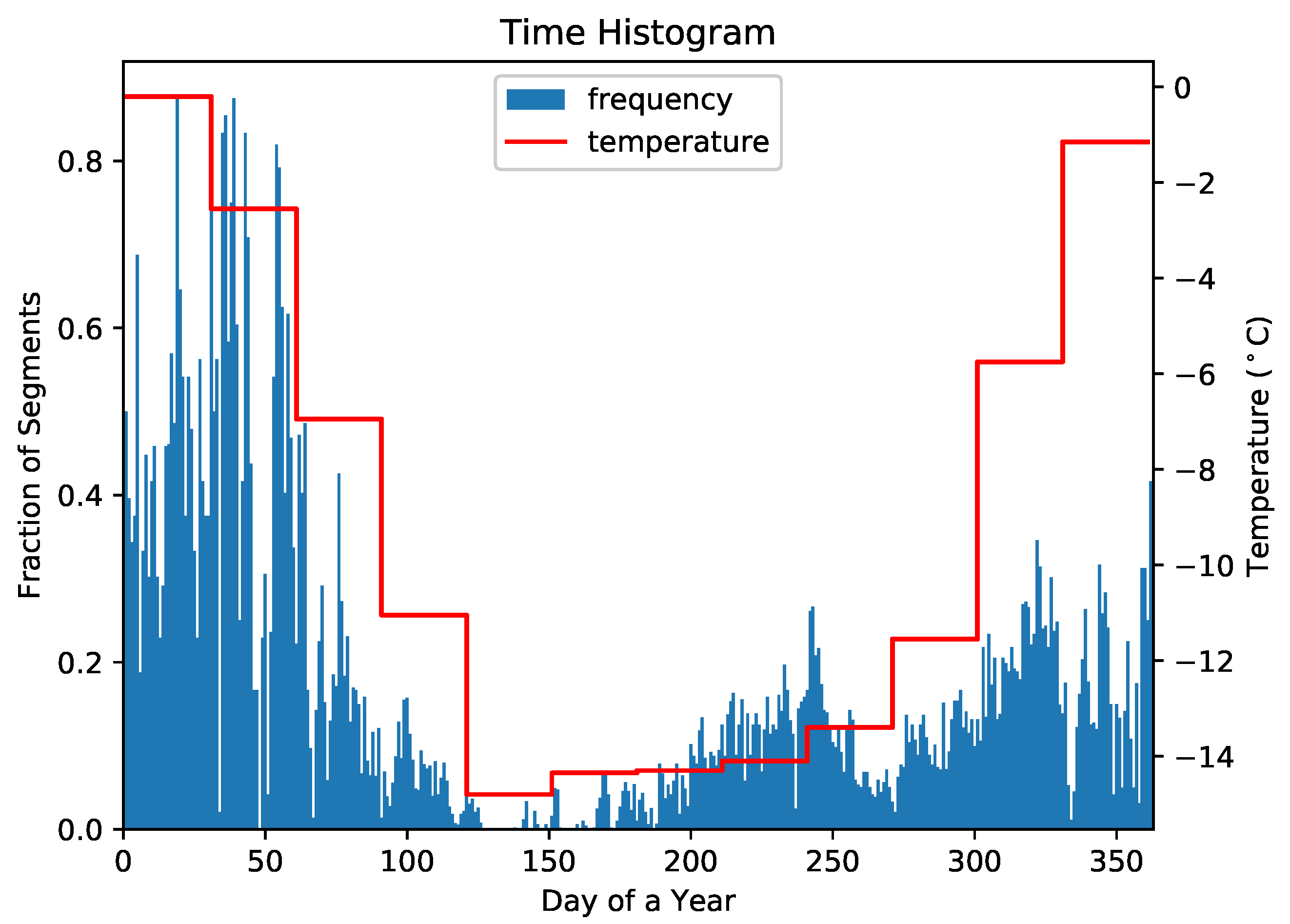
4.3. Understanding Representative Trajectory Segments

To understand the representative trajectory segments, we examined the locations where the representative segments took place. Figure 4a presents a heat map that shows the locations of the representative segments, where red indicates the most concentrated regions and green indicates the least concentrated regions. As the heat map shows, most segments are near the coastlines of Antarctica and nearby islands. The enlarged satellite images from Google Maps in Figure 4b–e show the segments as red spots. These enlarged images show that the segments are mostly on land and sometimes in water. In addition, the locations on land are concentrated. The seals are likely to go to the same place on the land after returning from various trips. The red spots on land clearly indicate the seals’ colonies.

The histogram in Figure 5 shows the relationship between time of the year and RES, i.e., illustrating the fraction of RES for each day of the year. We also plot the monthly average temperature at the Casey Station, which is representative of the relative temperature in the region over time. From this figure, we can see that RES are less frequent in May (autumn) when seals are at sea, and more frequent in January until March, tying in with the period of the moult when seals are spending time ashore or very close to shore.

As suggested by previous research, coastal polynyas are important habitats for juvenile male seals [34]. In this experiment, the representative trajectory segments usually took place near coastal land and belong to male seals. Thus, such segments could be related to their habitat activities. In addition, these recurring segment patterns are likely to be associated with the memory system of these seals, which is also in accordance with previous research [35]. Specifically, because RES and temperature are positively correlated, and RES contain lots of short near coastline trips, they appear to be related to periods when the young male seals are ashore for molting or resting. The transmitters were attached near the end of the molting period when the seals’ old fur has been shed and the new fur has largely regrown. Some juveniles/sub-adult seals also come ashore between April and August to rest.

4.4. Conclusions

Marine animal movement analysis provides important information for behavioural ecology. Traditional approaches such as state-space models focus on identifying the purposes of trajectory segments, but to date adding covariates including group characteristics like sex have been difficult. In this work, we proposed an approach to identifying trajectory segments that are representative of the movements of marine animal subgroups. Our method contributes to understanding marine animal habitats and activities, especially when group classification, such as by sex or age, is unknown or difficult to determine morphologically.

References

1. Block, B.A.; Jonsen, I.D.; Jorgensen, S.J.; Winship, A.J.; Shaffer, S.A.; Bograd, S.J.; Hazen, E.L.; Foley, D.G.; Breed, G.; Harrison, A.L.; et al. Tracking apex marine predator movements in a dynamic ocean. Nature 2011, 475, 86–90. [Google Scholar] [CrossRef] [PubMed]
2. Burton, A.; Groenewegen, D.; Love, C.; Treloar, A.; Wilkinson, R. Making research data available in Australia. IEEE Intell. Syst. 2012, 27, 40–43. [Google Scholar] [CrossRef]
3. Giuggioli, L.; Bartumeus, F. Animal movement, search strategies and behavioural ecology: A cross-disciplinary way forward. J. Anim. Ecol. 2010, 79, 906–909. [Google Scholar] [CrossRef] [PubMed]
4. Hays, G.C.; Ferreira, L.C.; Sequeira, A.M.; Meekan, M.G.; Duarte, C.M.; Bailey, H.; Bailleul, F.; Bowen, W.D.; Caley, M.J.; Costa, D.P.; et al. Key questions in marine megafauna movement ecology. Trends Ecol. Evol. 2016, 31, 463–475. [Google Scholar] [CrossRef] [PubMed]
5. Kays, R.; Crofoot, M.C.; Jetz, W.; Wikelski, M. Terrestrial animal tracking as an eye on life and planet. Science 2015, 348. [Google Scholar] [CrossRef] [PubMed]
6. Cotté, C.; d’Ovidio, F.; Dragon, A.C.; Guinet, C.; Lévy, M. Flexible preference of southern elephant seals for distinct mesoscale features within the Antarctic Circumpolar Current. Prog. Oceanogr. 2015, 131, 46–58. [Google Scholar] [CrossRef] [Green Version]
7. Gaspar, P.; Georges, J.Y.; Fossette, S.; Lenoble, A.; Ferraroli, S.; Le Maho, Y. Marine animal behaviour: Neglecting ocean currents can lead us up the wrong track. Proc. R. Soc. Lond. B Biol. Sci. 2006, 273, 2697–2702. [Google Scholar] [CrossRef]
8. Campagna, C.; Piola, A.R.; Marin, M.R.; Lewis, M.; Fernández, T. Southern elephant seal trajectories, fronts and eddies in the Brazil/Malvinas Confluence. Deep Sea Res. Part I Oceanogr. Res. Pap. 2006, 53, 1907–1924. [Google Scholar] [CrossRef]
9. LeCun, Y.; Bengio, Y.; Hinton, G. Deep learning. Nature 2015, 521, 436. [Google Scholar] [CrossRef]
10. Chen, Y.; Lin, Z.; Zhao, X.; Wang, G.; Gu, Y. Deep learning-based classification of hyperspectral data. IEEE J. Sel. Top. Appl. Earth Obs. Remote Sens. 2014, 7, 2094–2107. [Google Scholar] [CrossRef]
11. Krizhevsky, A.; Sutskever, I.; Hinton, G.E. Imagenet classification with deep convolutional neural networks. Adv. Neural Inf. Proc. Syst. 2012, 1097–1105. [Google Scholar] [CrossRef]
12. Cai, Z.; Vasconcelos, N. Cascade r-cnn: Delving into high quality object detection. In Proceedings of the IEEE Conference on Computer Vision and Pattern Recognition, Salt Lake City, UT, USA, 18–22 June 2018; pp. 6154–6162. [Google Scholar]
13. Chambon, S.; Galtier, M.N.; Arnal, P.J.; Wainrib, G.; Gramfort, A. A deep learning architecture for temporal sleep stage classification using multivariate and multimodal time series. IEEE Trans. Neural Syst. Rehabil. Eng. 2018, 26, 758–769. [Google Scholar] [CrossRef] [PubMed]
14. Pedersen, M.; Bruslund Haurum, J.; Gade, R.; Moeslund, T.B. Detection of Marine Animals in a New Underwater Dataset with Varying Visibility. In Proceedings of the IEEE Conference on Computer Vision and Pattern Recognition Workshops, Long Beach, CA, USA, 15–21 June 2019; pp. 18–26. [Google Scholar]
15. Sun, R.; Giles, C.L. Sequence learning: From recognition and prediction to sequential decision making. IEEE Intell. Syst. 2001, 16, 67–70. [Google Scholar] [CrossRef]
16. Grossman, G.D.; Nickerson, D.M.; Freeman, M.C. Principal component analyses of assemblage structure data: Utility of tests based on eigenvalues. Ecology 1991, 72, 341–347. [Google Scholar] [CrossRef]
17. Smouse, P.E.; Focardi, S.; Moorcroft, P.R.; Kie, J.G.; Forester, J.D.; Morales, J.M. Stochastic modelling of animal movement. Philos. Trans. R. Soc. Lond. B: Biol. Sci. 2010, 365, 2201–2211. [Google Scholar] [CrossRef] [PubMed] [Green Version]
18. Patterson, T.A.; Thomas, L.; Wilcox, C.; Ovaskainen, O.; Matthiopoulos, J. State-space models of individual animal movement. Trends Ecol. Evol. 2008, 23, 87–94. [Google Scholar] [CrossRef] [PubMed]
19. Langrock, R.; King, R.; Matthiopoulos, J.; Thomas, L.; Fortin, D.; Morales, J.M. Flexible and practical modeling of animal telemetry data: hidden Markov models and extensions. Ecology 2012, 93, 2336–2342. [Google Scholar] [CrossRef] [PubMed]
20. Dalziel, B.D.; Morales, J.M.; Fryxell, J.M. Fitting probability distributions to animal movement trajectories: using artificial neural networks to link distance, resources, and memory. Am. Nat. 2008, 172, 248–258. [Google Scholar] [CrossRef] [PubMed]
21. Wu, F.; Lei, T.K.H.; Li, Z.; Han, J. Movemine 2.0: Mining object relationships from movement data. Proc. VLDB Endow. 2014, 7, 1613–1616. [Google Scholar] [CrossRef]
22. Yuan, G.; Sun, P.; Zhao, J.; Li, D.; Wang, C. A review of moving object trajectory clustering algorithms. Artif. Intell. Rev. 2017, 47, 123–144. [Google Scholar] [CrossRef]
23. Shamoun-Baranes, J.; Dokter, A.M.; van Gasteren, H.; van Loon, E.E.; Leijnse, H.; Bouten, W. Birds flee en mass from New Year’s Eve fireworks. Behav. Ecol. 2011, 22, 1173–1177. [Google Scholar] [CrossRef] [PubMed]
24. Zheng, Y. Trajectory data mining: an overview. ACM Trans. Intell. Syst. Technol. 2015, 6, 29. [Google Scholar] [CrossRef]
25. More, A. Survey of resampling techniques for improving classification performance in unbalanced datasets. arXiv 2016, arXiv:1608.06048. [Google Scholar]
26. Crone, S.F.; Finlay, S. Instance sampling in credit scoring: An empirical study of sample size and balancing. Int. J. Forecast. 2012, 28, 224–238. [Google Scholar] [CrossRef]
27. Gers, F.A.; Schmidhuber, J.; Cummins, F. Learning to Forget: Continual Prediction with LSTM. Neural Comput. 2000, 12, 2451–2471. [Google Scholar] [CrossRef] [PubMed]
28. Zaremba, W.; Sutskever, I.; Vinyals, O. Recurrent neural network regularization. arXiv 2014, arXiv:1409.2329. [Google Scholar]
29. Abadi, M.; Agarwal, A.; Barham, P.; Brevdo, E.; Chen, Z.; Citro, C.; Corrado, G.S.; Davis, A.; Dean, J.; Devin, M.; et al. TensorFlow: Large-Scale Machine Learning on Heterogeneous Systems. 2015. Available online: www.tensorflow.org (accessed on 1 July 2019).
30. Fan, R.E.; Chang, K.W.; Hsieh, C.J.; Wang, X.R.; Lin, C.J. LIBLINEAR: A library for large linear classification. J. Mach. Learn. Res. 2008, 9, 1871–1874. [Google Scholar]
31. Hsia, C.Y.; Zhu, Y.; Lin, C.J. A study on trust region update rules in Newton methods for large-scale linear classification. In Proceedings of the Asian Conference on Machine Learning (ACML), Seoul, Korea, 15–17 November 2017. [Google Scholar]
32. Breiman, L. Random forests. Mach. Learn. 2001, 45, 5–32. [Google Scholar] [CrossRef]
33. Zhang, C.; Liu, C.; Zhang, X.; Almpanidis, G. An up-to-date comparison of state-of-the-art classification algorithms. Exp. Syst. Appl. 2017, 82, 128–150. [Google Scholar] [CrossRef]
34. Labrousse, S.; Williams, G.; Tamura, T.; Bestley, S.; Sallée, J.B.; Fraser, A.D.; Sumner, M.; Roquet, F.; Heerah, K.; Picard, B.; et al. Coastal polynyas: Winter oases for subadult southern elephant seals in East Antarctica. Sci. Rep. 2018, 8, 3183. [Google Scholar] [CrossRef]
35. Rodríguez, J.P.; Fernández-Gracia, J.; Thums, M.; Hindell, M.A.; Sequeira, A.M.; Meekan, M.G.; Costa, D.P.; Guinet, C.; Harcourt, R.G.; McMahon, C.R.; et al. Big data analyses reveal patterns and drivers of the movements of southern elephant seals. Sci. Rep. 2017, 7, 112. [Google Scholar] [CrossRef] [PubMed]
Figure 1. The recurrent neural network with confidence measure (RNN-CM) process with sample inputs. Left side contains the input segments from marine animals with multiple age or gender groups, which are processed by RNN-CM. The processed segments can be divided into high and low confidence ones. The patterns of low confidence segments are shared by different animal groups, and thus, RNN-CM has low confidence in identifying which group they are extracted from. High confidence segments can be further divided according to animal age or gender groups, with relatively high confidence.
Applsci 09 02935 g001
Figure 2. The network architecture of the recurrent neural network with confidence measure (RNN-CM). The boxes in the first row are long short-term memory (LSTM) cells, and the hidden state of the last cell is fed to a fully connected neural network. The superscripts are element indices of vectors.
Applsci 09 02935 g002
Figure 3. Histograms of distances and angles for trajectory segments with different confidences. Representative segments are those with high confidences, while common segments are those with low confidences. t= 0,1,2,3,4,5 are time units of one segment. (a) Representative segments; (b) Common segments.
Applsci 09 02935 g003aApplsci 09 02935 g003b
Figure 4. Locations of the representative trajectory segments (Approximate area size), https://www.google.com/maps Map data ©2018 Imagery ©2018 NASA ©2018 Google Terms of Use.
Applsci 09 02935 g004
Figure 5. Fraction of Representative Segments and Average Temperature Over Different Time of Year.
Applsci 09 02935 g005