Article

FEM-Based Compression Fracture Risk Assessment in Osteoporotic Lumbar Vertebra L1

by
Algirdas Maknickas
1,*,
Vidmantas Alekna
2,
Oleg Ardatov
1,
Olga Chabarova
3,
Darius Zabulionis
4,
Marija Tamulaitienė
2 and
Rimantas Kačianauskas
1,4
1
Institute of Mechanics, Vilnius Gediminas Technical University, 03224 Vilnius, Lithuania
2
Faculty of Medicine, Vilnius University, 03101 Vilnius, Lithuania
3
Department of Applied Mechanics, Vilnius Gediminas Technical University, 10223 Vilnius, Lithuania
4
Department of Information Systems, Vilnius Gediminas Technical University, 10223 Vilnius, Lithuania
*
Author to whom correspondence should be addressed.
Appl. Sci. 2019, 9(15), 3013; https://doi.org/10.3390/app9153013
Submission received: 27 June 2019 / Revised: 19 July 2019 / Accepted: 24 July 2019 / Published: 26 July 2019
(This article belongs to the Special Issue Biomaterials for Bone Tissue Engineering)

Abstract

:
This paper presents a finite element method (FEM)-based fracture risk assessment in patient-specific osteoporotic lumbar vertebra L1. The influence of osteoporosis is defined by variation of parameters such as thickness of the cortical shell, the bone volume–total volume ratio (BV/TV), and the trabecular bone score (TBS). The mechanical behaviour of bone is defined using the Ramberg–Osgood material model. This study involves the static and nonlinear dynamic calculations of von Mises stresses and follows statistical processing of the obtained results in order to develop the patient-specific vertebra reliability. In addition, different scenarios of parameters show that the reliability of the proposed model of human vertebra highly decreases with low levels of BV/TV and is critical due to the thinner cortical bone, suggesting high trauma risk by reason of osteoporosis.

Graphical Abstract

1. Introduction

Spinal bones can be affected by several diseases, but spinal brittleness is mainly caused by osteoporosis. Due to the importance of studying this disease and its consequences, various social and medical aspects of osteoporosis have been investigated all over the world [1,2,3,4]. A comprehensive discussion of the role of computational biomechanical modeling is presented in a review article by Doblare et al. [5]. The paper emphasized numerical modeling as the main directions for future research. The adequacy of the modeling of finite elements strongly depends on the selection of the mechanical properties, the geometrical form of the numerical model, and mesh making possibilities.
With regard to considerable difficulties in the assignment of the anatomical geometry to the model, most researches are focused on simplifications. Some developments are restrained to small fragments of the vertebra [6,7], but most studies concerning the vertebral body in isolation [8,9,10,11] also use a simplified form, excluding the posterior elements [12,13].
A two-scale modeling approach was proposed in a series of papers where the macroscopic defining behavior is defined by the influence of the microstructure. For example, the work of McDonald et al. used a microscopic lattice network [12]. A similar approach was applied by Reference [14]. In contrast, a more comprehensive method of modeling was used in Reference [15] where the porous trabecular cell in the cancellous bone is considered as three-dimensional solid.
To determine the level of stress and bone strength, classical criteria for fluidity at the continuum level are often applied. Thus, the von Mises yield criterion is the most frequently used [11] criterion used for the trabecular bone of a vertebra, but a tissue-dependent orthotropic yield criterion Tsai–Wu [16] was proposed also.
In most cases, studies were perfomed by using static loads, while the number of investigations with dynamic loads are rather limited [13,17]. Also, the computational biomechanics can provide the ability to assess fracture risk and can serve as a useful diagnostic tool for analysing the state of osteoporotic bones. One of the most effective modern indicators used to verify vertebral fragility is the the trabecular bone score (TBS). This method involves the measurment of gray level texture, which shows the average state of trabecular bone microarchitecture [18], closely related to the ratio volume–total bone volume (BV/TV) [19]. Although TBS is a rough estimate of the strength properties of bone tissue, it can also be provided to study bone fragility and predict bone fractures.
There are several developed methods which employ bone mineral density (BMD) to predict the long-term fracture risk. BMD is usually assessed by dual-energy X-ray absorptiometry (DXA), and some studies have shown that a decrease of BMD is bonded with a higher risk for future fracture [20,21,22]. In addition, modern techniques of medical diagnostics also dispose computer-based algorithms, such as FRAX [23], which calculate fracture probability from clinical risk factors, such as age and body mass index(BMI), and dichotomized risk factors comprising prior fragility fracture, parental history of hip fracture, currently smoking tobacco, long-term oral glucocorticoid use, rheumatoid arthritis, other causes of secondary osteoporosis, and alcohol consumption [24]. In contrast, these methods do not verify the complicated relationship between the important parameters such as BV/TV, the thickness of the cortical shell, and the external load. The finite element method (FEM)-based continuum models can supply the additional patient-specific data to define the risk of fracture by additionally applying the reliability theory.
One of the aims of present work is numerical investigation of the osteoportic affect on strength properties of the proposed vertebrae model including the time-dependent load. The evaluation results might be useful for the medical diagnostics of the osteoporosis and for verifying the strength properties of the bone tissue of the patient. The main aim of this study is proposing the structural mechanics-based method of calculating fracture risk based on statistically processed results obtained by the numerical investigation of strength properties of the lumbar vertebral L1 body with various grades of osteoporotic degradation.

2. Methods and Materials

2.1. Problem Formulation

In order to model bone tissue as elastoplastic three-dimensional solid, the Ramberg–Osgood stress–strain equation was applied [25]:
ε = σ E 0 ε ˙ d + α σ K n ε ˙ b
where E 0 is the modulus of elasticity, K is the strain hardening coefficient, n is the strain-hardening exponent, and α is the yield offset, where ε ˙ = 1 equality was used. According to research [25], the loading rate of cortical bone influences the behaviour of the stress–strain relation. Therefore, our model of risk evaluation should be treated as the upper risk limit for load rates, which do not exceed rates of ε ˙ 1 .
In this work, the von Mises–Hencky criterion is chosen to predict the fracture of the model. It is defined in Equation (2): There, σ 1 , σ 2 and σ 3 are the maximum, intermediate and minimum principal stresses. σ Y presents yield stress (40 MPa) [26].
σ 1 σ 2 2 + σ 2 σ 3 2 + σ 3 σ 1 2 2 = σ Y
In the case of nonlinear analysis, the equilibrium equations are presented at time step t + Δ t :
M t + Δ t U ( i ) + C t + Δ t U ( i ) + t + Δ t K ( i ) t + Δ t Δ U ( i ) = t + Δ t R t + Δ t F ( i 1 )
where M is the mass matrix, C is the damping matrix, t + Δ t K ( i ) is the stiffness matrix, t + Δ t R is the vector of nodal loads, t + | d e l t a t F ( i 1 ) is the vector of nodal forces in case of iteration iteration ( i 1 ) , t + Δ t Δ U ( i ) is the vector nodal displacements while the iteration is ( i ) , t + Δ t U ( i ) is the vector of total velocities while the iteration is ( i ) , and M t + Δ t U ( i ) is the vector of total accelerations while the iterations is ( i ) . Using an implicit time integration Newmark–Beta scheme and employing Newton’s iterative method, the presented equations are cast in the following form:
t + Δ t K ( i ) t + Δ t Δ U ( i ) = t + Δ t R
where t + Δ t R ( i ) is the effective load vector and t + Δ t K ( i ) is the effective stiffness matrix. The three-dimensional static and dynamic analyses were performed using Abaqus (c) [27] software.

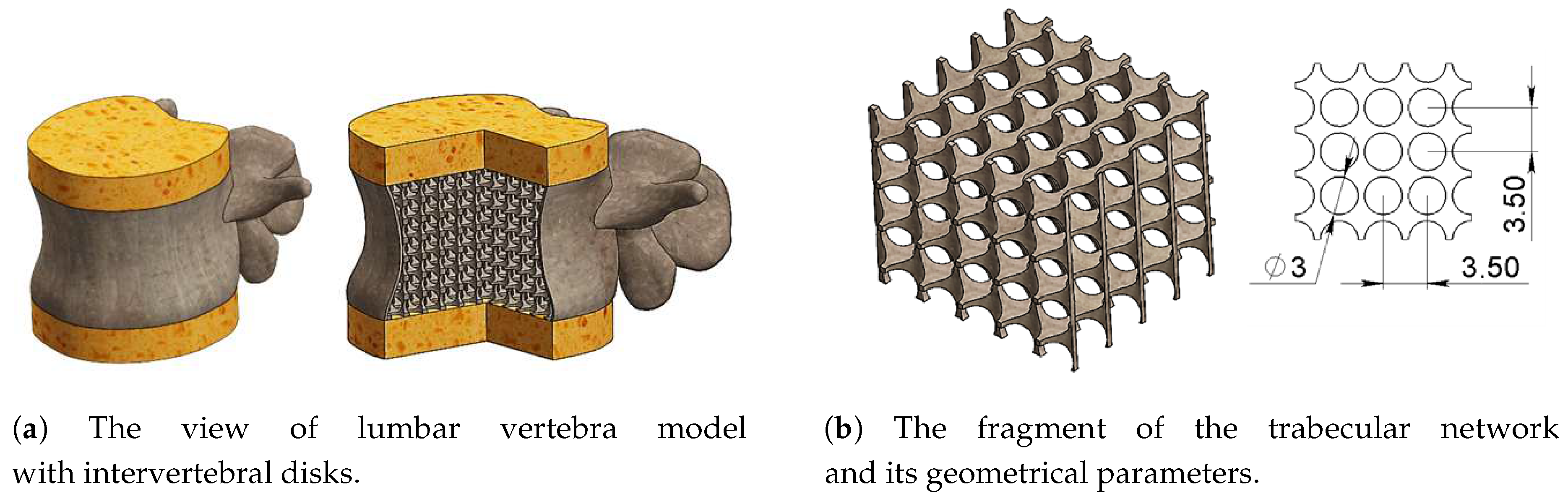
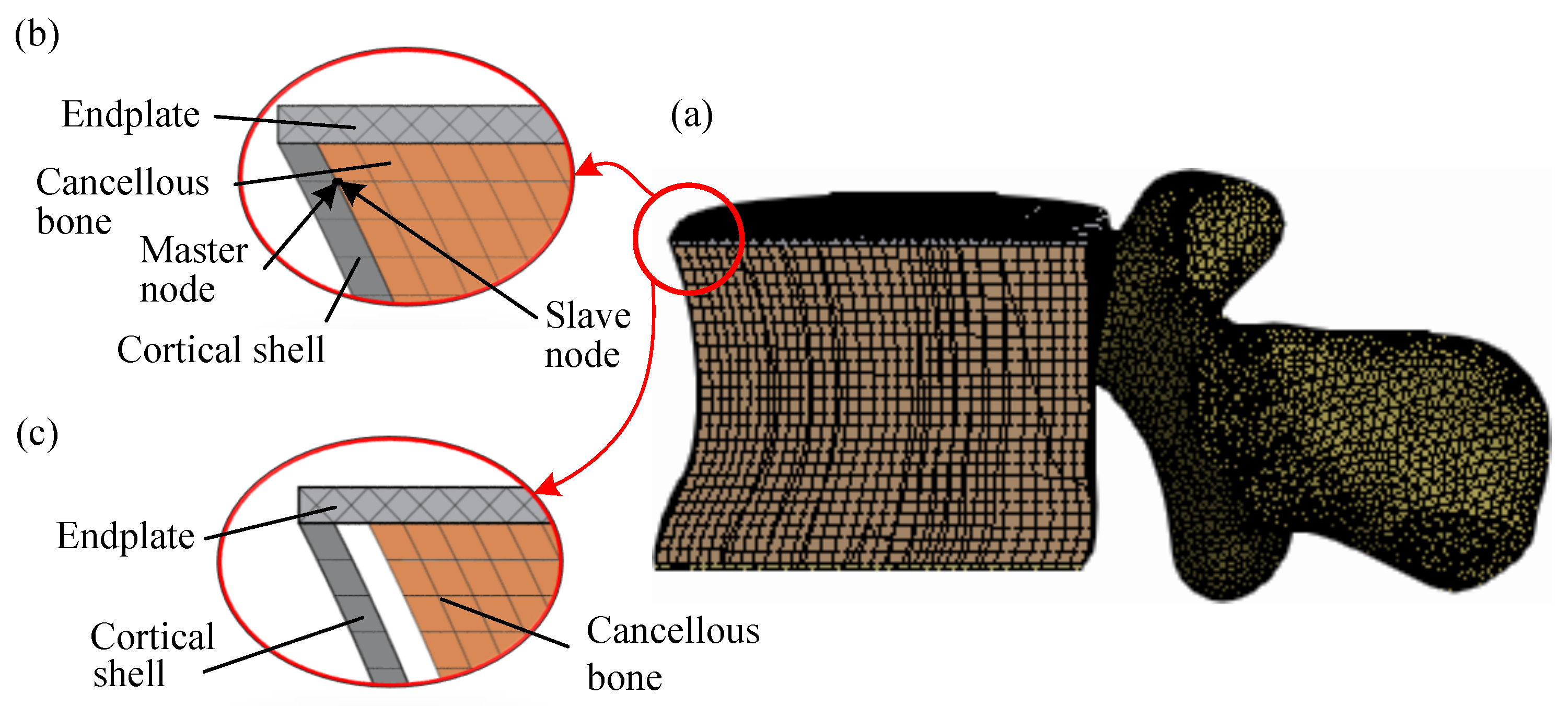
2.2. Structure and Geometrical Properties of the Model

The inhomogeneous model is made of two basic parts members: the lumbar body with posterior elements and intervertebral disks. The lumbar geometrical form is extracted by processing DICOM format data and then converted into a numerical model using Slice3D software. It is presented in Figure 1a.
The trabecular network is formed by cylindrical cuts which are extruded from vertical and horizontal planes. This method allowed the creation of the characteristic structure made of rod-like and plate-like trabeculas, and a fragment of the trabecular lattice is shown in Figure 1b.

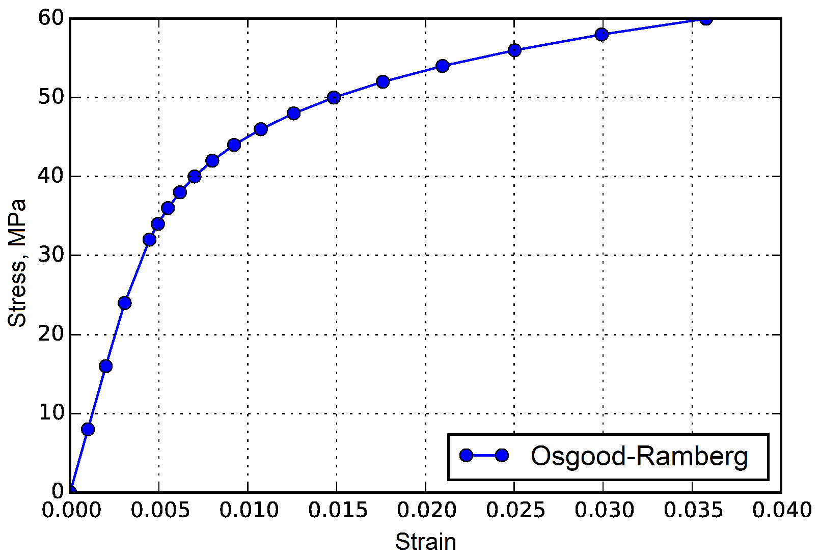
2.3. Mechanical Properties

The nonlinear stress–strain diagram of bone is presented in Figure 2. On the other hand, the intervertebral disks were considered as isotropic and perfectly elastic. The material constants of the listed components were taken from data reported by Reference [10] and presented in table Table 1.

2.4. The Parameters of Osteoporosis Impact

The effect of osteoporotic degradation is implemented by thickening the cortical bone and by varying the TBS, which depending on BV/TV. This research proposes the investigation of three parametric models with various cortical thicknesses of 0.2, 0.4, and 0.5 mm first offered in References [12,14]. Also, the relation of the BV/TV as well as the TBS value is typical for a high level of osteoporosis. The data taken from References [18,19] is presented in Table 2.
To make a profound investigation, the parameters in Table 2 were combined in different cases of calculations that were performed for both static and dynamic analyses (Table 3).

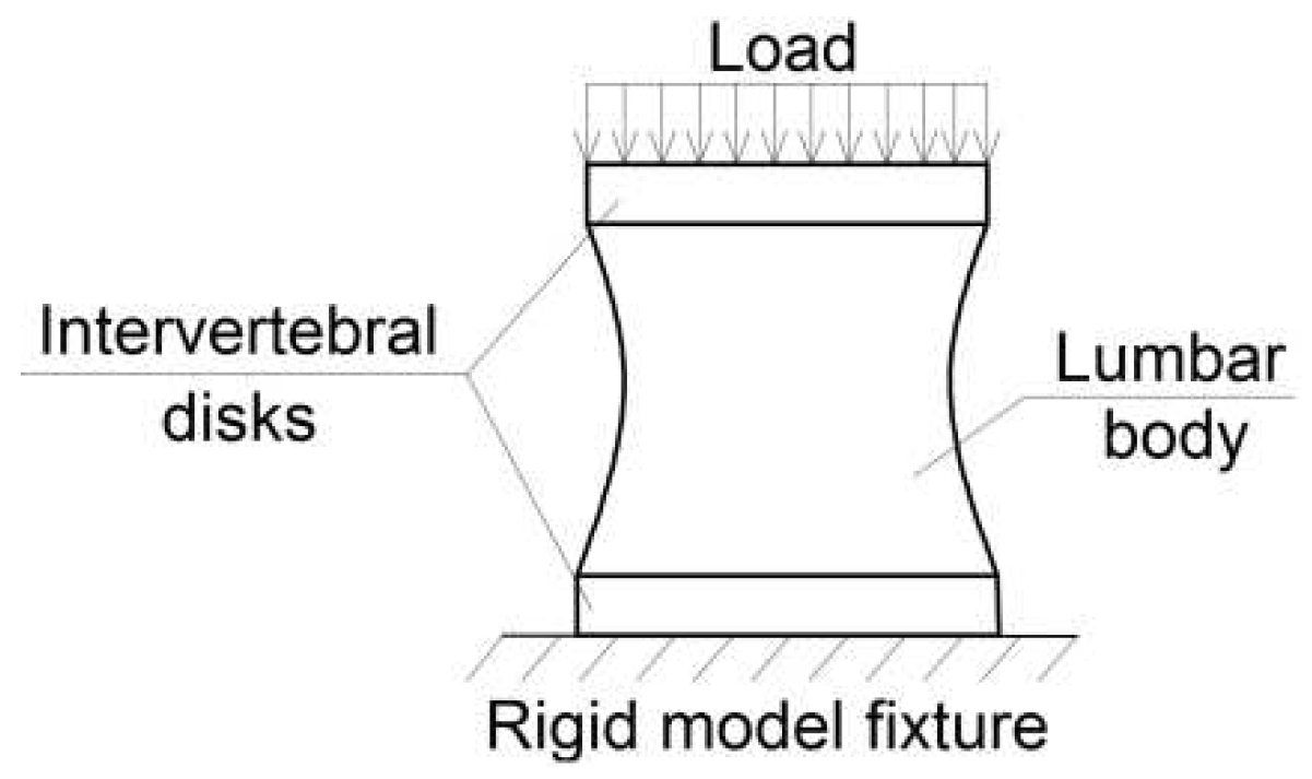
2.5. Boundary Conditions and Mesh

The model was tested by the external loads in the range of 0.15–0.75 MPa which arise in the results of daily motions [14]. The conditions of loading are reflected in Figure 3. Also, in the case of the nonlinear problem, the load direction is bonded with the displacement values and, during the test, follows the deformed shape of the model.
The time curve of the load is presented in Figure 4 and simulates the bearing of dynamic load. The time curve character comes from experimental data reported by Reference [28].
The model is meshed with tetrahedral finite elements and characterized by 306,435, 277,896, and 256,438 mesh elements for BV/TV ratios of 0.35, 0.20, and 0.1 or TBS values of 1.45, 1.33, and 1.2, respectively.
The contact between vertebra and intervertebral disks is treated as no penetration-bonded contact.

2.6. Risk Evaluation

The following three random variables were used to evaluate risk: external load P, the cortical shell thickness of lumbar vertebra Δ , and bone volume to total volume ratio β B V T V which was obtained from TBS interdependence. In contrast, TBS was obtained from the 2-D vertebra CT scan. These variables were used for solving the FEM for the proposed mechanical model strength of the lumbar vertebra. Finally, the obtained set of points values for different combinations of independent variables were used for least square fitting by cubic polynomial as follows
σ s ( β , δ , p ) = i , j , k = 0 i + j + k 3 a i j k β i δ j p k
where p is the external load, δ is the cortical shell thickness, and β is the BV/TV ratio.
Furthermore, the approximation was obtained by using logarithmic values of FEM stresses log ( σ v o n M i s e s ) by searching minima of the following expression:
min | i , j , k log ( σ v o n M i s e s ( i , j , k ) ) σ s ( β i , δ j , p k ) |
where indexes i , j , k denote values of discrete independent variables used in FEM computations.
Fracture risk F R of lumbar vertebra can be expressed in term of reliability:
R = P ( Z 0 ) = 1 F R ( Z 0 ) ,
where Z = X σ Y σ Y , X σ is max stress, and Y σ Y is yield strength. The general expression for the fracture risk of a stress–strength system has the following cumulative density function (CDF) [29]:
F R = 1 P ( Z 0 ) = 1 0 0 f X σ ( σ + z ) f Y σ Y ( σ ) d σ d z
where f X σ and f Y σ Y are probability density functions (PDFs) of the random values X σ and Y σ Y of the maximum stress caused by the external load p and the strength, respectively.

3. Numerical Results and Discussion

Important parameters that impact the state of lumbar body, such as the thickness of the cortical shell and the BV/TV relation, were combined between themselves and investigated due to various values of external load. Also, the numerical results of both static and dynamic analysis and the discussion of the results are presented in the following section.

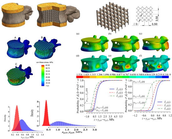
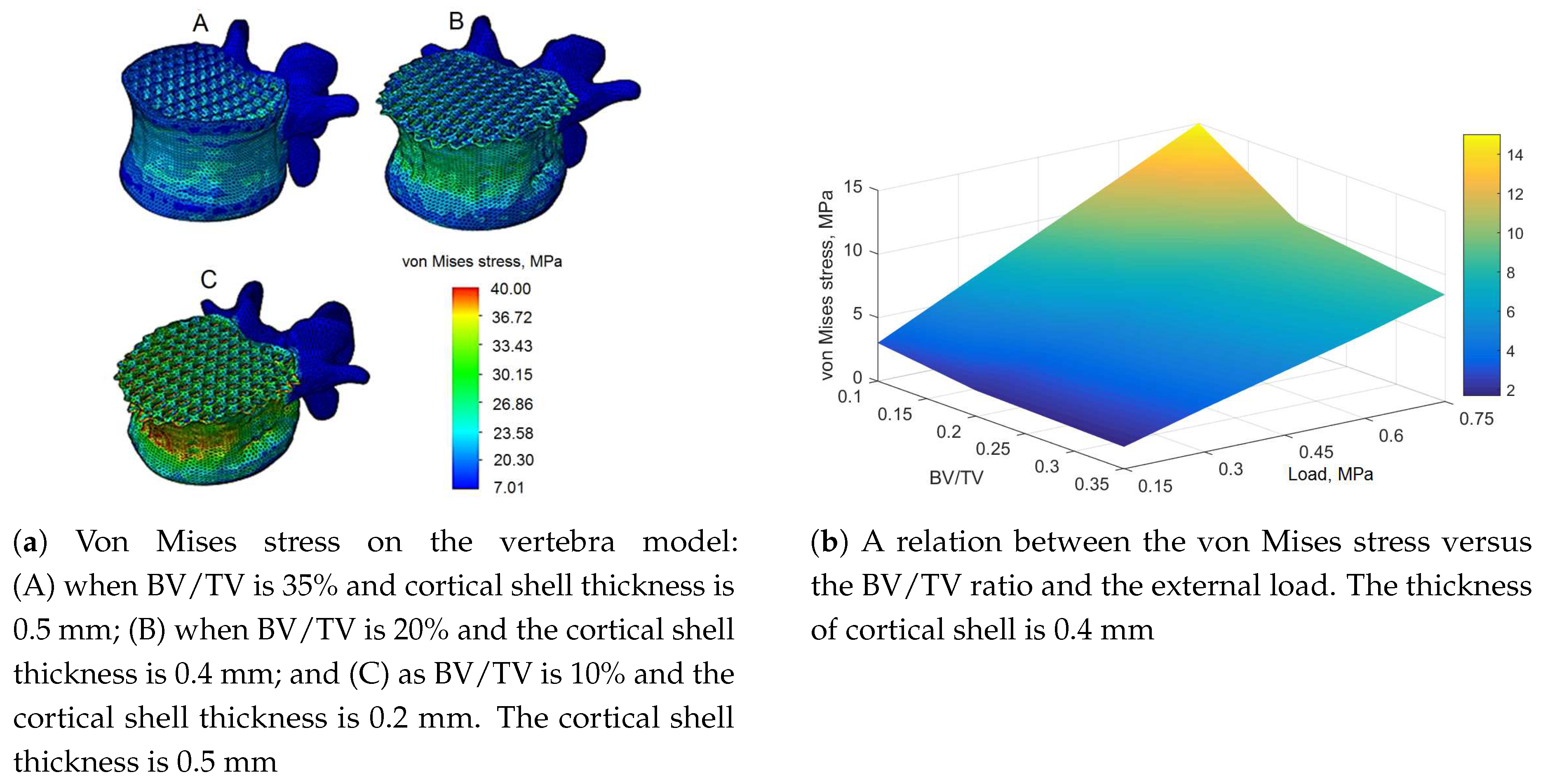
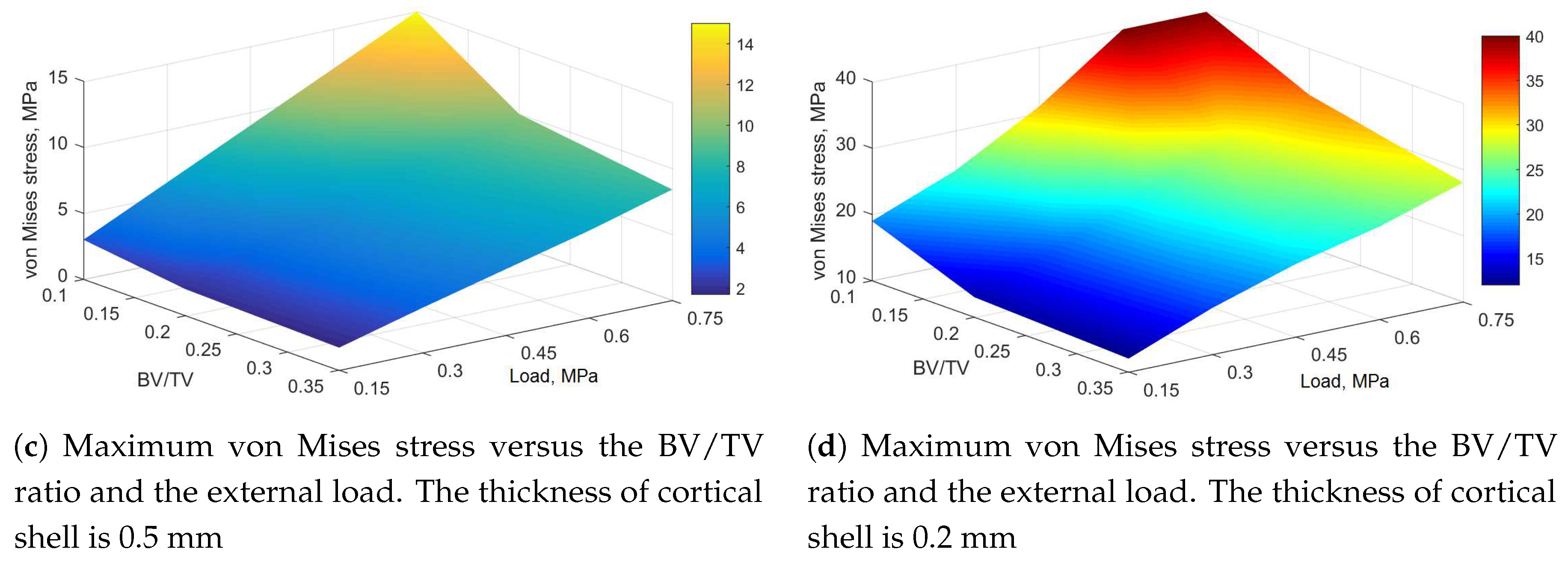
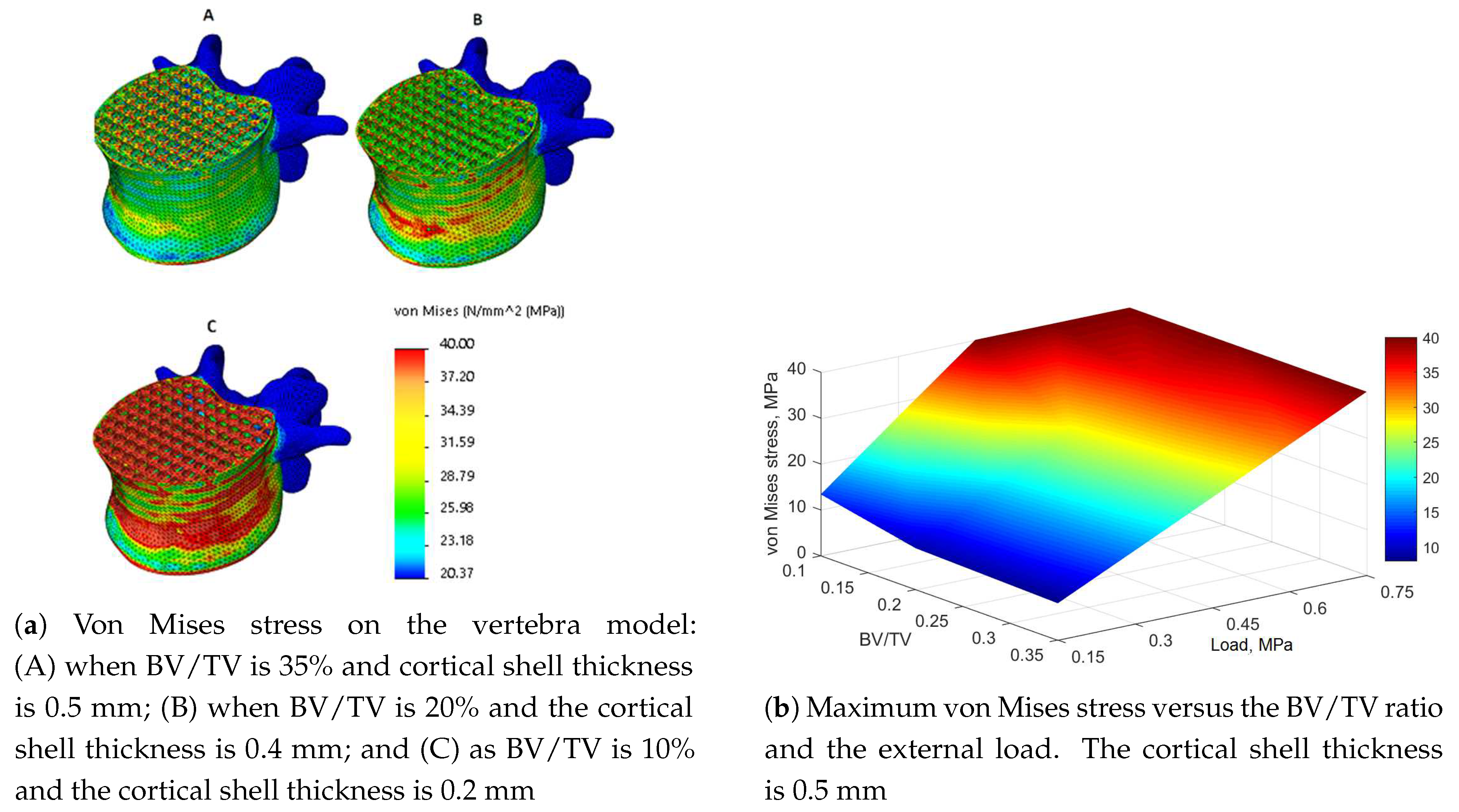
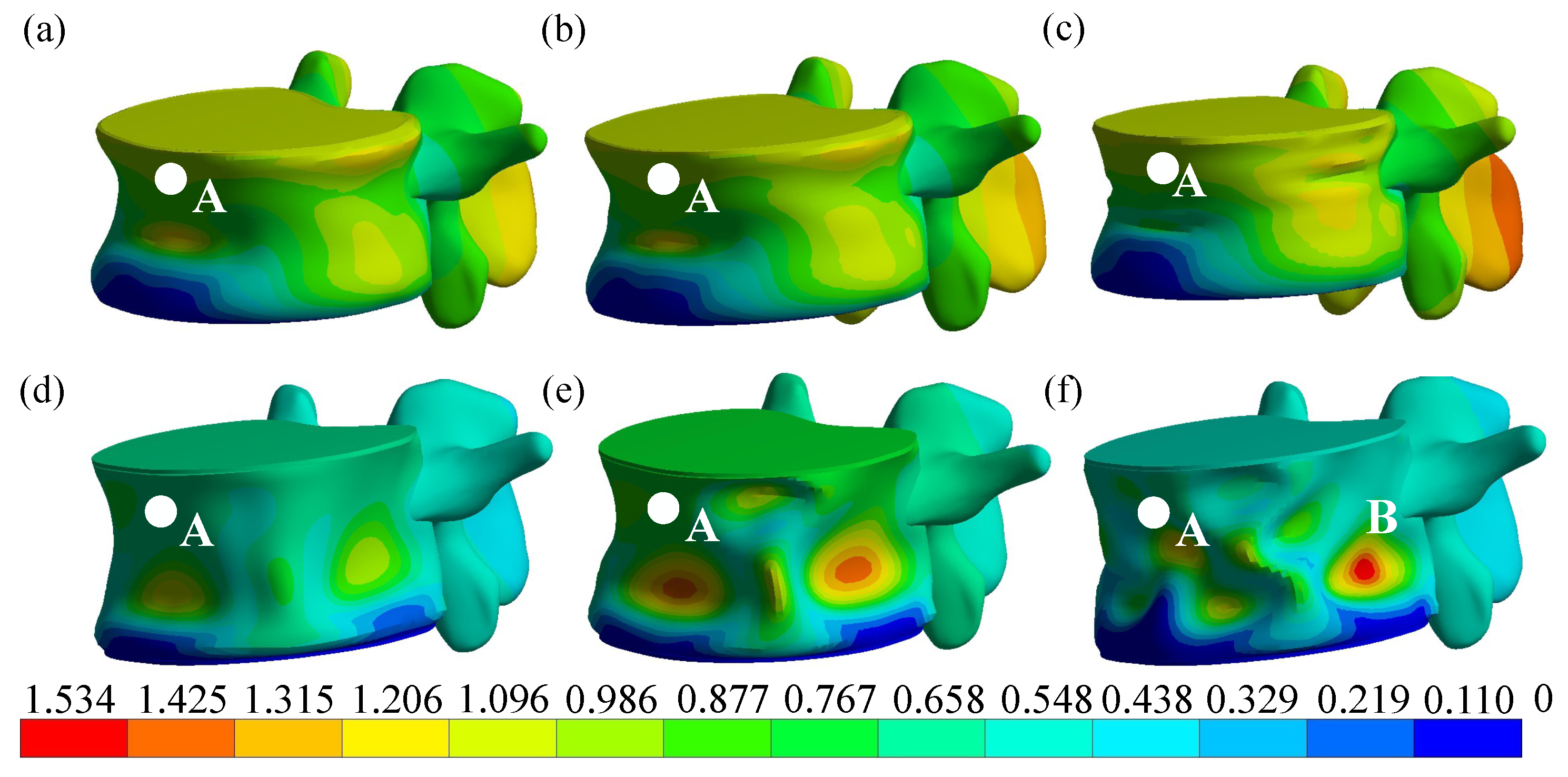
3.1. Static Analysis

Contours of the deformed shape of the model were generated, and stress distribution on the model is shown in Figure 5. The figure shows that the highest von Mises stresses occurred in the middle of the cortical shell on the front side of the model and that the deformations are scaled by a factor of 20 for visualization purposes. Figure 5b shows a relation between the von Mises stress versus the BV/TV ratio and the external load. The results show that maximal calculated stress reaches 38% of yield stress due to a 0.75 MPa load on the model with the lowest BV/TV ratio (0.1). Figure 5c,d shows the von Mises stress for models with thicknesses of cortical shell of 0.4 and 0.2 mm, respectively. In the case of a cortical shell with a thickness of 0.4 mm, maximal stress is about 17 MPa due to the minimal BV/TV ratio and the maximum external load (0.75 MPa), reaching 43% of the yield stress.
Figure 5d shows that the strength load is 0.60 MPa (the yield stress is exceeded), while the BV/TV ratio is 0.1. The obtained results agree well with the research of Kim et al., [14], with a difference about 5–10% for the model with a low apparent density and a cortical shell thickness of 0.2 mm, while McDonald [12] reports this value up to 0.99 MPa.

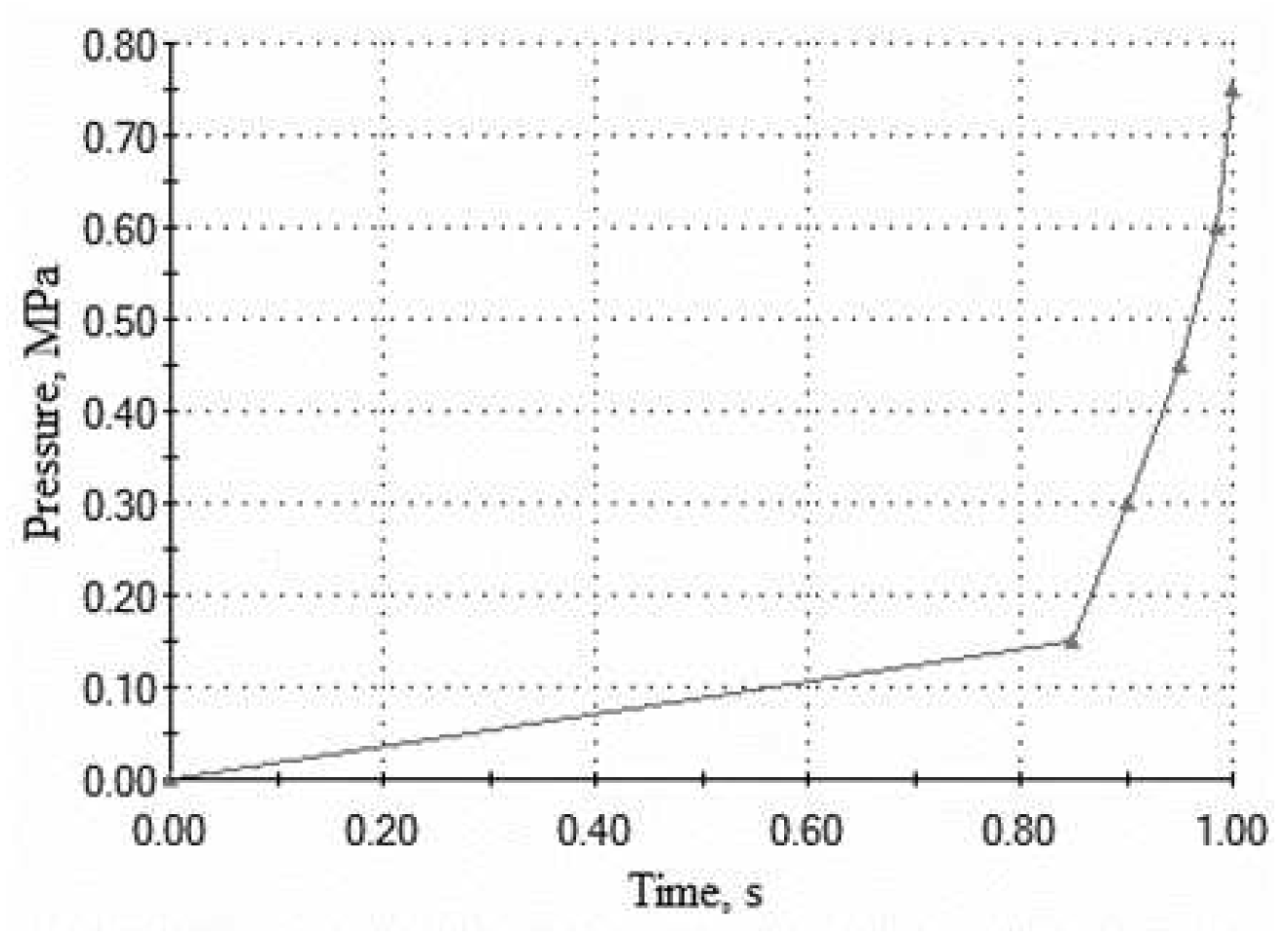
3.2. Dynamic Analysis

The stress distribution in the lumbar vertebra during dynamical analysis was computed, and the analysis shows that the stress concentrators have greater differences than seen in the static analysis. The highest value of stress appeared in the middle of the cortical shell and agrees well with clinical observations [1,2,3,4,30]. Also, the distribution of the von Mises stress on the cortical shell of the model is shown in Figure 6a. Figure 6b–d presents a relation of the von Mises stress on the model versus the BV/TV ratio and the external load. Figure 6d shows that yield stress is exceeded due to the 0.45 MPa load while the BV/TV ratio is less than 0.1. The relations between the von Mises stress on the cortical shell of the model with thicknesses of 0.4 and 0.2 mm versus the BV/TV ratios and the external load are presented in Figure 6c,d, respectively.
As shown in Figure 6c, the excess yield stress is expected due to the 0.45 MPa load, while the BV/TV ratio is minimal. In the case of a high BV/TV ratio, the excess yield stress was identified due to the load of 0.6 MPa in terms of the average thickness of the cortical shell (0.4 mm). Figure 6d shows that yield stress is exceeded almost in every sample of bone tissue if the load is higher than 0.3 MPa. In addition, if the load grows increases 0.3 MPa, the yield stress is reached even in the case of a sufficient BV/TV ratio (0.35). This effect can be explained by the low thickness of the cortical shell (0.2 mm).

3.3. Estimation of the Fracture Risk

The risk of fracture of the lumbar vertebra can be estimated by the Monte Carlo method as a probability P r f = P r ( Z 0 ) , where Z = Y p , R X p , E and X p , E and Y p , R are external pressure p imposed on the vertebra and the load-bearing capacity of the vertebra random variables respectively. It is assumed that the load-bearing capacity of the vertebra p R equals the minimum pressure p at which the maximum von Mises stresses equal the yield stress σ Y , that is, for the given δ and β , the load-bearing capacity r.v. p R = m i n { p : g F E M ( δ , β , p ) σ Y } . It is assumed that X p , E and Y p , R are independent random variables. To evaluate the fracture risk P r f , the random numbers of the acting pressure random variable X p , E can be generated directly, while the generation of the random numbers of the load-bearing capacity Y p , R is more complicated since it is known that the cortical shell thickness and BV/TV are dependent random variables. In addition, the load-bearing capacity function of the lumbar vertebra p R = h ( δ , β , σ Y , ) dependent of all variables must be known. Then, the r.v. of the load-bearing capacity Y p , R can be obtained as a transformation Y p , R = h ( X δ , X β , X σ , Y , ) , where X δ , X β , X σ , Y , … are random variables affecting the load-bearing capacity of the lumbar vertebra: for example, the cortical shell thickness, BV/TV ratio, the yield stress, geometry, and so on. It is evident that it is not possible to generate the sample of the realizations of the load-bearing capacity r.v. Y p , R directly by calculating each random number by FEM. Therefore, in the present article, another approach is adopted: to approximate the maximum von Mises stresses of the vertebra by the polynomial g ^ and then, by solving this polynomial as an equation σ Y = g ^ ( δ , β , p ) , to obtain the pressure p that corresponds to the given variables δ , β , and the maximum von Mises stress σ Y .

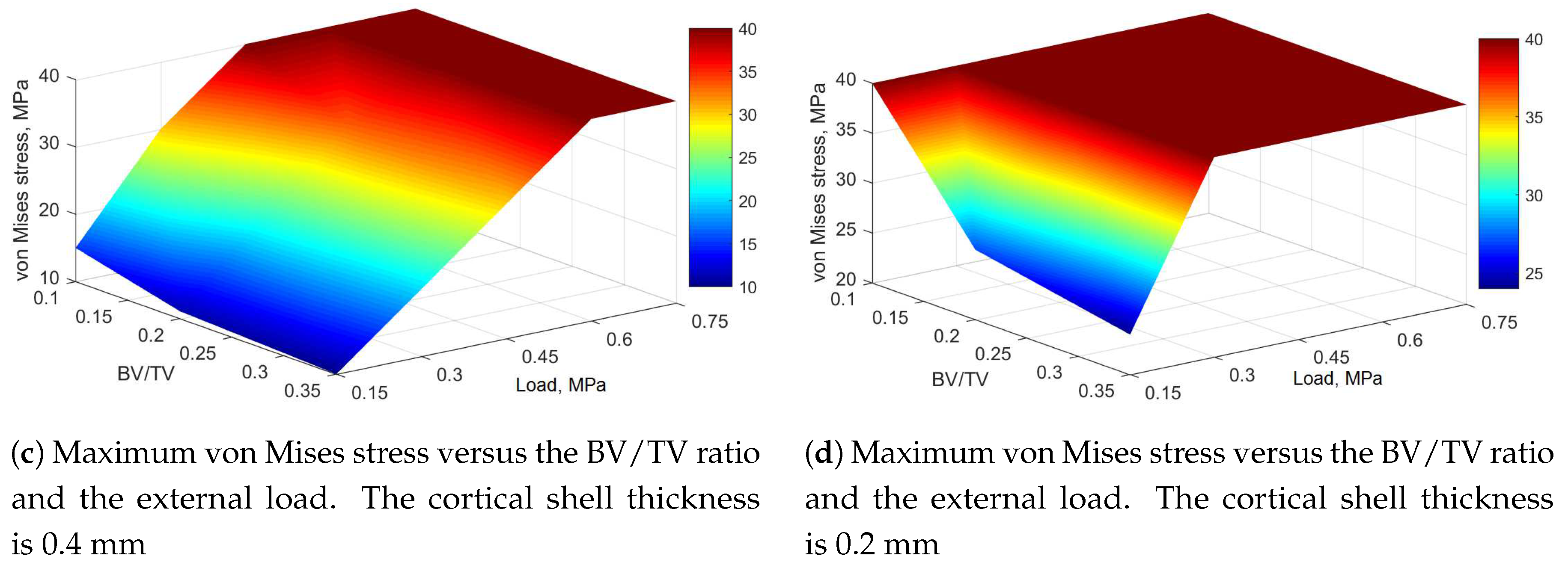
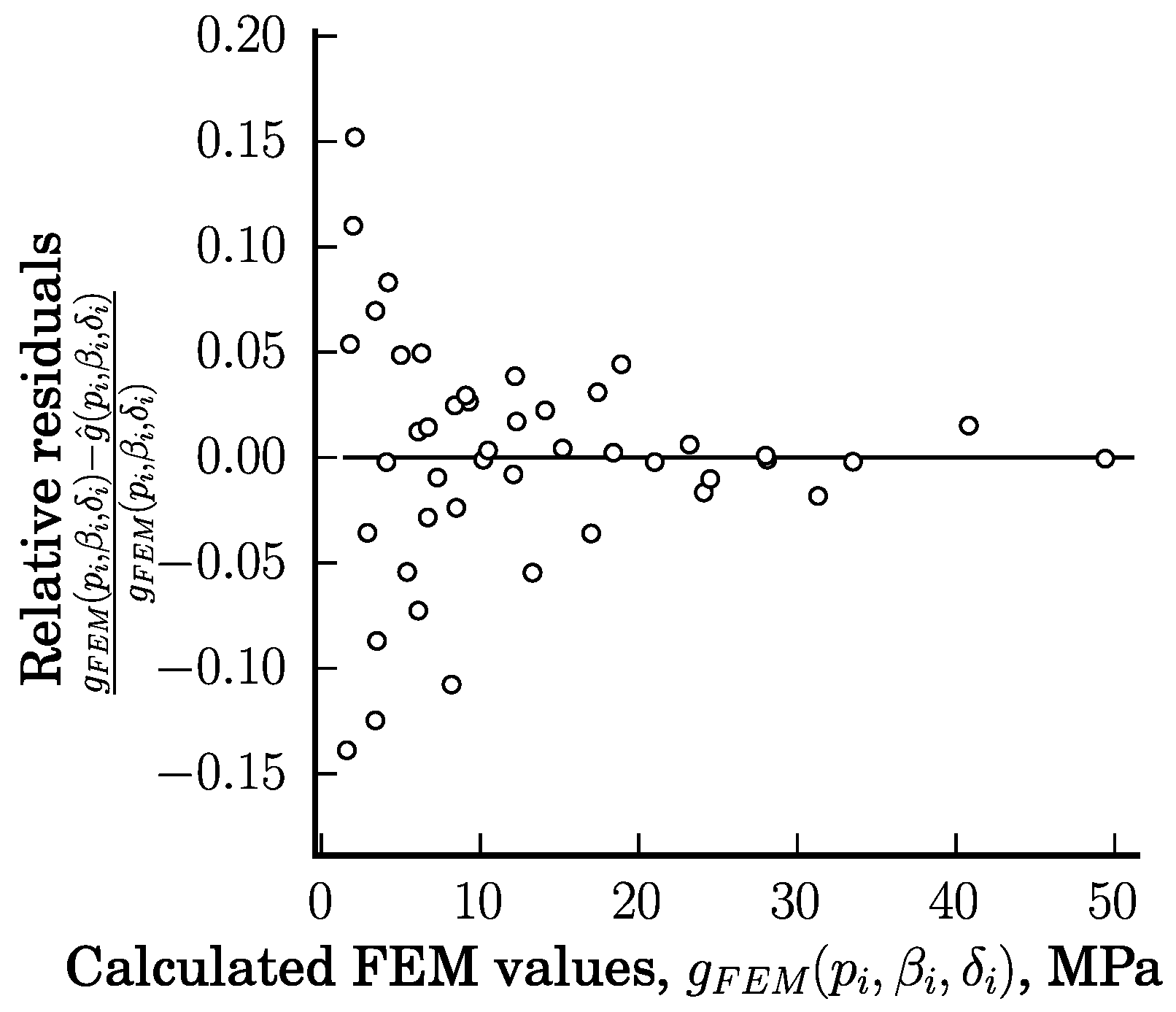
3.3.1. Approximation of the Maximum von Mises Stress

The approximation of the calculated maximum von Mises stresses of the lumbar vertebra was conducted by using the program “R studio” [31] and the package “nlme” [32] over the set D × B × P , where D , B , and P are sets of values of the cortical shell thickness δ , BV/TV ratio β , and the external load p, respectively: δ D = { 0.5 , 0.4 , 0.2 } mm, β B = { 0.1 , 0.2 , 0.35 } , and p P = { 0.15 , 0.30 , 0.45 , 0.60 , 0.75 } MPa. The set of 45 points of the maximum von Mises stresses D × B × P of the static analysis obtained by the finite element method that were used to obtain the approximating polynomial is given in Table 4.
The approximating polynomial of the maximum von Mises stresses of the static analysis is as follows:
σ g ^ ( p , β , δ ) = a 0 + a 1 p + a 2 β + a 3 δ + a 11 p 2 + a 33 δ 2 + a 12 p β + a 13 p δ + a 123 p β δ + a 112 p 2 β + a 113 p 2 δ + a 221 β 2 p + a 223 β 2 δ + a 331 δ 2 p + a 332 δ 2 β + a 12233 p β 2 δ 2 + a 11233 p 2 β δ 2 , δ [ 0.2 , 0.5 ] mm , β [ 0.1 , 0.35 ] , p [ 0.15 , 0.75 ] Mpa
where the coefficients are as follows: a 0 = 40.095 , a 1 = 109.545 , a 2 = 33.064 , a 3 = 153.799 , a 11 = 56.976 , a 33 = 152.808 , a 12 = 410.969 , a 13 = 348.377 , a 123 = 704.586 , a 112 = 153.953 , a 113 = 117.969 , a 221 = 737.456 , a 223 = 97.428 , a 331 = 361.940 , a 332 = 56.473 , a 12233 = 2913.652 , and a 11233 = 702.954 .
It should be noted that only the coefficients a i for which the statistical hypothesis H 0 : a i = 0 is rejected and the alternative H 1 : a i 0 is accepted are present in the given approximating polynomial Equation (9). The hypotheses were tested using the Student t-test. The maximum and minimum residuals are as follows: m a x { g F E M ( p i , β i , δ i ) g ^ ( p i , β i , δ i ) } = 0.883 MPa and m i n { g F E M ( p i , β i , δ i ) g ^ ( p i , β i , δ i ) } = 0.838 MPa, where ( p i , β i , δ i ) D × B × P and g F E M ( p i , β i , δ i ) stand for the stress values calculated by the FEM. The relative residuals ( g ^ ( p i , β i , δ i ) g F E M ( p i , β i , δ i ) ) / g F E M ( p i , β i , δ i ) versus the stresses calculated by FEM are depicted in Figure 7.
The obtained polynomial g ^ , given in Equation (9), can be treated as a quadratic equation σ Y = g ^ ( p , β , δ ) with respect to the pressure p when the other two variables δ and β are treated as known quantities or, in other words, as the parameters. Then, the solution of the obtained polynomial g ^ , given in Equation (9), gives two roots: One of them is the load-bearing capacity p R corresponding to the given δ , β , and the yield stress σ Y :
p R h ^ ( β , δ ) = b 1 ( β , δ ) + b 1 ( β , δ ) 2 4 b 2 ( β , δ ) ( b 0 ( β , δ ) σ Y ) 2 b 2 β , δ
where b 0 ( β , δ ) = a 332 β δ 2 + a 33 δ 2 + a 223 β 2 x 3 + a 3 δ + a 2 β + a 0 , b 1 ( β , δ ) = a 12233 β 2 δ 2 + a 331 δ 2 + a 123 β δ + a 13 δ + a 221 β 2 + a 12 β + a 1 and b 2 ( β , δ ) = a 11233 β δ 2 + a 113 δ + a 112 β + a 11 .
Then, the load-bearing capacity r.v. Y p , R can be modelled as the transformation Y p , R = h ^ ( X β , X δ ) of r.vs. X β and X δ by assuming that the yield stress σ Y is the deterministic predefined quantity.

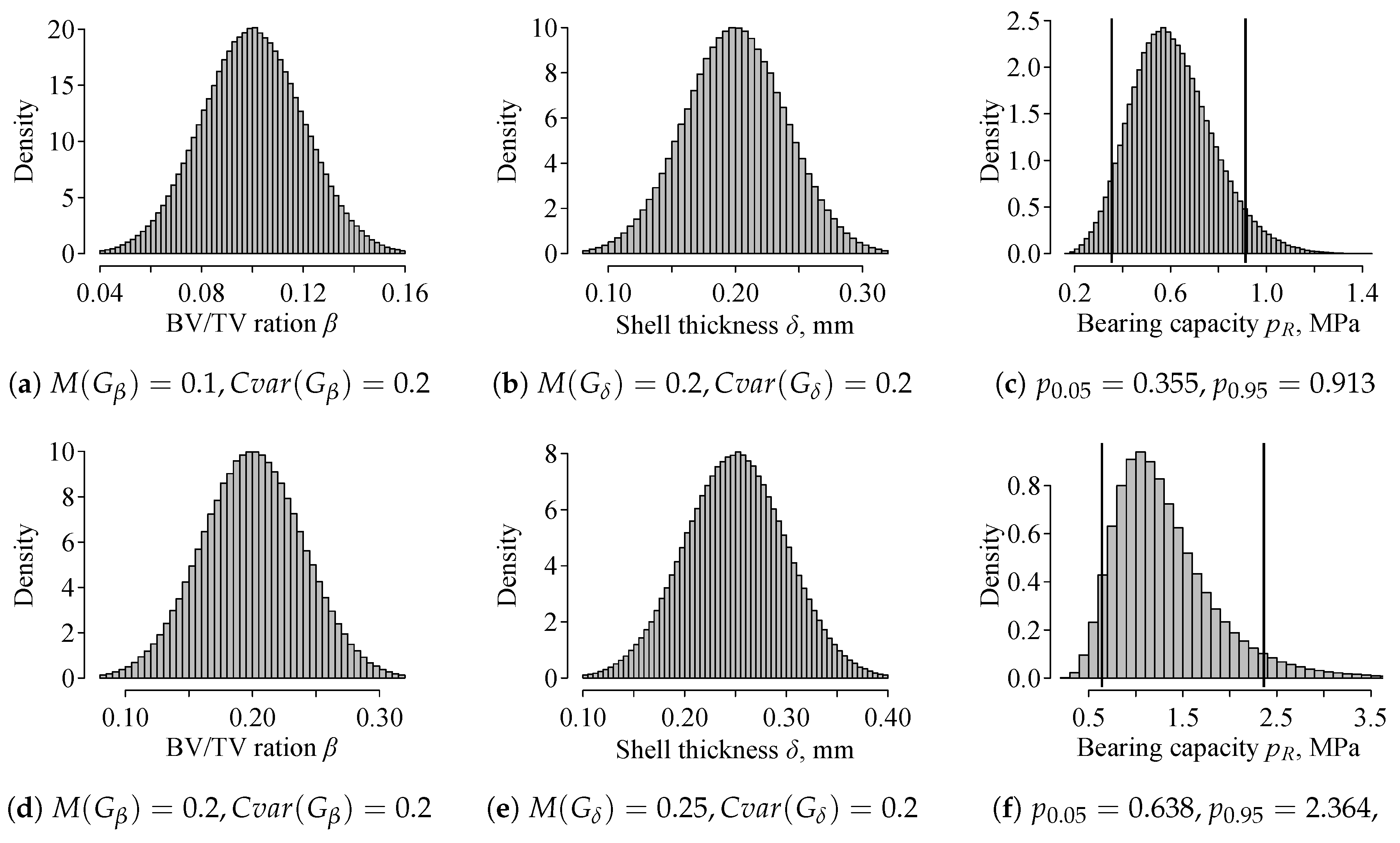
3.3.2. Stochastic Models and for the Risk Modelling

It is well-known that osteoporosis of the trabecular bone also entails decreasing of the thickness of the cortical shell of the lumbar vertebra δ . Therefore, BV/TV and the cortical shell thickness are dependent random variables. In addition, decreasing BV/TV also entails decrease of the cortical shell thickness δ [33,34]. Therefore, the correlation coefficient of these r.vs. is positive. For example in Reference [33], it is obtained that the statistically significant coefficient of correlation between the cortical shell thickness and BV/TV is 0.5 , when the significance level is 0.05. According to Reference [34], the coefficient of correlation between BV/TV and the cortical shell thickness is 0.29 ; however, it is statistically insignificant. To generate the load-bearing capacity X p , R random numbers, it is assumed that the BV/TV ratio and the cortical shell thickness form a bivariate correlated truncated Gaussian random variable ( X β , X δ ) T [ M ( G β ) 3 D ( G β ) , M ( G β ) + 3 D ( G β ) ] × [ M ( G δ ) 3 D ( G β ) , M ( G β ) + 3 D ( G β ) ] ; where × is the Cartesian product of two sets; M ( G β ) , D ( G β ) , M ( G δ ) , and D ( G δ ) are the means and variances of the correlated untruncated normal random variables G β and G δ , respectively, that also form a bivariate Gaussian random variable ( G β , G δ ) T N ( μ , Σ ) of which the mean vector is μ = ( M ( G β ) , M ( G δ ) ) T and the covariance matrix is
Σ = D ( G β ) C o r ( G β , G δ ) D ( G β ) D ( G δ ) C o r ( G δ , G β ) D ( G δ ) D ( G β ) D ( G δ )
where C o r ( G β , G δ ) and C o r ( G δ , G β ) are the correlation coefficients between r.vs. G β and G δ , C o r ( G β , G δ ) = C o r ( G δ , G β ) .
R.v. Y p , R can be estimated by the empirical cumulative distribution function (ECDF) and by the empirical quantile function (EQF). Usually, ECDF is defined as follows: P r ( Y p , R y ) F ^ Y , p , R ( y ) = 1 n i = 1 n I ( y i y ) , where I is the indicator function, n is the sample size, y i is the realization i of r.v. Y p , R ; while EQF of r.v. Y p , R is usually defined as Q ( p ) = i n f { y : F Y , p , R ( y ) p } , where p is the required probability.
For the evaluation of the fracture risk as the probability P r f = P r ( Y p , R X p , E 0 ) , the external pressure independent r.v. X p , E can distributed according to various laws. In the present article, it is assumed that the external load r.v. X p , E is also truncated normal r.v. attaining values from the interval X p , E [ M ( G p , E ) 3 D ( G p , E ) , M ( G p , E ) + 3 D ( G p , E ) ] , where M ( G p , E ) and D ( G p , E ) are the mean and the variances of the untruncated external pressure normal r.v. G p , E .
The fracture risk of the lumbar vertebra can be expressed as P r f = P r ( Y p , R X p , E 0 ) = P r ( Z 0 ) F ^ Z ( 0 ) , where F ^ Z is the ECDF of r.v. Z = Y p , R X p , E : F ^ Z ( z ) = 1 n i = 1 n I ( y p , R , i x p , E , i z ) , where n is the sample size and y p , R , i and x p , E , i are realization i of r.vs. Y p , R and X p , E , respectively. It should be noted that the fracture risk can be also evaluated according to the following known integral [29]:
P r f = P ( Z 0 ) = 0 + f Y , p , R ( p + z ) f X , p , E ( p ) d p d z
where f Y , p , R and f X , p , E are probability density functions (PDFs) of the load-bearing capacity r.v. Y p , R and the external presure r.v. X p , E , respectively.
For the following analysis of the reliability of the vertebra, the concrete parameters of the r.v. G β , G δ , and G p , E must be adopted. In the case of the Gaussian r.vs., only the means, variances, and covariances are required. The coefficient of variation C v a r ( G β ) of BV/TV can vary in a wide range, for example, from about 18 % [18,33] up to 37 % [34] or even up to 42 % for the normal bones [26]. There is less literature on the coefficient of the variation of the cortical shell thickness δ . We found that the coefficient of variation is also big, for example, 24.5 % [33] or even 62.4 % , according to Reference [34]. For the patient-specific cases, the variability of these parameters should be less. However, since the BV/TV ratio is determined indirectly, the variability of r.v. X β cannot be very low.
As it was already mentioned, the r.vs. X β and X δ are dependent [33,34]. In the case of the Gaussian bivariate r.v. ( G β , G δ ) , the correlation coefficient C o r ( G δ , G β ) is used in the covariance matrix given in Equation (11) and it is determined that C o r ( G δ , G β ) may equal 0.5 [33] or 0.29 [34]. The external load X p , E acting on the vertebra is a random variable depending mainly on the mechanical loads. For example, according to Reference [28], the ground reaction of a human may vary from 750 N in the rest state and increases up to 2000 N in the squat jump. The ground reaction of the rest state shows that the mass of the investigated human body in Reference [28] is about 75 kg. Then, in the squat jump, the weight of the body increases 2000 / 750 = 2.66 ( 7 ) times. It should be mentioned that not all the weight of a body is imposed on the lumbar vertebra. On the basis of the data given in Reference [35], it is possible to conclude that a lumbar vertebra sustains about 60 % of the total load. By taking into account the area of the loaded surface of the vertebra under investigation, A = 1210 mm 2 , we can conclude that, for the person of article [28], the external load varies within an interval [ p m i n , p m a x ] = [ 0.372 , 0.992 ] MPa.

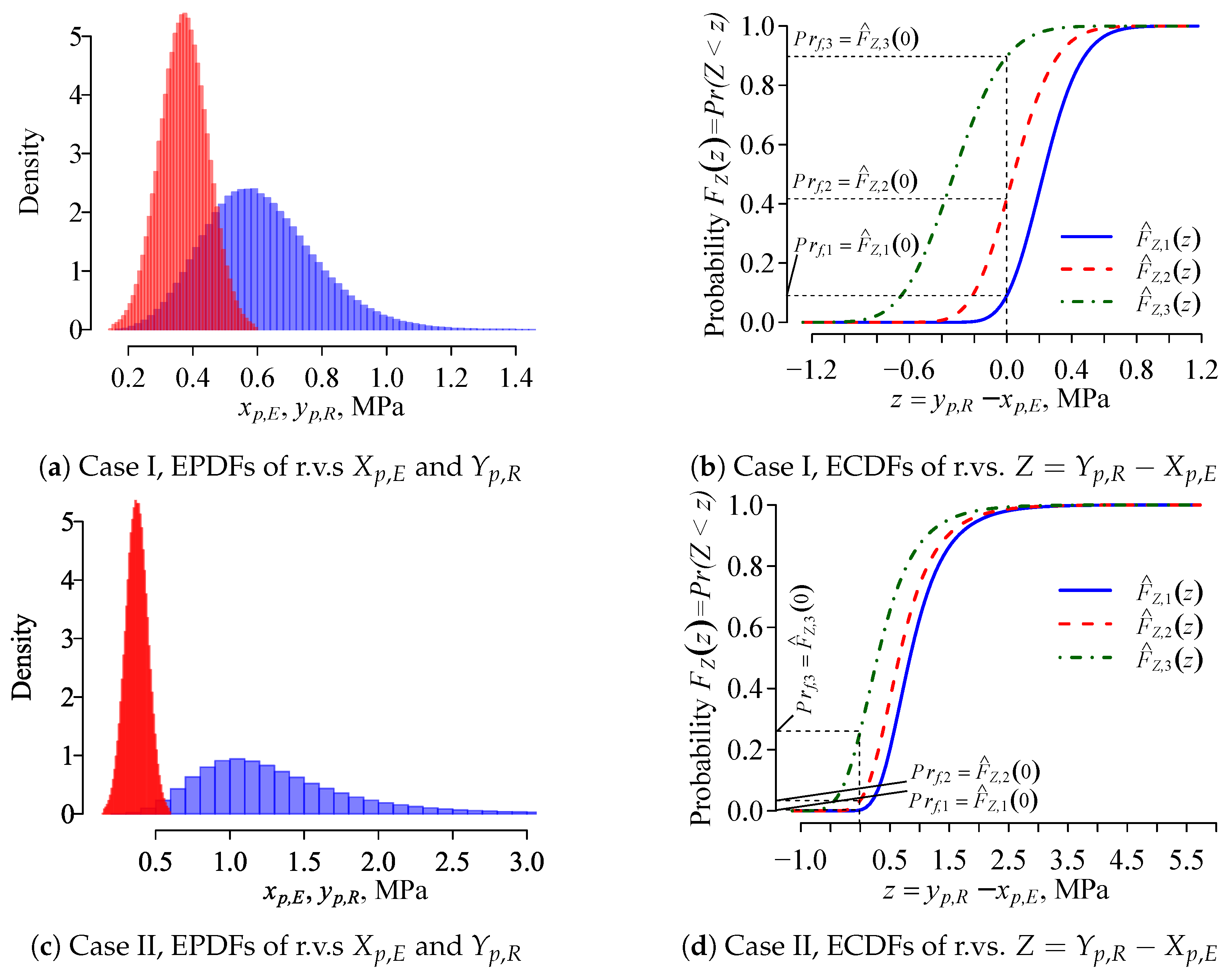
3.3.3. Fracture Risk Modelling Data, Results, and Discussion

On the basis of the above given review, for the probabilistic estimations of the load-bearing capacity of the lumbar vertebra P r ( Y p , R y p ) = F ^ Y , p , R ( y p ) and the failure risk P r f = P r ( Z 0 ) = F Z ( 0 ) , the following two cases were considered. For the first case (Case I), the following values are adopted: the mean of BV/TV M ( G β ) = 0.1 and the mean of the cortical shell thickness M ( G δ ) = 0.2 mm; the coefficients of variation C v a r ( G β ) = D ( G β ) / M ( G β ) = 0.2 and C v a r ( G δ ) = 0.2 ; the correlation coefficient C o r ( G β , G δ ) = 0.35 ; the mean of the external load G p , E attains three values M ( G p , E ) { p m i n , 1.5 p m i n , 2.5 p m i n } , where p m i n = 0.372 Mpa; and the coefficient of variation for all external pressures is constant: C v a r ( G p , E ) = 0.20 . For the second case (Case II), the following values are adopted: means M ( G β ) = 0.25 and M ( G δ ) = 0.2 mm; the coefficients of variation C v a r ( G β ) = 0.2 and C v a r ( G δ ) = 0.2 ; the correlation coefficient C o r ( G β , G δ ) = 0.35 ; mean of the external load G p , E attains three values M ( G p , E ) { p m i n , 1.5 p m i n , 2.5 p m i n } , where p m i n = 0.372 Mpa; and the coefficient of variation for all external pressures is constant: C v a r ( G p , E ) = 0.2 . Thus, for both Cases I and II, the external load G p , E attains the same three different means and the coefficient of variation is constant, and for both cases, the coefficient of the correlation between the cortical shell thickness and BV/TV is the same, 0.35. It should be noted that for Cases I and II the mean of the external pressure M ( G p , E ) = 0.372 MPa approximately corresponds to the external load of the lumbar vertebra of a person of mass 75 kg in rest, while M ( G p , E ) = 2.5 p m i n = 0.93 MPa is close to the maximum load during the squat jump of the person. Totally, 10 6 random values of the r.vs. G β and G δ were generated. However, due to the truncation the samples of the realizations of the r.vs. X β , X δ , X p , E , and Y p , R were smaller than 10 6 but bigger than 9 × 10 5 . All analyses were performed by the program “R studio” [31]. The bivariate Gaussian random numbers were generated using the package “MASS” [36].
The realizations of the histograms of the r.vs. X β , X δ and Y p , R are shown in Figure 8. The realizations of the histograms of the truncated BV/TV ratio r.v. X β are depicted in Figure 8a,d and the realizations of the truncated cortical shell thickness r.v. X δ are depicted in Figure 8b,e while realizations of the histograms of the load-bearing capacity r.v. Y p , R as well as the 0.05 and 0.95 empirical quantiles of r.v. Y p , R are depicted in Figure 8c,f. It should be noticed that the histograms depicted in Figure 8a,b,d,e show entire ranges of the random numbers of the r.vs. X β and X δ , while Figure 8c,d show truncated ones from the right of the intervals of r.vs. Y p , R .
As we can see from Figure 8c,f, the probability density function of the load-bearing capacity r.v. Y p , R can have a positive skew. However, there are such cases of M ( X β ) , M ( X δ ) , D ( X β ) , and D ( X δ ) in which the histograms of r.v. Y p , R have a negative skew. It was also observed that at the small values of variances D ( X β ) and D ( X δ ) , the histograms of the r.v. Y p , R are symmetrical and the histograms are very similar to the normal distribution probability density function with mean M ( Y p , R ) and variance D ( Y p , R ) . However, the given Figure 8c,f shows a counterexample, and in general, we cannot state that r.v. Y p , R is normal provided that r.vs. X β and X δ are symmetrically truncated dependent normal random variables with nonnegative correlation coefficient. As we can see from Figure 8c,f, the 0.05 quantiles of the load-bearing capacity of the vertebra r.v. Y p , R increase from p 0.050 = 0.355 MPa for Case I up to p 0.05 = 0.638 MPa for Case II. Analogously, the 0.95 quantiles increase from p 0.95 = 0.913 MPa up to p 0.95 = 2.364 MPa. The quantiles of the load-bearing capacity r.v. Y p , R can serve as extra information on the fracture risk of the lumbar vertebra. It should be noted that the correlation between r.vs. X β and X δ in general is important for r.v. Y p , E . For example, for the considered Case I, the increase of the correlation coefficient C o r ( G β , G d e l t a ) from 0.35 up to 0.5 decreases the small quantiles of the load-bearing capacity r.v. Y p , R from p 0.05 = 0.355 up to p 0.05 = 0.347 and increases the big quantiles from p 0.05 = 0.913 up to p 0.95 = 0.929 . For Case II, the increase the correlation coefficient from C v a r ( G β , G δ = 0.35 ) up to C v a r ( G β , G δ ) = 0.5 also entails a decrease of small value quantiles of r.v. Y p , R from p 0.05 = 0.638 up to p 0.05 = 0.620 , but the increase in the correlation coefficient also increases the big quantile values from p 0.95 = 2.364 up to p 0.95 = 2.423 .
The fracture risks of static vertebra loads of Case I and Case II as well histograms of r.vs. Y p , R , X p , E , and Z = Y p , R X p , E can be seen in Figure 9. It was obtained that with increasing the cortical shell thickness from δ = 0.2 (Case I) to δ = 0.25 (Case II) and the BV/TV ratio from β = 0.1 (Case I) to β = 0.2 (Case II), the failure risk P r f decreases from 0.0904 to 2.752 · 10 3 for M ( G p , E ) = p m i n = 0.372 MPa; from 0.417 to 0.0337 for M ( G p , E ) = 1.5 p m i n = 0.558 MPa; and from 0.897 to 0.260 for M ( G p , E ) = 2.5 p m i n = 0.93 MPa. The obtained results suggest that, for the considered supposed person, the squat jump inevitably would lead to the fracture of a lumbar vertebra, while a relatively small increasing BV/TV and the cortical shell thickness δ significantly decrease the fracture risk P r f .
The correlation between r.vs. X β and X δ is also important for the fracture risk P r f . For example, for the considered Case I, the increase of the correlation coefficient C o r ( G β , G δ ) from 0.35 up to 0.5 increases the fracture risk from P r f = 0.0904 up to P r f = 0.0963 and from P r f = 0.417 up to P r f = 0.418 at small values of the loading, i.e., as M ( G p , E ) { p m i n , 1.5 p m i n } = { 0.372 , 0.558 } MPa. However, at big load values, the increasing correlation coefficient decreases the fracture risk from P r f = 0.897 up to P r f = 0.892 as M ( G p , E ) = 2.5 p m i n = 0.93 MPa. For Case II, the increase in the correlation coefficient from C v a r ( G β , G δ = 0.35 ) up to C v a r ( G β , G δ ) = 0.5 increases the fracture risk from P r f = 0.002752 up to P r f = 0.00387 as M ( G p , E ) = p m i n = 0.372 MPa; from P r f = 0.0337 up to P r f = 0.0392 as M ( G p , E ) = 1.5 p m i n = 0.558 MPa; and from P r f = 0.260 up to P r f = 0.270 as M ( G p , E ) = 2.5 p m i n = 0.93 MPa.
It should be noted that the probabilistic evaluation of the fracture risk demands information on the probability distribution functions of the many variables that affect the failure of a lumbar vertebra such as BV/TV ratio, the cortical shell thickness, yield strength of bone, geometric parameters, and so on. These variables should be treated as the random variables, and in addition, as it was already mentioned, these random variable are dependent. Therefore, at least the correlation coefficients or covariances between these random variables should be known. However, we could not find any information about the probability distribution laws of the mentioned variables that affect lumbar vertebra fracture. Therefore, the Gaussian laws were applied to the modelling.
The proposed model can be used to determine the fracture risk of individual patients by applying the peculiar anatomical properties of lumbar vertebrae, such as TBS or BV/TV. So, the proposed evaluation scheme of assessing fracture risk includes the model of a vertebra with cancellous bone and the cortical shell, in-silico numerical results obtained by using FEM software, and the basic expressions of evaluating the fracture risk of a mechanical system. In case of the existence of other universally recognized methods, our proposed method can be used as a supplementary method with other known fracture risk evaluation methods.

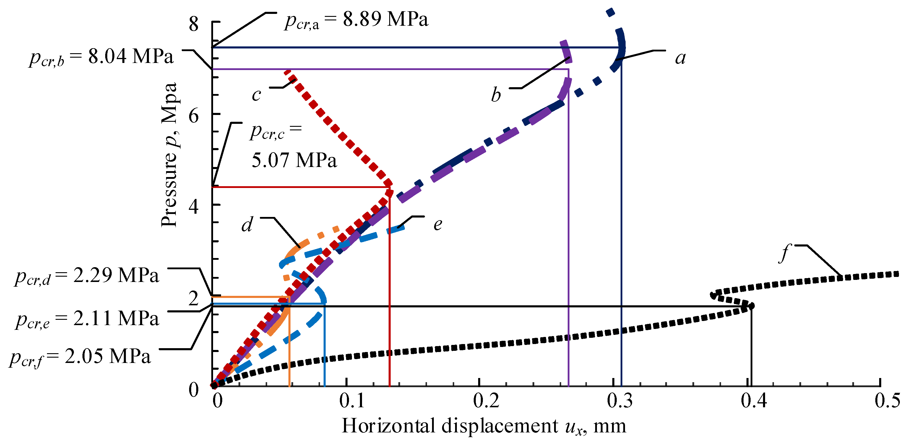
3.4. Influence of Vertebra Cortical Shell Buckling

Mechanical properties. Different properties are assigned for particular phases. The dense cortical shell phase is characterised by volume density ρ c o r = 1850 kg / m 3 [37,38], while the density of fully degenerated cancellous bone is ρ c a n = 100 kg / m 3 . The cortical phase is modelled as an isotropic elastic-plastic continuum. The elastic properties are defined by elasticity modulus E c o r = 8.0 GPa , and the Poisson’s ratio is ν c o r = 0.3 [14,39]. The plastic properties are defined on the basis of perfect plasticity and obey the von Mises yield criteria. The yield stress is σ Y = 64 MPa [14]. This value is further used as the ultimate strength constant. The trabecular phase is modelled as an elastic orthotropic continuum. The elastic modulus of the trabecular bone in the vertical (longitudinal) direction is calculated according to the formula given in Reference [40] as follows:
E c a n , z z = 4.73 ρ c a n 1.56
Thereby, the transverse elastic modulus is assumed to be the fraction of the longitudinal modulus, thus
E c a n , x x = E c a n , y y = 0.1 E c a n , z z
The Poisson’s ratio is ν c a n , x y = 0.3 , and ν c a n , x z = ν c a n , y z = 0.2 .
Finite element method. The thin-walled domain of the cortical shell was discretised by shell finite elements. The shell element applied is a four-node element with six degrees of freedom at each node. Such an element is associated with plasticity and larger strain and describes structure buckling. It is suitable for analysing thin to moderately thick shell structures. The finite element mesh of cortical shells contains 3094 nodes and 2976 shell elements.
A cancellous bone, endplates, and posterior bone models were meshed with volumetric finite elements. This type of solid element is a higher-order 3-D 20-node solid element that allows quadratic displacement behaviour. The element supports plasticity, large deflection, and large strain capabilities. Finally, the solid phase was described by a 3-D mesh containing 348,138 nodes and 147,814 solid elements. The meshed model is presented in Figure 10a.
Shell and volumetric domains may be connected in a different manner, and two computational finite element models were finally generated. The first model reflects a healthy cortex state. A connection between the cortical wall and trabecular phase is implemented as a contact of two solids (Figure 10b). In the perfect case, the connection is modelled as a bonded contact, where no sliding or separation between faces or edges is allowed. For the shell-solid constraint option, an internal set of force-distributed constraints between nodes on the shell edges and nodes on the solid surface is created. In the model, each shell node acts as the master node and associated solid nodes act as slave nodes.
In the case of osteoporotic degradation, the bond is weakened. The second model reflects the limit case with a fully degenerated interface. The degradation effect could be evaluated by removing the connecting bond, and the gap was imposed between the shell and the solid (Figure 10c). Therewithin, integrity of the body was held by connecting the edge of the shell by endplates.
Numerical results. The physical nature of different models is qualitatively illustrated by deformed shapes, and a colour plot of the displacement magnitude of the cortical shell is shown in Figure 11. The displacement values, defined in millimetres, are illustrated in a unified colour scale. The first line of subfigures (Figure 11a–c) illustrates bonded shell-solid contact, while the next line of subfigures (Figure 11d–f) illustrates unbonded contact. The first column (Figure 11a,d) reflects results obtained with the large thickness equal to 0.5 mm, while the third column (Figure 11c,f) reflects results for most degradation of cortical shell. Characterising deformation shapes in a colour scale clearly illustrates the degradation degree. Unbonded contact leads to the occurrence of two higher-order deformation modes. Extremely high displacement, which exceeds nominal values by more than 1.5 times, is observed in the vicinity of point B. This result indicates buckling of the shell in the vicinity of this point.
The most important results of the mechanical analyses are illustrated by considering the relative variation of vertebrae height h, %. According to medical practice [41], this parameter is used as a deformity grade. It is used as a fracture risk indicator. The normal state of vertebrae is characterised by deformability grade 0 which corresponds to variation 0 h 20 %. It is worth noting that the obtained values of h = 1.26 3 % are below the threshold value. The h threshold is 20%. Furthermore, the first bifurcation points of investigated vertebrae cortical shell is approximately twice higher than the maximum external loads applied in the proposed model (Figure 12). Therefore, it is obvious that buckling can be avoided in the current fracture risk model.

3.5. Discussion on Model Limitations

Creep. The deformations of bone under the load are time dependent not only due to osteoporosis but also due to creep [42,43,44]. Therefore, the long-term critical force or long-term strength of the bone is less than the short-term critical force or short-term strength. In case of the long-term deformation, long term deformation of the bone subject to long-term loading can be modelled properly using well-developed viscoelasticity or creep theories developed in the mechanics of materials provided that the characteristics of the bone is known, for example, modulus of elasticity, compliance function, or creep function. However, in the case of osteoporosis, the common viscoelasticity theories are not suitable due to fact that, in the classic viscoelasticity theories, the derivatives of the modulus of elasticity and the creep functions with respect to the time are nonnegative. In other words, the modulus of elasticity is a non-decreasing function with respect to time. However, in the case of osteoporosis, these conditions are violated and the long term analysis of the bone deformations when the osteoporosis simultaneously takes place is a much more complicated problem that also demands profound theoretical reconsiderations of the existing creep or viscoelasticity theories. The raised issue demands separate profound investigations which is not possible in the present study.
Anisotropy. Trabeculae bone tissues are strongly anisotropic materials with individual mechanical and topological properties for each patient. Good known representative volume elements (RVE) and homogenization-based methods [45] require topology of trabeculae, which needs micro-CT or micro-MRI scans. In the case of lumbar vertebra, they are impossible or very expansive. Therefore, modelling of mechanical behaviour of patient-specific lumbar vertebra is the challenge and we needs some indirect methods for evaluating mechanical properties of patient-specific lumbar veretbra trabeculae. Wolf’s law [46] helps to understand the anisotropy of mechanical properties of bone, and from theoretical point of view, we can still investigate simplified trabecular structures arranged in the direction of external stresses as a suitable mechanical model if we want to understand mechanical behaviour of trabeculae inside a vertebral body. On the other hand, it is experimentally observed fact that, in vertebra L1, trabeculae arrangement is remodelled to withstand maximal compression loads. So, choosing of numerical compression tests is logical too.
Yield criteria. In general, lumbar vertebrae are strongly anisotropic plastic biological tissue. Therefore, failure criteria should be based on yield surface, which can be expressed as a Taylor expansion [47]
i k a i k σ i k α + p q m n a p q m n σ p q σ m n β + r s t l m n a r s t l m n σ r s σ t l σ m n γ 1
where a i k , a p q m n , a r s t l m n are strength tensors of different order. von Mises [48] proposed yield criterion for isotropic materials. Hill [49] extended the von Mises yield criterion of isotropic materials to anisotropic materials. Later Tsai [50] extended this criterion for anisotropic materials to a unidirectional lamina. It is easy to show that von Mises or Tsai–Hill failure criteria can be derived form Goldenblar–Kopnov failure criteria. Two-dimensional failure propagation simulations by Korenczuk et al. [51] showed that the von Mises failure criterion did not capture the failure type, location, or propagation direction nearly as well as the Tsai–Hill criterion. Both the von Mises and Tsai–Hill failure criteria severely underpredicted the amount of displacement needed to produce initial failure in the porcine abdominal aortas. Therefore, using of von Mises or Tsai–Hill failure criteria would overestimate lumbar vertebra fracture risk.
Remodelling. One-time resonant destruction of vertebra is a very rare clinical dysfunction, which was not investigated in our model. On the other hand, according to Wolf’s low, long range loads enable the increase of bone strength in the greatest load direction and opposite decrease strength in lowest load direction. Therefore, we would take into account additionally bone remodelling or its fatigue property, but this article does not include an investigation of vertebra remodelling.

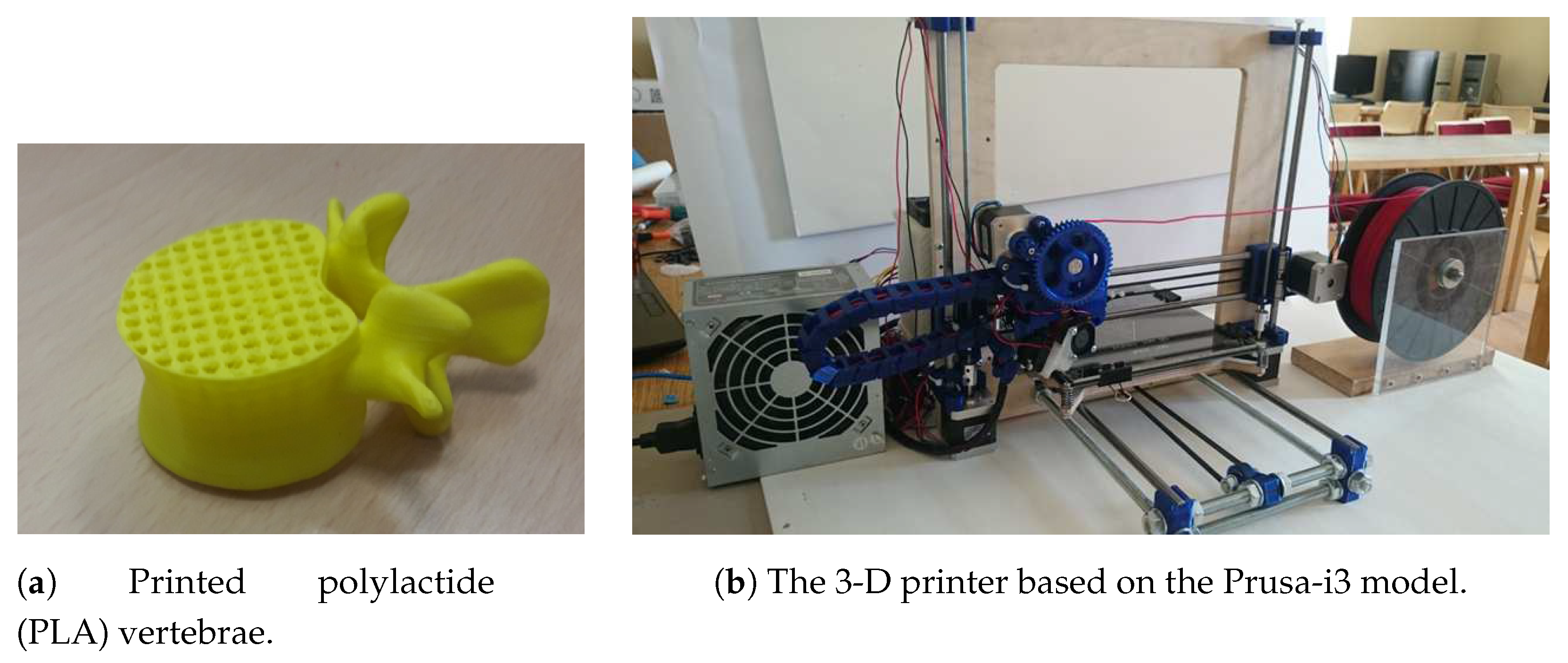
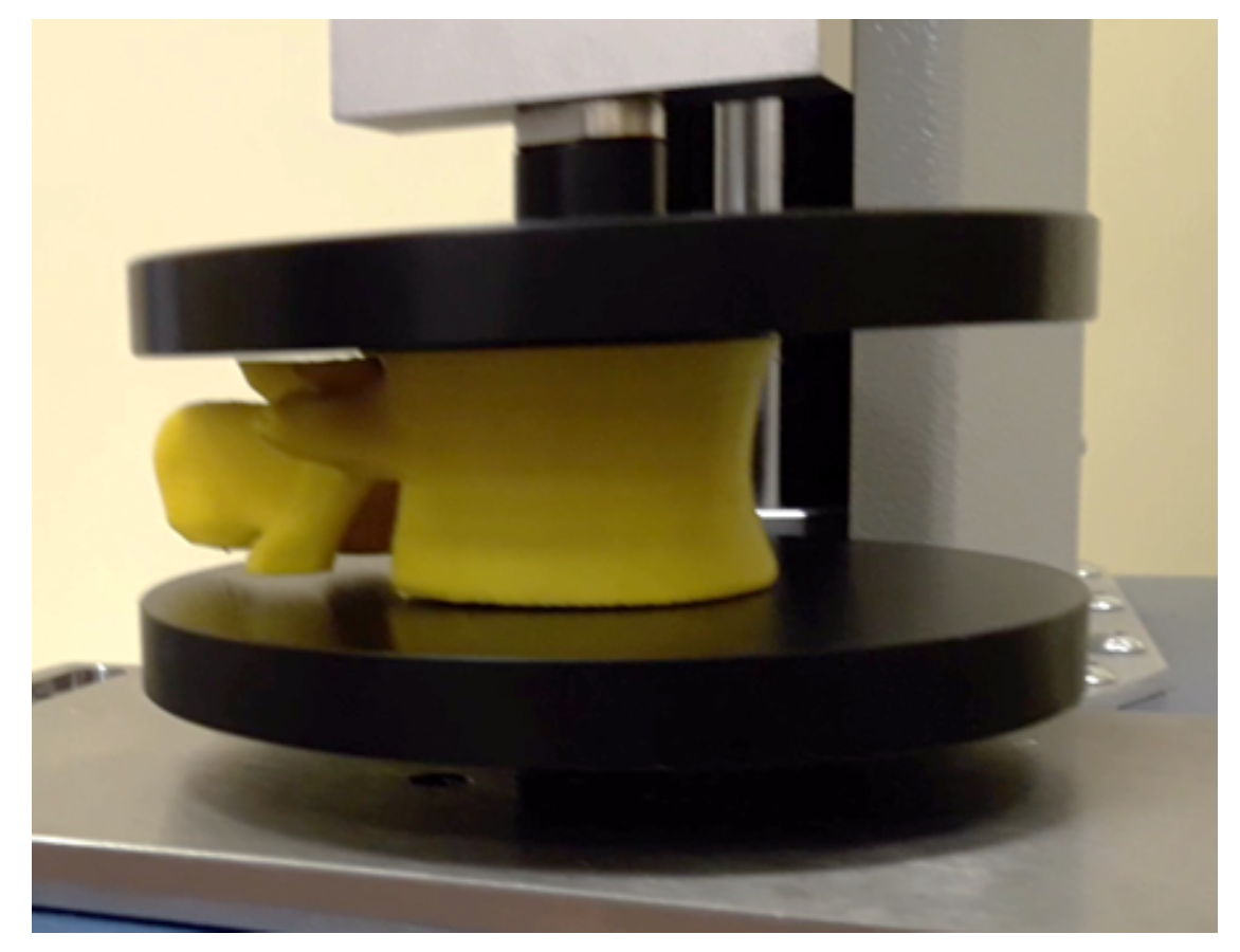
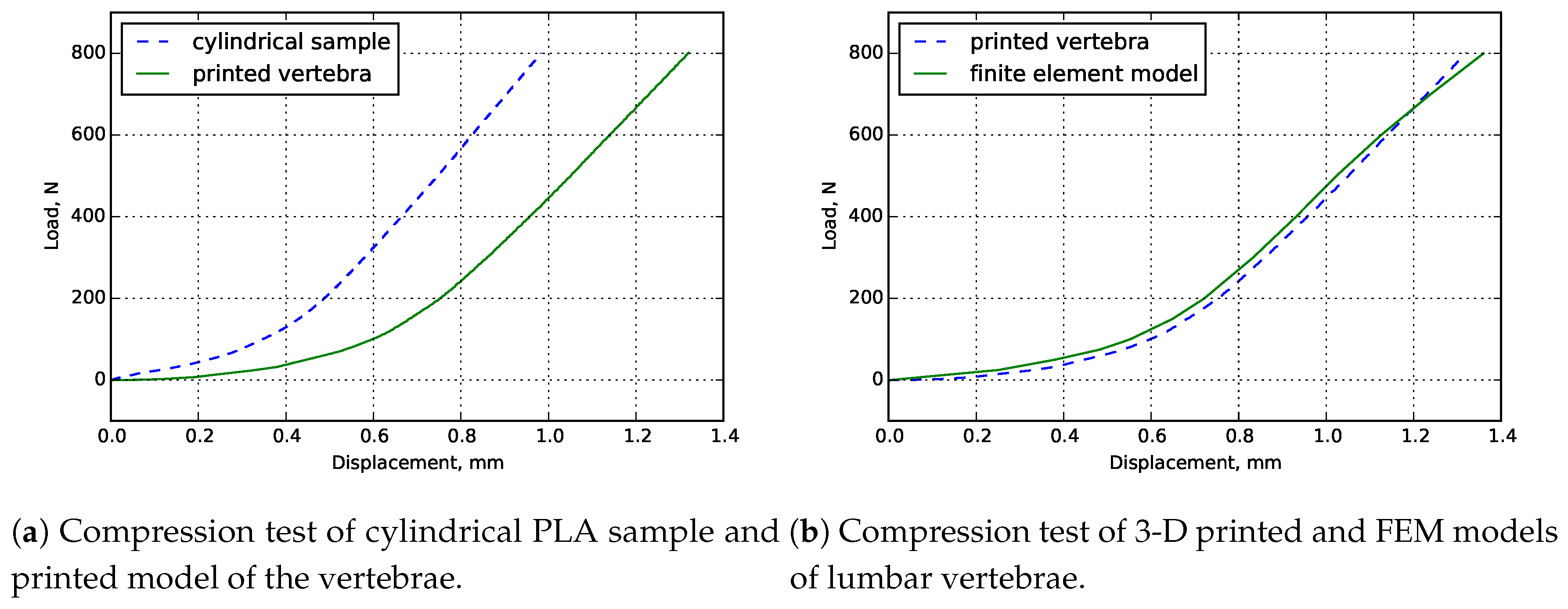
3.6. Validation of Mechanical Model

Extracting physical and micro-geometrical properties of vertebrae is very complicated. If we want to know micro-geometry of human bones, quantitative computational tomography (QCT) can be used on leg or hand bones but not on whole human spine or one of vertebra. Therefore, an alternating methodology of investigation of vertebrae mechanical properties can be 3-D printing. As is stated in Reference [52], today, 3-D printing is practical, useful technology in surgical planing or spine implantation. Obviously, knowing mechanical characteristics, 3-D printed vertebrae is the basic step in successful applications of such kind of structures.
The validation of numerical modelling was aided in our case by a physical test of the printed polylactide (PLA) vertebrae geometrical model (Figure 13a). The whole procedure took the following the steps:
  • The printing of the vertebrae model;
  • The printing of the cylindrical PLA sample for mechanical properties of PLA to define;
  • The compression test of the printed PLA sample;
  • The compression test of the printed PLA vertebrae;
  • The determination of the mechanical properties of PLA by verifying the obtained load-displacement curve of the cylindrical sample;
  • The implementation of the defined stress-strain curve of PLA onto the numerical calculation;
  • The comparison of the results of the experimental and numerical studies.
The printing process was realized by using self-made 3-D printer, based on Prusa-i3 model (Figure 13b). The selection of this device was justified by its parameters: printer type FDM, build volume, 25 × 21 × 20 cm 3 , minimal layer height 50 μ m, and nozzle diameter 0.2 mm. The printing process took about 20 h, while the printing was completed. The properties of the osteoporotic sample of vertebrae was as follow: thickness of cortical shell, 0.5 mm, 0.1 BV/TV ratio, and 1.2 TBS.
The physical experiment was performed by using a MultiTest 2.5-i compression machine (Figure 14). The selection of this device was based on suitable range of load 0–2500 N and relatively high precision ( ± 0.1 % of full scale). The sample vertebra was tested under the constant loading speed (10 mm/min), and the displacement values were obtained: They are presented in Figure 15a. The same test was accomplished for the printed cylindrical sample too.
As Figure 15a shows, the nonlinear behaviour of the printed PLA was revealed. The mechanical properties of PLA were determined by processing the load-displacement curve of the cylindrical sample (20 mm length, 15 mm diameter), and the stress–strain relation of PLA was defined.
The defined stress–strain curve of PLA (Figure 15a) was integrated into the numerical model of the vertebrae, and the finite element study was compared to the results of the physical experiment (Figure 15b).
As Figure 15b shows, the curves present corresponding characters, and the biggest difference between the results is constant (about 4%) until the value of load becomes 700 N. Then, the curves demonstrate similar magnitudes of displacement values, which does not exceed 5%. These results approve the adequacy of finite element model and shows that the method offered for osteoporotic bone validation is reliable.

4. Conclusions

The proposed method based on the cancellous bone and cortical shell in silico finite element modelling includes basic principles of evaluating fracture risk of the mechanical system and can be used after clinical researches to estimate the quantiles of the load-bearing capacity of a lumbar vertebra as well as the fracture risk of individual patients by applying the peculiar anatomical properties of the lumbar vertebra.
The results show that the fracture risk is substantially higher at relatively low levels of apparent BV/TV ratios and critical due to thinner cortical shells, suggesting high risk levels even during daily activities of typical external loads.

Author Contributions

Conceptualization, A.M., V.A., M.T. and R.K.; data curation, A.M., O.A. and O.C.; formal analysis, A.M. and D.Z.; funding acquisition, A.M.; investigation, A.M., O.A., O.C. and D.Z.; methodology, A.M., D.Z. and R.K.; project administration, A.M.; resources, A.M.; software, A.M. and D.Z.; supervision, A.M.; validation, A.M., O.A., O.C. and D.Z.; visualization, O.A., O.C. and D.Z.; writing—original draft, A.M., V.A., D.Z. and M.T.; writing—review and editing, A.M., V.A., D.Z. and M.T.

Funding

This research received no external funding.

Conflicts of Interest

The authors declare no conflict of interest.

Abbreviations

The following abbreviations are used in this manuscript:
FEMFinite element method
FEFinite element
IVDintervetebral disk
BV/TVBone volume vs total volume
QCTQuantitative computational tomography
BMDBone mineral density
DXADual-energy X-ray absorptiometry

References

  1. Agrawal, A.; Kalia, R. Osteoporosis: Current Review. J. Orthop. Traumatol. Rehabil. 2014, 7, 101. [Google Scholar] [CrossRef]
  2. Lin, J.T.; Lane, J.M. Osteoporosis: A review. Clin. Orthop. Relat. Res. 2004, 425, 126–134. [Google Scholar] [CrossRef]
  3. Cooper, C.; Cole, Z.A.; Holroyd, C.R.; Earl, S.C.; Harvey, N.C.; Dennison, E.M.; Melton, L.J.; Cummings, S.R.; Kanis, J.A. The IOF CSA Working Group on Fracture Epidemiology. Secular trends in the incidence of hip and other osteoporotic fractures. Osteoporos. Int. 2011, 22, 1277–1288. [Google Scholar] [CrossRef]
  4. Cummings, S.R.; Melton, L.J., III. Epidemiology and outcomes of osteoporotic fractures. Lancet 2002, 359, 1761–1767. [Google Scholar] [CrossRef]
  5. Doblaré, M.; García, J.M.; Gómez, M.J. Modelling bone tissue fracture and healing: A review. Eng. Fract. Mech. 2004, 71, 1809–1840. [Google Scholar] [CrossRef]
  6. odygowski, T.; Kakol, W.; Wierszycki, M.; Ogurkowska, B.M. Three-dimensional nonlinear finite element model of the human lumbar spine segment. Acta Bioeng. Biomech. 2005, 7, 17–28. [Google Scholar]
  7. Su, J.; Cao, L.; Li, Z.; Yu, B.; Zhang, C.; Li, M. Three-dimensional finite element analysis of lumbar vertebra loaded by static stress and its biomechanical significance. Chin. J. Traumatol. 2009, 12, 153–156. [Google Scholar]
  8. Jones, A.C.; Wilcox, R.K. Finite element analysis of the spine: Towards a framework of verification, validation and sensitivity analysis. Med. Eng. Phys. 2008, 30, 1287–1304. [Google Scholar] [CrossRef]
  9. Crawford, R.P.; Cann, C.E.; Keaveny, T.M. Finite element models predict in vitro vertebral body compressive strength better than quantitative computed tomography. Bone 2003, 33, 744–750. [Google Scholar] [CrossRef]
  10. Maquer, G.; Schwiedrzik, J.; Huber, G.; Morlock, M.M.; Zysset, P.K. Compressive strength of elderly vertebrae is reduced by disc degeneration and additional flexion. J. Mech. Behav. Biomed. Mater. 2015, 42, 54–66. [Google Scholar] [CrossRef] [Green Version]
  11. Provatidis, C.; Vossou, C.; Koukoulis, I.; Balanika, A.; Baltas, C.; Lyritis, G. A pilot finite element study of an osteoporotic L1-vertebra compared to one with normal T-score. Comput. Methods Biomech. Biomed. Eng. 2010, 13, 185–195. [Google Scholar] [CrossRef]
  12. McDonald, K.; Little, J.; Pearcy, M.; Adam, C. Development of a multi-scale finite element model of the osteoporotic lumbar vertebral body for the investigation of apparent level vertebra mechanics and micro-level trabecular mechanics. Med. Eng. Phys. 2010, 32, 653–661. [Google Scholar] [CrossRef] [Green Version]
  13. Garo, A.; Arnoux, P.J.; Wagnac, E.; Aubin, C.E. Calibration of the mechanical properties in a finite element model of a lumbar vertebra under dynamic compression up to failure. Med. Biol. Eng. Comput. 2011, 49, 1371–1379. [Google Scholar] [CrossRef]
  14. Kim, Y.H.; Wu, M.; Kim, K. Stress Analysis of Osteoporotic Lumbar Vertebra Using Finite Element Model with Microscaled Beam-Shell Trabecular-Cortical Structure. J. Appl. Math. 2013, 2013, 285165. [Google Scholar] [CrossRef]
  15. Wierszycki, M.; Szajek, K.; Łodygowski, T.; Nowak, M. A two-scale approach for trabecular bone microstructure modeling based on computational homogenization procedure. Comput. Mech. 2014, 54, 287–298. [Google Scholar] [CrossRef] [Green Version]
  16. Wolfram, U.; Gross, T.; Pahr, D.H.; Schwiedrzik, J.; Wilke, H.J.; Zysset, P.K. Fabric-based Tsai-Wu yield criteria for vertebral trabecular bone in stress and strain space. J. Mech. Behav. Biomed. Mater. 2012, 15, 218–228. [Google Scholar] [CrossRef]
  17. El-Rich, M.; Arnoux, P.J.; Wagnac, E.; Brunet, C.; Aubin, C.E. Finite element investigation of the loading rate effect on the spinal load-sharing changes under impact conditions. J. Biomech. 2009, 42, 1252–1262. [Google Scholar] [CrossRef]
  18. Pothuaud, L.; Carceller, P.; Hans, D. Correlations between grey-level variations in 2D projection images (TBS) and 3D microarchitecture: Applications in the study of human trabecular bone microarchitecture. Bone 2008, 42, 775–778. [Google Scholar] [CrossRef]
  19. Hans, D.; Barthe, N.; Boutroy, S.; Pothuaud, L.; Winzenrieth, R.; Krieg, M.-A. Correlations Between Trabecular Bone Score, Measured Using Anteroposterior Dual-Energy X-Ray Absorptiometry Acquisition, and 3-Dimensional Parameters of Bone Microarchitecture: An Experimental Study on Human Cadaver Vertebrae. J. Clin. Densitom. 2011, 14, 302–312. [Google Scholar] [CrossRef]
  20. Kanis, J.A.; Oden, V.; Johnell, O.; Johansson, H.; De Laet, C.; Brown, J.; Burckhardt, P.; Cooper, C.; Christiansen, C.; Cummings, S.; et al. The use of clinical risk factors enhances the performance of BMD in the prediction of hip and osteoporotic fractures in men and women. Osteoporos. Int. 2007, 18, 1033–1046. [Google Scholar] [CrossRef]
  21. Marshall, D.; Johnell, O.; Wedel, H. Meta-analysis of how well measures of bone mineral density predict occurrence of osteoporotic fractures. BMJ 1996, 312, 1254–1259. [Google Scholar] [CrossRef] [Green Version]
  22. Taylor, B.C.; Schreiner, P.J.; Stone, K.L.; Fink, H.A.; Cummings, S.R.; Nevitt, M.C.; Bowman, P.J.; Ensrud, K.E. Long-term prediction of incident hip fracture risk in elderly white women: Study of osteoporotic fractures. J. Am. Geriatr. Soc. 2004, 52, 1479–1486. [Google Scholar] [CrossRef]
  23. Kanis, J.A.; Oden, A.; Johansson, H.; Borgstrom, F.; Strom, O.; McCloskey, E. FRAX and its applications to clinical practice. Bone 2009, 44, 734–743. [Google Scholar] [CrossRef]
  24. Kanis, J.A.; Johnell, O.; Oden, A.; Johansson, H.; McCloskey, E. FRAX and the assessment of fracture probability in men and women from the UK. Osteoporos. Int. 2008, 19, 385–397. [Google Scholar] [CrossRef]
  25. Timothy, H.K.; Brandeau, J.F. Mathematical modeling of the stress strain-strain rate behavior of bone using the Ramberg-Osgood equation. J. Biomech. 1983, 16, 445–450. [Google Scholar]
  26. Nazarian, A.; von Stechow, D.; Zurakowski, D.; Muller, R.; Snyder, B.D. Bone Volume Fraction Explains the Variation in Strength and Stiffness of Cancellous Bone Affected by Metastatic Cancer and Osteoporosis. Calcif. Tissue Int. 2008, 83, 368–379. [Google Scholar] [CrossRef]
  27. Abaqus FEA, SIMULIA Web Site. Dassault Systèmes, Retrieved 2017. Available online: https://www.3ds.com/ (accessed on 25 July 2019).
  28. Linthorne, N.P. Analysis of standing vertical jumps using a force platform. J. Sports Sci. Med. 2010, 9, 282–287. [Google Scholar] [CrossRef]
  29. Dodson, B.; Noland, D. Reliability Engineering Handbook; CRC Press LLC Main Office: Boca Raton, FL, USA, 1999; p. 592. [Google Scholar]
  30. Melton, L.J., III; Achenbach, S.J.; Atkinson, E.J.; Therneau, T.M.; Amin, S. Long-term mortality following fractures at different skeletai sites: A population-based cohort study. Osteoporos. Int. 2013, 24, 1689–1696. [Google Scholar] [CrossRef]
  31. R Core Team. R: A Language and Environment for Statistical Computing; R Foundation for Statistical Computing: Vienna, Austria, 2017; Available online: https://www.R-project.org/ (accessed on 25 July 2019).
  32. Pinheiro, J.; Bates, D.; DebRoy, S.; Sarkar, D.; R Core Team (2017). Nlme: Linear and Nonlinear Mixed Effects Models. R Package Version 3.1-131. 2017. Available online: https://CRAN.R-project.org/package=nlme (accessed on 25 July 2019).
  33. Fields, A.J.; Eswaran, S.K.; Jekir, M.G.; Keaveny, T.M. Role of trabecular microarchitecture in whole-vertebral body biomechanical behavior. J. Bone Miner. Res. 2009, 24, 1523–1530. [Google Scholar] [CrossRef]
  34. Roux, J.P.; Wegrzyn, J.; Arlot, M.E.; Guyen, O.; Delmas, P.D.; Chapurlat, R.; Bouxsein, M.L. Contribution of trabecular and cortical components to biomechanical behavior of human vertebrae: An ex vivo study. J. Bone Miner. Res. 2010, 25, 356–361. [Google Scholar] [CrossRef]
  35. Jaumard, N.V.; Bauman, J.A.; Weisshaar, C.L.; Guarino, B.B.; Welch, W.C.; Winkelstein, B.A. Contact pressure in the facet joint during sagittal bending of the cadaveric cervical spine. J. Biomech. Eng. 2011, 133, 071004. [Google Scholar] [CrossRef]
  36. Venables, W.N.; Ripley, B.D. Modern Applied Statistics with S, 4th ed.; Springer: New York, NY, USA, 2002; ISBN 0-387-95457-0. [Google Scholar]
  37. Mann, K.A.; Miller, M.A. Fluid-structure interactions in micro-interlocked regions of the cement-bone interface. Comput. Methods Biomech. Biomed. Eng. 2014, 17, 1809–1820. [Google Scholar] [CrossRef]
  38. Souzanchi, M.F.; Palacio-Mancheno, P.; Borisov, Y.A.; Cardoso, L.; Cowin, S.C. Microarchitecture and bone quality in the human calcaneus: Local variations of fabric anisotropy. J. Bone Min. Res. 2012, 27, 2562–2572. [Google Scholar] [CrossRef] [Green Version]
  39. Polikeit, A.; Nolte, L.P.; Ferguson, S.J. Simulated influence of osteoporosis and disc degeneration on the load transfer in a lumbar functional spinal unit. J. Biomech. 2004, 37, 1061–1069. [Google Scholar] [CrossRef]
  40. Helgason, B.; Perilli, E.; Schileo, E.; Taddei, F.; Brynjólfsson, S.S.; Viceconti, M. Mathematical relationships between bone density and mechanical properties: A literature review. Clin. Biomech. 2008, 23, 135–146. [Google Scholar] [CrossRef]
  41. Genant, H.K.; Wu, C.Y.; van Kuijk, C.; Nevitt, M.C. Vertebral fracture assessment using a semiquantitative technique. J. Bone Min. Res. 1993, 8, 1137–1148. [Google Scholar] [CrossRef]
  42. Lakes, R.S.; Katz, J.L.; Sternstein, S.S. Viscoelastic properties of wet cortical bone: Part I, torsional and biaxial studies. J. Biomech. 1979, 12, 657–678. [Google Scholar] [CrossRef]
  43. Lakes, R.S.; Katz, J.L. Viscoelastic properties of wet cortical bone: Part II, relaxation mechanisms. J. Biomech. 1979, 12, 679–687. [Google Scholar] [CrossRef]
  44. Lakes, R.S.; Katz, J.L. Viscoelastic properties of wet cortical bone: Part III, A non-linear constitutive equation. J. Biomech. 1979, 12, 689–698. [Google Scholar] [CrossRef]
  45. Burczinski, T. Multiscale Modelling of Osseous Tissues. J. Theor. Appl. Mech. 2010, 48, 855–870. [Google Scholar]
  46. Wolf, J. Das Gesetz der Transformation der Knochen; Hirschwald: Berlin, Germany, 1892. [Google Scholar]
  47. Goldenblar, I.I.; Kopnov, A. Strength of Glass Reinforced Plastics in the Complex Stress State. Polym. Mech. 1966, 1, 54–60. [Google Scholar] [CrossRef]
  48. von Mises, R. Mechanik der festen Körper im plastisch deformablen Zustand Göttin. Nachr. Math. Phys. 1913, 1, 582–592. [Google Scholar]
  49. Hill, R. The Mathematical Theory of Plasticity; Oxford, U.P.: Oxford, UK, 1950. [Google Scholar]
  50. Tsai, S.W. Strength Theories of Filamentary Structures. In Fundamental Aspects of Fibre Reinforced Plastic Composites; Schwartz, R.T., Schwartz, H.S., Eds.; Interscience: New York, NY, USA, Chapter 1; 1968. [Google Scholar]
  51. Korenczuk, C.E.; Votava, L.E.; Dhume, R.Y.; Kizilski, S.B.; Brown, G.E.; Narain, R.; Barocas, V.H. Isotropic Failure Criteria Are Not Appropriate for Anisotropic Fibrous Biological Tissues. J. Biomech. Eng. 2017, 139, 071008. [Google Scholar] [CrossRef]
  52. Wilcox, B.; Mobbs, R.J.; Wu, A.M.; Phan, K. Systematic review of 3D printing in spinal surgery: The current state of play. J. Spine Surg. 2017, 3, 433–443. [Google Scholar] [CrossRef]
Figure 1. Geometrical models of vertebra.
Applsci 09 03013 g001
Figure 2. Osgood–Ramberg stress–strain relation for cortical bone.
Applsci 09 03013 g002
Figure 3. Load conditions of the compression test.
Applsci 09 03013 g003
Figure 4. Time curve of dynamic load.
Applsci 09 03013 g004
Figure 5. Results of the static analysis.
Applsci 09 03013 g005aApplsci 09 03013 g005b
Figure 6. Results of the dynamic analysis.
Applsci 09 03013 g006aApplsci 09 03013 g006b
Figure 7. Relative residuals versus calculated values of the maximum von Mises stress.
Applsci 09 03013 g007
Figure 8. Realizations of the probability density functions of the random variables X β (a,d); r.v. X δ (b,e); and r.v. Y p , R (c,f). Density function realizations of initial independent variables
Applsci 09 03013 g008
Figure 9. Realizations of the probability density functions of the random variables X p , E and Y p , R (a) for Case I and (c) for Case II; and empirical cumulative distribution functions F ^ Z , i ( z ) of r.v. Z = Y p , E X p , E and failure risks P r f , i , i { 1 , 2 , 3 } for Case I (b) and for Case II (d): F ^ Z , 1 ( z ) and p r f , 1 when M ( G p , E ) = p m i n ; F ^ Z , 2 ( z ) and p r f , 2 when M ( G p , E ) = 1.5 p m i n ; F ^ Z , 3 ( z ) and p r f , 3 when M ( G p , E ) = 2.5 p m i n , where correlation coefficient C v a r ( G p , E ) = 0.2 for all P r f , i , F ^ Z , i ( z ) , i { 1 , 2 , 3 } .
Applsci 09 03013 g009
Figure 10. Cross-sectional view of the 3-D finite element model of the vertebra in the sagittal plane (a); bonded and unbonded, with a gap and cortical shells (b,c) respectively.
Applsci 09 03013 g010
Figure 11. Deformed shape effect at the first bifurcation point A. Figure a–c for the bonded trabecular bone (Figure 10b): (a) when δ = 0.5 , t = 0.86 t m a x , (b) when δ = 0.4 mm and t = 0.85 t m a x , (c) when δ = 0.2 mm and t = 0.58 t m a x . Figure d–f for the unbounded trabecular bone (Figure 10c): (d) when δ = 0.5 mm and t = 0.32 t m a x , (e) when δ = 0.4 mm and t = 0.32 t m a x , (f) when δ = 0.2 mm and t = 0.38 t m a x .
Applsci 09 03013 g011
Figure 12. Load dependency graph. Displacement in horizontal direction at point A (Figure 11).
Applsci 09 03013 g012
Figure 13. The 3-D printer and printed vertebra.
Applsci 09 03013 g013
Figure 14. Testing of printed vertebrae by the compression machine.
Applsci 09 03013 g014
Figure 15. The load-displacement curves.
Applsci 09 03013 g015
Table 1. Elasticity constants of model components.
PropertyLumbar BodyIntervertebra Disc
Young modulus, MPa800010
Ulimate strength, MPa60-
Yield strength, MPa40-
Poisson’s ratio0.300.40
Table 2. The parameters of a healthy and osteoporotic model.
ModelThickness, mmBV/TVTBS
Healthy0.50.351.45
Ostseopenea0.40.201.33
Osteoporosis0.20.101.20
Table 3. The parameters of different lumbar body models.
Cortical Shell Thickness, mmBV/TVTBS
0.200.101.28
0.400.101.28
0.500.101.28
0.200.201.33
0.400.201.33
0.500.201.33
0.200.351.45
0.400.351.45
0.500.351.45
Table 4. The maximum von Mises stresses of the static analysis calculated by finite element method (FEM) at different δ β , and p
AnalysisThickness, mm, δ BV/TV, β External Load, MPa, p
0.150.300.450.600.75
Static0.50.102.96.19.312.315.2
0.202.04.16.18.28.5
0.351.63.45.06.78.5
0.40.103.46.710.214.117.0
0.202.14.26.38.410.5
0.351.83.55.47.39.1
0.20.1018.924.131.340.849.4
0.2013.318.423.228.133.5
0.3512.117.421.024.528.0

