Hierarchical Guided-Image-Filtering for Efficient Stereo Matching

Featured Application

Potential applications of the work include autonomous navigation, 3D reconstruction, and vision-based object handling.

Abstract

Stereo matching is complicated by the uneven distribution of textures on the image pairs. We address this problem by applying the edge-preserving guided-Image-filtering (GIF) at different resolutions. In contrast to most multi-scale stereo matching algorithms, parameters of the proposed hierarchical GIF model are in an innovative weighted-combination scheme to generate an improved matching cost volume. Our method draws its strength from exploiting texture in various resolution levels and performing an effective mixture of the derived parameters. This novel approach advances our recently proposed algorithm, the pervasive guided-image-filtering scheme, by equipping it with hierarchical filtering modules, leading to disparity images with more details. The approach ensures as many different-scale patterns as possible to be involved in the cost aggregation and hence improves matching accuracy. The experimental results show that the proposed scheme achieves the best matching accuracy when compared with six well-recognized cutting-edge algorithms using version 3 of the Middlebury stereo evaluation data sets.

1. Introduction

Stereo vision aims at providing rich distance information of the captured scenes via image pairs. This is normally accomplished by matching algorithms to generate dense disparity maps. The maps can be transformed into three-dimensional information of the scene by the principle of triangulation with many potential applications, such as autonomous navigation, 3D reconstruction, and vision-based object handling.

Although the stereo matching problem has been under extensive research for decades, it is still difficult to obtain accurate matching under ill-posed conditions such as texture-less regions, repeated patterns, occlusion areas, and reflective surfaces. The current stereo matching algorithms can mainly be divided into two categories: The conventional matching algorithms [1] and the deep-learning-based stereo matching approaches.

The stereo matching algorithm based on deep learning regards the process of deriving the disparity map as a classification problem or a regression problem. For instance, Zbontar [2] used the convolutional neural networks (CNNs) to estimate the similarity of image blocks and uses the measures as the matching cost in the traditional stereo matching algorithm. Similarly, Nahar [3] proposed unsupervised pre-trained networks to estimate hierarchical features and combine them with a pixel-based intensity matching cost in a global energy minimization framework for dense disparity estimation. By combining a disparity estimation network with a CNN that was trained by a synthetically generated dataset, Mayer [4] demonstrated the effectiveness of deep learning in stereo matching. Pang [5] proposed a cascaded CNN architecture that is composed of two stages: The first stage advances the work of Reference [4] by equipping it with extra up-convolution modules, while the second stage generates residual signals across multiple scales. The summation of the outputs from the two stages gives the final disparity. Kendall [6] used deep unary features to compute a stereo matching cost volume. In this approach, disparity values are regressed for aggregation from the cost volume using 3D convolutions.

Another method to implement deep learning-based stereo matching is to use the networks to exploit context information. For example, Chang [7] developed a spatial pyramid pooling module to the aggregate context in different scales to form a cost volume. The cost volume is regularized by a stacked network to further improve the utilization of global context information. Besides, Williem [8] used the deep learning technique for the cost volume aggregation based on self-guided filtering.

Deep learning-based methods are promising as they can apply the high-level object detection as a guideline for within-object matching. However, most of the current schemes use supervised learning methods that assume the true disparity is known in advance. This assumption is impractical for many applications [9]. Moreover, these approaches might be invalid for an unknown environment and cannot be well transplanted to robotic and embedded systems [10].

The conventional stereo matching approaches are classified as global or local according to the construction of an objective function that rates the degree of match between an image pair [1]. The objective function of the global methods consists of a data term (the measurement part) and a regularization term (the penalty part). The data term designates the similarity between aggregated matching costs of pixels on the images, and the regularization term is included to provide constraints from neighboring pixels. Belief propagation [11] and dynamic programming [12,13] are the major global methods. However, global approaches need a lot of computing resource and are generally not suitable for real-time applications.

In contrast to the global approaches, the objective function of the local methods contains only the measurement part. The local methods generally perform the stereo matching in four stages [1]: (1) The calculation of the preliminary matching cost, (2) aggregation of the cost over support windows, (3) estimation of the disparity, and (4) refining the disparity. Among them, the cost aggregation step is usually transformed into an image filtering procedure of the matching cost and the disparity maps are obtained by the winner-takes-all method [1]. The local methods require less computation and are popular for fast disparity calculations.

Cost aggregation is crucial for matching performance in the local algorithms. Bilateral filtering [14] is among the early approaches that led to the increase of computational complexity with the increase of support-window size. Later, tree filtering [15], domain transformation [16], recursive edge-aware filter [17], and full-image guided filtering [18] were proposed to decouple computational complexity with the support window size. However, these approaches all suffer from the weight-decay problem when there is a significant intensity difference between neighboring pixels. This behavior deteriorates information propagation and impairs the resulting matching performance.

Hosni [19] suggested treating the generation of disparity as a labeling problem, which is implemented through the steps of constructing a cost volume, cost volume filtering, followed by winner-takes-all label selection. Along this line, the guided-image-filter (GIF) [20] substantially involves cost volume filtering because it can generate clear edge profiles free from the gradient-reversal artifacts. Later, Li [21] introduced an edge-aware weighting, denoted as the weighted guided-image-filtering (WGIF), to improve GIF. Kou [22] proposed a gradient-domain guided-image-filter (GDGIF) to reduce halo artifacts by incorporating an explicit first-order edge-aware constraint. Nevertheless, due to the lack of pixel information outside the fixed window, the implementation of WGIF by Hong [23] results in restricted performance.

To remove the fixed-window limitation, approaches with adaptive guided filters were proposed [24]. However, information outside the support windows is still missing. In a recent paper [25], we introduced weights that take both distance and intensity differences into account to extend the scheme of GIF. We called our approach the pervasive guided-image-filtering, denoted as PGIF [25], which exploits the whole image for aggregation.

Also, recent years have seen the development of coarse-to-fine (CTF) strategies to enhance the stereo matching accuracy. For instance, Hu [26] proposed to reduce the search space of local stereo matching by introducing a candidate set of neighbor pixels. Tang [27] introduced a multi-scale pixel feature vector to provide effective matching of radiometric differences. Advanced techniques to find improved disparity range was provided in the work of Li [28] by recursive multi-scale decomposition. These methods assume the existence of disparity consistency. In contrast to these approaches, the matching cost integration method of Zhang [29] resulted in superior matching, where cost aggregation is formulated to enforce the consistency of the cost volume among the neighboring scales.

Inspired by the multiscale scheme of Zhang [29], we extend the pervasive guided-image-filtering, PGIF [25], to exploit the cross-scale features in the cost volume. In our approach, the consistency is imposed on the GIF parameters, rather than the cost volume of Zhang [29], in the neighboring-scale direction. We call it hierarchical guided-image-filtering, denoted as HGIF.

The main contribution of this paper can be summarized as:

(1)

We created an innovative aggregation approach that efficiently combines the model parameters of PGIF [25] to allow the features of the image pairs in different resolutions to be considered;

(2)

The scheme is unique in its parameter-based aggregation, rather than the cost-volume-based approaches in the current literature, allowing efficient calculation with superior performance;

(3)

The proposed scheme outperforms most of the state-of-art algorithms in terms of disparity accuracy even without the refinement procedure.

2. Proposed Method

2.1. The Cost Aggregation Based on the Pervasive Guided-Image-Filtering (PGIF)

This section presents the basic procedure of the pervasive guided-image-filtering (PGIF) [25] scheme. It serves as the definitions of some of the variables and algorithms for the proposed scheme to be shown in the next section.

In the GIF-based stereo matching algorithms, such as WGIF [21], GDGIF [22], and PGIF [25] are discussed in the last section. The aggregated cost, ${\overline{C}}_{d,0}(p)$ is a linear function of the guidance image, $I_G$ at a local disparity patch such that:

$${\overline{C}}_{d,0}(p)=a_{d,0}(p)\cdot I_G(p)+b_{d,0}(p),$$

(1)

where $p=(x,y)$ is the location of the central pixel and $d$ indicates the disparity. Note that ${\overline{C}}_{d,0}(p)$ have three dimensions $(x,y,d)$ and is often denoted as the aggregated cost volume. Likewise, $a_{d,0}(p)$ and $b_{d,0}(p)$ can also be called the parameter volumes of the model. The second subscript, 0, indicates that these values are related to the original resolution. For the following stereo matching operations, we regard the left image as the reference image, such that $I_G=I_{L,0}$, and the right image as the target image.

The disparity map, $D(p)$ is composed of the disparity value corresponding to the minimum aggregated cost at each location p:

$$D(p)=\arg \underset{d}{\min }{\overline{C}}_{d,0}(p).$$

(2)

In order to solve for $a_{d,0}(p)$ and $b_{d,0}(p)$, we proposed an objective function in Reference [25], which includes a weighted sum of the squared difference between the linear model and a primary matching cost, denoted as $C_{d,0}(q)$, and a regularization term:

$$E_{d,0}(p)={\displaystyle \sum _{q\in {\Omega }_0(p)}{\omega }_0(p,q)\cdot }\{{[a_{d,0}(p)\cdot I_{L,0}(q)+b_{d,0}(p)-C_{d,0}(q)]}^2+\epsilon (p)\cdot {[a_{d,0}(p)]}^2\}$$

(3)

where ${\Omega }_0$ is the support window for a pixel located at p, ${\omega }_0(p,q)$ is the weight that reflects the contribution of a pixel located at q, and $\epsilon (p)$ is the regularization factor to limit the magnitude of $a_{d,0}(p)$. Because of an efficient iterative computation scheme, to be presented below, the support window is the whole image.

The primary matching cost, $C_{d,0}(q)$, represents the degree of match between a pixel located at q of the left image and a pixel located at q + d of the right image. This cost is smaller for a higher degree of match. We employ a truncated version of the absolute gradient difference to define the cost:

$$C_{d,0}(q)=\min (|{\nabla }_x{I}_{L,0}(q)-{\nabla }_x{I}_{R,0}(q+d)|,\tau )+\min (|{\nabla }_y{I}_{L,0}(q)-{\nabla }_y{I}_{R,0}(q+d)|,\tau )$$

(4)

where $I_{L,0}$ and $I_{R,0}$ are the left and right images of the stereo pair in the original resolution, ${\nabla }_x$ and ${\nabla }_y$ are the horizontal and vertical gradients, respectively, and $\tau$ is the truncation threshold, normally assigned as 2. The use of the threshold helps to reduce the mismatch in obscured or noisy regions.

The optimum values of the parameters in Equation (3), represented as $a_{d,0}^{*}(p)$ and $b_{d,0}^{*}(p)$, are obtained by minimizing the objective function Equation (3):

$$\begin{array}{l}\frac{\partial E_{d,0}(p)}{\partial a_{d,0}(p)}=0\\ \frac{\partial E_{d,0}(p)}{\partial b_{d,0}(p)}=0\end{array}$$

(5)

We have:

$$\begin{array}{l}{a}_{d,0}^{*}(p)=\frac{\frac{{\displaystyle \sum _{q\in {\Omega }_0(p)}[{\omega }_0(p,q)\cdot I_{L,0}(q)\cdot C_{d,0}(q)]}}{{\displaystyle \sum _{q\in {\Omega }_0(p)}{\omega }_0(p,q)}}-\frac{{\displaystyle \sum _{q\in {\Omega }_0(p)}[{\omega }_0(p,q)\cdot I_{L,0}(q)]}}{{\displaystyle \sum _{q\in {\Omega }_0(p)}{\omega }_0(p,q)}}\cdot \frac{{\displaystyle \sum _{q\in {\Omega }_0(p)}[{\omega }_0(p,q)\cdot C_{d,0}(q)]}}{{\displaystyle \sum _{q\in {\Omega }_0(p)}{\omega }_0(p,q)}}}{\frac{{\displaystyle \sum _{q\in {\Omega }_0(p)}[{\omega }_0(p,q)\cdot I_{L,0}(q)\cdot I_{L,0}(q)]}}{{\displaystyle \sum _{q\in {\Omega }_0(p)}{\omega }_0(p,q)}}-{\left\{\frac{{\displaystyle \sum _{q\in {\Omega }_0(p)}[{\omega }_0(p,q)\cdot I_{L,0}(q)]}}{{\displaystyle \sum _{q\in {\Omega }_0(p)}{\omega }_0(p,q)}}\right\}}^2+\epsilon (p)}\\ b_{d,0}^{*}(p)=\frac{{\displaystyle \sum _{q\in {\Omega }_0(p)}[{\omega }_0(p,q)\cdot C_{d,0}(q)]}}{{\displaystyle \sum _{q\in {\Omega }_0(p)}{\omega }_0(p,q)}}-a_{d,0}^{*}(p)\cdot \frac{{\displaystyle \sum _{q\in {\Omega }_0(p)}[{\omega }_0(p,q)\cdot I_{L,0}(q)]}}{{\displaystyle \sum _{q\in {\Omega }_0(p)}{\omega }_0(p,q)}}\end{array}$$

(6)

In PGIF [25], the weight ${\omega }_0(p,q)$ is decomposed into horizontal and vertical weighting factors, ${\overline{W}}_{i,x,0}^H$ and ${\overline{W}}_{j,y,0}^V$:

$${\omega }_0(p,q)={\omega }_0(x,y,i,j)={\overline{W}}_{i,x,0}^H\cdot {\overline{W}}_{j,y,0}^V$$

(7)

With the convention that $q=(i,j)$ and $p=(x,y)$, the weighting factors, ${\overline{W}}_{i,x,0}^H$ and ${\overline{W}}_{j,y,0}^V$, can be recursively calculated as:

$$\begin{array}{l}{\overline{W}}_{i,x,0}^H=\{\begin{array}{ll}{\displaystyle \prod _{u=\min (i,x)+1}^{\max (i,x)}\exp \left(\frac{f(|I_{L,0}(u,j)-I_{L,0}(u-1,j)|)}{-\beta }\right),}& i\ne x\\ 1,& i=x\end{array}\\ {\overline{W}}_{j,y,0}^V=\{\begin{array}{ll}{\displaystyle \prod _{u=\min (j,y)+1}^{\max (j,y)}\exp \left(\frac{f(|I_{L,0}(x,u)-I_{L,0}(x,u-1)|)}{-\beta }\right),}& j\ne y\\ 1,& j=y\end{array}\\ \mathrm{with}f(\xi )=\{\begin{array}{ll}0,& \mathrm{if}\xi =0\\ 1,& \mathrm{if}\xi >0\end{array}\end{array}$$

(8)

where the parameter $\beta$ is a constant factor. By this scheme, the weight ${\omega }_0(p,q)$ depends on both the spatial and intensity differences, and the contribution of any pixel located at q to the pixel located at p can be effectively involved. Besides, the introduction of function f alleviates the effects of abrupt change in intensity, enhancing the immunity to noise caused by the recursive calculation.

2.2. Stereo Matching Based on Hierarchical Guided-Image-Filtering (HGIF)

A major shortage of approaches using the scheme starting from an energy function of Equation (3), including WGIF [21], GDGIF [22], and PGIF [25], is the restriction of the cost metrics to local regions of the support window ${\Omega }_0(p)$. Even though PGIF [25] exploits the whole image for matching, the effects of patterns far from the pixel under aggregation decay with distance.

The proposed scheme begins with a down-sampling of the original image pair, $I_{L,0}$ and $I_{R,0}$, where the left image is selected as the reference image and the right image as the target image. As the images are down-sampled by a factor of 2, we denote the resultant image pairs as $I_{L,z}$ and $I_{R,z}$ for $z\in \{0,1,\dots ,K\}$ with K being the roughest level.

Firstly, the optimal parameters, $a_{d,z}^{*}(q)$ and $b_{d,z}^{*}(q)$, of each image pair, $I_{L,z}$ and $I_{R,z}$, are calculated using Equation (6). We define a set of unknown parameters, ${\widehat{a}}_{d,z}(p)$ and ${\widehat{b}}_{d,z}(p)$, as aggregated parameters to be found. In order to aggregate the cross-scale patterns, we create an objective function $F_d(p)$ that is the weighted mean-square error between the optimized parameters, $a_{d,z}^{*}(q)$ and $b_{d,z}^{*}(q)$, and the unknown parameters, ${\widehat{a}}_{d,z}(p)$ and ${\widehat{b}}_{d,z}(p)$, throughout each scale:

$$\begin{array}{ll}{F}_d(p)=& {\displaystyle \sum _{z=0}^K\frac{{\displaystyle \sum _{q\in I_{L,z}(p)}{\omega }_z(p,q)\cdot {[a_{d,z}^{*}(q)-{\widehat{a}}_{d,z}(p)]}^2}}{{\displaystyle \sum _{q\in I_{L,z}(p)}{\omega }_z(p,q)}}}+{\displaystyle \sum _{z=0}^K\frac{{\displaystyle \sum _{q\in I_{L,z}(p)}{\omega }_z(p,q)\cdot {[b_{d,z}^{*}(q)-{\widehat{b}}_{d,z}(p)]}^2}}{{\displaystyle \sum _{q\in I_{L,z}(p)}{\omega }_z(p,q)}}}\\ & +{\displaystyle \sum _{z=1}^K{\gamma }^z\cdot \left({[{\widehat{a}}_{d,z}(p)-{\widehat{a}}_{d,z-1}(p)]}^2+{[{\widehat{b}}_{d,z}(p)-{\widehat{b}}_{d,z-1}(p)]}^2\right)},\end{array}$$

(9)

where the weight ${\omega }_z(p,q)$ is defined similarly to Equations (7) and (8) with the subscript 0 replaced by z. This objective function inherits the weighting scheme of Reference [25] that not only reflects the effects of distance and intensity difference, but also applies constraints on the GIF parameters in the scale direction.

In Equation (9), the positive constant $\gamma$ is a constraint factor on the squared difference between the parameters ${\widehat{a}}_{d,z}(p)$ and ${\widehat{a}}_{d,z-1}(p)$, and between ${\widehat{b}}_{d,z}(p)$ and ${\widehat{b}}_{d,z-1}(p)$, respectively. The constraint weights, ${\gamma }^z$ for $z\in \{0,1,\dots ,K\}$, are larger between layers that are far from the original image, layer 0, if $\gamma >1$. This trend is reversed for $\gamma <1$.

There are totally $2(K+1)$ unknown parameters in Equation (9), namely ${\widehat{a}}_{d,0}(p)$, ${\widehat{b}}_{d,0}(p)$, $\dots$, ${\widehat{a}}_{d,K}(p)$, and ${\widehat{b}}_{d,K}(p)$. They can be obtained by setting the partial derivatives of Equation (9) with respect to these parameters to zero:

$$\{\begin{array}{l}\frac{\partial F_d(p)}{\partial {\widehat{a}}_{d,z}(p)}=0\\ \frac{\partial F_d(p)}{\partial {\widehat{b}}_{d,z}(p)}=0\end{array},z\in \{0,1,2,\dots ,K\}$$

(10)

Equation (10) can be simplified as:

$$\{\begin{array}{ll}(1+\gamma )\cdot {\widehat{a}}_{d,0}(p)-\gamma \cdot {\widehat{a}}_{d,1}(p)=g_z(a_{d,z}^{*}(p)),& \mathrm{for}z=0\\ -{\gamma }^z\cdot {\widehat{a}}_{d,z-1}(p)+(1+{\gamma }^z+{\gamma }^{z+1})\cdot {\widehat{a}}_{d,z}(p)-{\gamma }^{z+1}\cdot {\widehat{a}}_{d.z+1}(p)=g_z(a_{d,z}^{*}(p)),& \mathrm{for}z\in \{1,2,\dots ,K-1\}\\ -{\gamma }^K\cdot {\widehat{a}}_{d,K-1}(p)+(1+{\gamma }^K)\cdot {\widehat{a}}_{d,K}(p)=g_z(a_{d,z}^{*}(p)),& \mathrm{for}z=K\end{array}$$

(11)

and:

$$\{\begin{array}{ll}(1+\gamma )\cdot {\widehat{b}}_{d,0}(p)-\gamma \cdot {\widehat{b}}_{d,1}(p)=g_z(b_{d,z}^{*}(p)),& \mathrm{for}z=0\\ -{\gamma }^z\cdot {\widehat{b}}_{d,z-1}(p)+(1+{\gamma }^z+{\gamma }^{z+1})\cdot {\widehat{b}}_{d,z}(p)-{\gamma }^{z+1}\cdot {\widehat{b}}_{d,z+1}(p)=g_z(b_{d,z}^{*}(p)),& \mathrm{for}z\in \{1,2,\dots ,K-1\}\\ -{\gamma }^K\cdot {\widehat{b}}_{d,K-1}(p)+(1+{\gamma }^K)\cdot {\widehat{b}}_{d,K}(p)=g_z(b_{d,z}^{*}(p)),& \mathrm{for}z=K,\end{array}$$

(12)

where $g_z$ is a nominal average function to the parameters, $a_{d,z}^{*}(q)$ and $b_{d,z}^{*}(q)$, with scale-dependent weights ${\omega }_z(p,q)$:

$$\begin{array}{l}{g}_z(a_{d,z}^{*}(p))=\frac{{\displaystyle \sum _{q\in I_{L,z}(p)}{\omega }_z(p,q)\cdot a_{d,z}^{*}(q)}}{{\displaystyle \sum _{q\in I_{L,z}(p)}{\omega }_z(p,q)}}\\ g_z(b_{d,z}^{*}(p))=\frac{{\displaystyle \sum _{q\in I_{L,z}(p)}{\omega }_z(p,q)\cdot b_{d,z}^{*}(q)}}{{\displaystyle \sum _{q\in I_{L,z}(p)}{\omega }_z(p,q)}}\end{array}$$

(13)

The aggregated parameters, ${\widehat{a}}_{d,0}(p)$ and ${\widehat{b}}_{d,0}(p)$, can be solved using the system of linear Equations (11) and (12). Taking the case of $K=2$ (down-sampled twice) and $\gamma =1.5$ as an example, Equation (11) can be calculated as:

$$\{\begin{array}{l}2.5\cdot {\widehat{a}}_{d,0}(p)-1.5\cdot {\widehat{a}}_{d,1}(p)=g_0(a_{d,0}^{*}(p))\\ -1.5\cdot {\widehat{a}}_{d,0}(p)+4.75\cdot {\widehat{a}}_{d,1}(p)-2.25\cdot {\widehat{a}}_{d,2}(p)=g_1(a_{d,1}^{*}(p))\\ -2.25\cdot {\widehat{a}}_{d,1}(p)+3.25\cdot {\widehat{a}}_{d,2}(p)=g_2(a_{d,2}^{*}(p))\end{array}$$

(14)

We have that:

$${\widehat{a}}_{d,0}(p)=0.557\cdot g_0(a_{d,0}^{*}(p))+0.262\cdot g_1(a_{d,1}^{*}(p))+0.181\cdot g_2(a_{d,2}^{*}(p)).$$

(15)

Likewise, ${\widehat{b}}_{d,0}(p)$ is a linear combination of the parameters, $b_{d,0}^{*}(p)$, $b_{d,1}^{*}(p)$ and $b_{d,2}^{*}(p)$:

$${\widehat{b}}_{d,0}(p)=0.557\cdot g_0(b_{d,0}^{*}(p))+0.262\cdot g_1(b_{d,1}^{*}(p))+0.181\cdot g_2(b_{d,2}^{*}(p))$$

(16)

Thus, these aggregated parameters, ${\widehat{a}}_{d,0}(p)$ and ${\widehat{b}}_{d,0}(p)$, include the effect of features come from different resolutions. These parameters are three-dimensional with dimensions $(x,y,d)$ where the x and y dimensions are in the image planes and the d dimension is in the disparity direction.

After obtaining the aggregated parameters, the cost volume ${\widehat{C}}_d(p)$ is calculated according to Equation (1):

$${\widehat{C}}_d(p)={\widehat{a}}_{d,0}(p)\cdot I_{L,0}(p)+{\widehat{b}}_{d,0}(p)$$

(17)

This calculation is conducted using elementwise multiplications and additions in the image plane for each disparity. Finally, the disparity map, $\widehat{D}(p)$, can be obtained using the winner-take-all (WTA) procedure of Equation (2):

$$\widehat{D}(p)=\arg \underset{d}{\min }{\widehat{C}}_d(p).$$

(18)

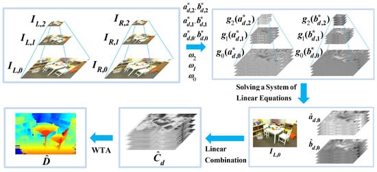
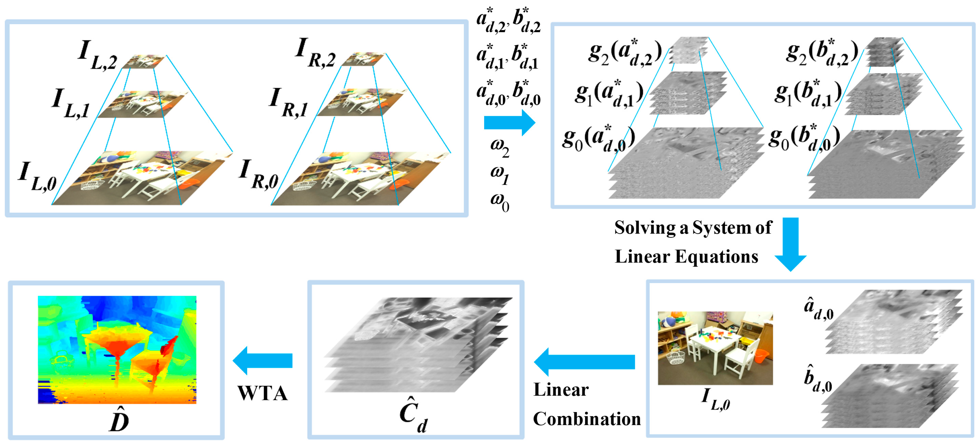
The procedure of our proposed algorithm for stereo matching is depicted in Figure 1, taking K = 2 as an example, and summarized in the following steps:

1. Down-sample the image pairs to build a pair of pyramids of images, $I_{L,z}$ and $I_{R,z}$ for $z\in \{0,1,\dots ,K\}$, with K + 1 levels of resolution;

2. Calculate the weight matrix ${\omega }_z(p,q)$ as a multiplication of two weighting factors, ${\overline{W}}_{i,x,z}^H$ and ${\overline{W}}_{j,y,z}^V$ for $z\in \{0,1,\dots ,K\}$:

$${\omega }_z(p,q)={\overline{W}}_{i,x,z}^H\cdot {\overline{W}}_{j,y,z}^V$$

(19)

where the weighting factors are recursively calculated for $z\in \{0,1,\dots ,K\}$ as:

$$\begin{array}{l}{\overline{W}}_{i,x,z}^H=\{\begin{array}{ll}{\displaystyle \prod _{u=\min (i,x)+1}^{\max (i,x)}\exp \left(\frac{f(|I_{L,z}(u,j)-I_{L,z}(u-1,j)|)}{-\beta }\right),}& i\ne x\\ 1,& i=x\end{array}\\ {\overline{W}}_{j,y,z}^V=\{\begin{array}{ll}{\displaystyle \prod _{u=\min (j,y)+1}^{\max (j,y)}\exp \left(\frac{f(|I_{L,z}(x,u)-I_{L,z}(x,u-1)|)}{-\beta }\right),}& j\ne y\\ 1,& j=y\end{array}\\ \mathrm{with}f(\xi )=\{\begin{array}{ll}0,& \mathrm{if}\xi =0\\ 1,& \mathrm{if}\xi >0\end{array}\end{array}$$

(20)

3. Generate the primary matching cost volume for each scale where $z\in \{0,1,\dots ,K\}$:

$$C_{d,z}(q)=\min (|{\nabla }_x{I}_{L,z}(q)-{\nabla }_x{I}_{R,z}(q+d)|,\tau )+\min (|{\nabla }_y{I}_{L,z}(q)-{\nabla }_y{I}_{R,z}(q+d)|,\tau ).$$

(21)

4. Find the optimum parameters for each resolution, where $z\in \{0,1,\dots ,K\}$:

$$\begin{array}{l}{a}_{d,z}^{*}(p)=\frac{\frac{{\displaystyle \sum _{q\in I_{L,z}(p)}[{\omega }_z(p,q)\cdot I_{L,z}(q)\cdot C_{d,z}(q)]}}{{\displaystyle \sum _{q\in I_{L,z}(p)}{\omega }_z(p,q)}}-\frac{{\displaystyle \sum _{q\in I_{L,z}(p)}[{\omega }_z(p,q)\cdot I_{L,z}(q)]}}{{\displaystyle \sum _{q\in I_{L,z}(p)}{\omega }_z(p,q)}}\cdot \frac{{\displaystyle \sum _{q\in I_{L,z}(p)}[{\omega }_z(p,q)\cdot C_{d,z}(q)]}}{{\displaystyle \sum _{q\in I_{L,z}(p)}{\omega }_z(p,q)}}}{\frac{{\displaystyle \sum _{q\in I_{L,z}(p)}[{\omega }_z(p,q)\cdot I_{L,z}(q)\cdot I_{L,z}(q)]}}{{\displaystyle \sum _{q\in I_{L,z}(p)}{\omega }_z(p,q)}}-{\left\{\frac{{\displaystyle \sum _{q\in I_{L,z}(p)}[{\omega }_z(p,q)\cdot I_{L,z}(q)]}}{{\displaystyle \sum _{q\in I_{L,z}(p)}{\omega }_z(p,q)}}\right\}}^2+\epsilon (p)}\\ b_{d,z}^{*}(p)=\frac{{\displaystyle \sum _{q\in I_{L,z}(p)}[{\omega }_z(p,q)\cdot C_{d,z}(q)]}}{{\displaystyle \sum _{q\in I_{L,z}(p)}{\omega }_z(p,q)}}-a_{d,z}^{*}(p)\cdot \frac{{\displaystyle \sum _{q\in I_{L,z}(p)}[{\omega }_z(p,q)\cdot I_{L,z}(q)]}}{{\displaystyle \sum _{q\in I_{L,z}(p)}{\omega }_z(p,q)}}.\end{array}$$

(22)

5. Calculate the nominal average function to the parameters, $g_z(a_{d,z}^{*}(p))$ and $g_z(b_{d,z}^{*}(p))$, according to Equation (13) for $z\in \{0,1,\dots ,K\}$;

6. Solve for ${\widehat{a}}_{d,0}(p)$ and ${\widehat{b}}_{d,0}(p)$ based on the system of linear Equations (11) and (12);

7. Aggregate the cost volume across multiple scales according to Equation (17);

8. Find the disparity map using the WTA procedure of Equation (18).

As depicted in Figure 1, the parameters ${\widehat{a}}_{d,0}(p)$ and ${\widehat{b}}_{d,0}(p)$ are found by solving the system of linear equations, composed of Equations (11) and (12). As the matrix inverse can be conducted in advance, the calculation can be simplified into matrix multiplication, as demonstrated in Equation (14).

Besides, the cost volume ${\widehat{C}}_d(p)$ is calculated using the linear model of Equation (17). In contrary to the current multi-scale approaches in the literature, such as References [27,28,29], where the cross-scale aggregation is based on costs themselves, the parameter-based cross-resolution aggregation of the proposed procedure is unique and efficient.

3. Experimental Results

In the proposed scheme, there are two design parameters, $\beta$ in Equation (20) and $\gamma$ in Equation (9). According to Equations (19) and (20), we have that larger $\beta$ will cause ${\overline{W}}_{i,x,z}^H$ and ${\overline{W}}_{j,y,z}^V$ to increase, so ${\omega }_z$ is larger and $\widehat{D}(p)$ will be smoother. Based on Equation (9), we also have that when $\gamma$ is larger, the constraint between the scale layers is stronger.

We conducted experiments using the training dataset of the KITTI Vision Benchmark Suite [30] to determine the proper values for these two parameters. The dataset contains 200 image pairs and 200 ground truth disparity maps. The results of the performance of the proposed scheme using the dataset are summarized in Figure 2.

Figure 2a,b display the mean values of the percentage of the erroneous pixels on the disparity maps, denoted as the average error rates, and the standard deviations. Each of the mean values along with the standard deviation was calculated using these 200 image pairs. When $\beta =2$ and $\gamma =1.5$ these two parameters achieved their best performance. We fixed these values for all the calculation experiments presented in this section.

To validate the effectiveness of the proposed scheme, extensive comparative experiments were conducted. We studied six state-of-the-art stereo matching algorithms to compare with the proposed scheme:

• The fast cost volume filtering scheme of Reference [19], denoted as FCVF;
• A combination of the cross-scale cost aggregation scheme of Reference [29] and FCVF [19], denoted as CS-FCVF;
• The pervasive guided-image-filter scheme of Reference [25], denoted as PGIF;
• A combination of the cross-scale cost aggregation scheme of Reference [29] and PGIF [25], denoted as CS-PGIF;
• The deep self-guided cost aggregation scheme of Reference [8], denoted as DSG;
• The sparse representation over discriminative dictionary scheme of Reference [13], denoted as SRDD;
• The proposed scheme, which implements a hierarchical guided-image-filter, denoted as HGIF.

We tested these frameworks using the Middlebury (version 3) benchmark stereo database downloaded via the URL: vision.Middlebury.edu/stereo/ [31]. The “trainingQ” image set, which contains 15 stereo pairs, were used for the performance evaluation, starting from “Adirondack” to “Vintage”. Of them, only five are shown in Figure 3 due to the space limitation. They are: “Adirondack”, “Pipes”, “Playroom”, “Playtable”, and “Shelves”. These pictures are with a typical resolution of 720 by 480. These image pairs are down-sized twice, to 360 by 240 and 180 by 120, for example, in the proposed scheme. This arrangement corresponds to K = 2.

Besides, the Middlebury defines two measures for evaluating average error rates, including non-occluded (non-occ) and all regions. The weighted average error rate is an official metric of the benchmark in measuring the accuracy of matching by using different weights for different image pairs. These weights are employed to compensate for the variation in the matching difficulty, as remarked on the website. Specifically, the image pairs: “PianoL”, “Playroom”, “Playtable”, “Shelves”, and “Vintage” contribute only half of the error rates.

Figure 4 shows the disparity maps obtained by these algorithms. Among them, only the results of SRDD [13] were improved by the disparity refinement procedure. The corresponding error rates in the non-occluded region and the all-region are summarized in

Table 1. Comparison of the weighted average error rates in the non-occluded (non-occ) region between seven algorithms (%). All of the results are obtained without the refinement procedure except SRDD [13]. The lowest error records are marked in bold.

Image Sets	FCVF	CS-FCVF	PGIF	CS-PGIF	DSG	SRDD	Proposed
Adirondack	8.78	7.93	6.43	6.30	8.98	6.53	5.73
ArtL	12.22	12.20	10.90	10.78	13.79	13.17	10.85
Jadeplant	21.81	22.85	20.03	20.43	21.22	18.98	19.67
Motorcycle	9.87	9.58	9.01	8.88	8.66	9.02	8.45
MotorcycleE	9.72	9.27	8.93	8.60	7.78	7.69	8.47
Piano	16.20	14.65	14.01	13.53	17.55	14.88	14.02
PianoL	33.44	33.10	30.25	30.61	31.41	26.65	29.32
Pipes	10.45	10.87	9.96	10.49	12.38	11.67	9.85
Playroom	22.68	19.41	16.62	15.63	23.98	16.25	15.18
Playtable	41.89	20.04	39.29	20.77	36.67	18.34	16.71
PlaytableP	13.81	12.10	13.08	11.25	19.91	10.55	10.98
Recycle	10.52	10.75	8.38	9.16	11.44	9.18	8.28
Shelves	39.52	34.52	36.11	31.92	41.13	37.88	31.63
Teddy	7.18	6.60	6.33	5.27	8.24	6.26	5.57
Vintage	33.22	29.73	30.05	29.83	33.53	27.30	26.97
Weighted Average	16.47	14.82	14.66	13.53	17.06	13.69	12.94

and

Table 2. Comparison of the weighted average error rates in the all-region between seven algorithms (%). All of the results are obtained without the refinement procedure except SRDD [13]. The lowest error records are marked in bold.

Image Sets	FCVF	CS-FCVF	PGIF	CS-PGIF	DSG	SRDD	Proposed
Adirondack	10.09	9.64	8.39	8.82	15.58	8.77	7.96
ArtL	21.90	22.02	21.64	21.23	30.79	22.86	21.17
Jadeplant	34.51	35.87	33.45	33.89	38.02	32.47	33.00
Motorcycle	13.50	13.34	13.23	13.18	17.52	13.54	12.62
MotorcycleE	13.68	13.13	13.25	13.17	16.68	11.96	12.92
Piano	19.99	18.61	18.29	17.74	23.48	19.30	18.11
PianoL	36.43	36.14	33.91	34.13	36.15	30.49	33.09
Pipes	21.45	22.01	21.52	22.10	26.28	22.88	21.49
Playroom	30.61	27.88	25.38	24.32	33.93	25.11	23.79
Playtable	44.65	24.39	42.63	25.57	42.70	23.29	21.23
PlaytableP	17.29	15.00	17.55	15.43	27.74	14.39	14.28
Recycle	12.30	12.58	10.50	11.59	17.50	11.51	10.33
Shelves	40.14	35.43	36.89	32.91	44.43	39.15	32.64
Teddy	12.59	12.14	11.94	10.96	17.48	11.75	11.19
Vintage	37.18	33.86	34.01	33.67	38.47	31.51	30.94
Weighted Average	21.74	20.26	20.49	19.47	26.31	19.54	18.71

, respectively.

Taking a close look of the disparity maps of Figure 4, we have that there was a significant improvement in the matching quality of CS-FCVF [19,29] over FCVF [19], especially in the texture-less regions of the “Playtable” and “Shelves” cases. This improvement was less significant but could also be observed in that of the CS-PGIF [25,29] over PGIF [25]. These improvements were due to the effective cross-scale cost aggregation scheme of Reference [29].

According to the weighted average error rates listed in Table 1 and Table 2, DSG [8] performed worst. Also, the matching performance of SRDD [13] was better than CS-FCVF [19,29] but slightly worse than CS-PGIF [25,29]. It is worthy to note that SRDD [13] applies semi-global cost aggregation and post-processing refinement to further improve the matching accuracy. However, the proposed scheme, even without refinement, performed better than SRDD [13] in most of the cases and achieves the smallest weighted average error rates in both the all-region and the non-occluded (non-occ) region.

The experiment was executed in MATLAB 2017b using an Intel Core I5 8300H and 16 GB RAM.

Table 3. Comparison of the computation time for four selected image sets between five algorithms (s).

Methods	Adirondack	Playroom	Playtable	Shelves
FCVF	15	16	14	15
CS-FCVF	20	21	18	18
PGIF	23	24	22	22
CS-PGIF	28	29	26	26
Proposed	31	31	29	29

summarizes the execution time of these algorithms. We have that the multi-scale versions, CS-FCVF [19,29] and CS-PGIF [25,29], required more time for computation than their original versions, FCVF [19] and PGIF [25], respectively, as expected.

Similarly, the proposed algorithm needed to calculate the filtering parameters in multiple scale layers, it ran longer than the FCVF algorithm [19] and the PGIF algorithm [25]. In addition, the CS-FCVF [19,29] and CS-PGIF [25,29] algorithms only incorporated one matching cost parameter, while the proposed algorithm has to compute two parameters, ${\widehat{a}}_{d,0}(p)$ and ${\widehat{b}}_{d,0}(p)$ in Equations (11) and (12). We also have that the proposed algorithm ran slightly longer than CS-FCVF [19,29] and CS-PGIF [25,29]. However, the increased computation time was marginal and still within the same order of magnitude. Moreover, both DSG [8] and SRDD [13] required much more computational resource than the other algorithms due to their deep neural network and semi-global cost aggregation scheme, respectively, as pointed out in Reference [13]. Based on Table 3, we may conclude that the proposed scheme had the best performance when taking both the matching correctness and the calculation efficiency into consideration.

4. Conclusions

In this work, we propose a novel stereo matching scheme to make use of hierarchical pattern information in stereo matching. The scheme exploits feature with different level of scales for matching metrics.

Inspired by the scheme of Zhang [29] for multi-scale disparity cost aggregation, the scheme uses a hierarchy of parameters of the GIF-based linear models and exploits the pervasive guided-image-filtering [25] for efficient matching cost calculation. The resultant multi-scale features are collected to form an improved cost volume for disparity estimation by using a linear combination of the guidance image.

A performance evaluation of version 3 of the Middlebury stereo evaluation data set [31] showed that the proposed solution provided superior disparity accuracy and comparable processing speed when compared with the representative stereo matching algorithms. Besides, the scheme outperformed most of the state-of-art algorithms even without the refinement procedure.

References

- Scharstein, D.; Szeliski, R. A taxonomy and evaluation of dense two-frame stereo correspondence algorithms. Int. J. Comput. Vis. 2002, 47, 7–42. [Google Scholar] [CrossRef]
- Zbontar, J.; LeCun, Y. Stereo matching by training a convolutional neural network to compare image patches. J. Mach. Learn. Res. 2016, 17, 1–32. [Google Scholar]
- Nahar, S.; Joshi, M.V. A learned sparseness and IGMRF-based regularization framework for dense disparity estimation using unsupervised feature learning. IPSJ Trans. Comput. Vis. Appl. 2017, 9, 1–15. [Google Scholar] [CrossRef]
- Mayer, N.; Ilg, E.; Hausser, P.; Fischer, P.; Cremers, D.; Dosovitskiy, A.; Brox, T. A large dataset to train convolutional networks for disparity, optical flow, and scene flow estimation. In Proceedings of the IEEE Conference on Computer Vision and Pattern Recognition, Las Vegas, NV, USA, 27–30 June 2016; pp. 4040–4048. [Google Scholar]
- Pang, J.; Sun, W.; Ren, J.S.; Yang, C.; Yan, Q. Cascade residual learning: A two-stage convolutional neural network for stereo matching. In Proceedings of the IEEE International Conference on Computer Vision Workshops, Venice, Italy, 22–29 October 2017; pp. 878–886. [Google Scholar]
- Kendall, A.; Martirosyan, H.; Dasgupta, S.; Henry, P.; Kennedy, R.; Bachrach, A.; Bry, A. End-to-end learning of geometry and context for deep stereo regression. In Proceedings of the IEEE International Conference on Computer Vision, Venice, Italy, 22–29 October 2017; pp. 66–75. [Google Scholar]
- Chang, J.R.; Chen, Y.S. Pyramid stereo matching network. In Proceedings of the IEEE Conference on Computer Vision and Pattern Recognition, Salt Lake City, UT, USA, 18–22 June 2018; pp. 5410–5418. [Google Scholar]
- Park, I.K. Deep self-guided cost aggregation for stereo matching. Pattern Recognit. Lett. 2018, 112, 168–175. [Google Scholar]
- Pan, C.; Liu, Y.; Huang, D. Novel belief propagation algorithm for stereo matching with a robust cost computation. IEEE Access 2019, 7, 29699–29708. [Google Scholar] [CrossRef]
- Yao, P.; Zhang, H.; Xue, Y.; Chen, S. As-global-as-possible stereo matching with adaptive smoothness prior. IET Image Process. 2019, 13, 98–107. [Google Scholar] [CrossRef]
- Gupta, R.K.; Cho, S.Y. Stereo correspondence using efficient hierarchical belief propagation. Neural Comput. Appl. 2012, 21, 1585–1592. [Google Scholar] [CrossRef]
- Hu, T.; Qi, B.; Wu, T.; Xu, X.; He, H. Stereo matching using weighted dynamic programming on a single-direction four-connected tree. Comput. Vis. Image Underst. 2012, 116, 908–921. [Google Scholar] [CrossRef]
- Yin, J.; Zhu, H.; Yuan, D.; Xue, T. Sparse representation over discriminative dictionary for stereo matching. Pattern Recognit. 2017, 71, 278–289. [Google Scholar] [CrossRef]
- Yoon, K.J.; Kweon, I.S. Adaptive support-weight approach for correspondence search. IEEE Trans. Pattern Anal. Mach. Intell. 2006, 28, 650–656. [Google Scholar] [CrossRef] [PubMed]
- Yang, Q. Stereo matching using tree filtering. IEEE Trans. Pattern Anal. Mach. Intell. 2015, 37, 834–846. [Google Scholar] [CrossRef]
- Pham, C.C.; Jeon, J.W. Domain transformation-based efficient cost aggregation for local stereo matching. IEEE Trans. Circuits Syst. Video Technol. 2013, 23, 1119–1130. [Google Scholar] [CrossRef]
- Çığla, C.; Alatan, A.A. An efficient recursive edge-aware filter. Signal Process. Image Commun. 2014, 29, 998–1014. [Google Scholar] [CrossRef]
- Yang, Q.; Li, D.; Wang, L.; Zhang, M. Full-image guided filtering for fast stereo matching. IEEE Signal Process. Lett. 2013, 20, 237–240. [Google Scholar] [CrossRef]
- Hosni, A.; Rhemann, C.; Bleyer, M.; Rother, C.; Gelautz, M. Fast cost-volume filtering for visual correspondence and beyond. IEEE Trans. Pattern Anal. Mach. Intell. 2013, 35, 504–511. [Google Scholar] [CrossRef]
- He, K.; Sun, J.; Tang, X. Guided image filtering. IEEE Trans. Pattern Anal. Mach. Intell. 2013, 35, 1397–1409. [Google Scholar] [CrossRef] [PubMed]
- Li, Z.; Zheng, J.; Zhu, Z.; Yao, W.; Wu, S. Weighted guided image filtering. IEEE Trans. Image Process. 2014, 24, 120–129. [Google Scholar]
- Kou, F.; Chen, W.; Wen, C.; Li, Z. Gradient domain guided image filtering. IEEE Trans. Image Process. 2015, 24, 4528–4539. [Google Scholar] [CrossRef] [PubMed]
- Hong, G.S.; Kim, B.G. A local stereo matching algorithm based on weighted guided-Image-filtering for improving the generation of depth range images. Displays 2017, 49, 80–87. [Google Scholar] [CrossRef]
- Zhu, S.; Yan, L. Local stereo matching algorithm with efficient matching cost and adaptive guided image filter. Vis. Comput. 2017, 33, 1087–1102. [Google Scholar] [CrossRef]
- Zhu, C.; Chang, Y.Z. Efficient stereo matching based on pervasive guided image filtering. Math. Probl. Eng. 2019, 2019, 1–11. [Google Scholar] [CrossRef]
- Hu, W.; Zhang, K.; Sun, L.; Yang, S. Comparisons reducing for local stereo matching using hierarchical structure. In Proceedings of the IEEE International Conference on Multimedia and Expo, San Jose, CA, USA, 15–19 July 2013; pp. 1–6. [Google Scholar]
- Tang, L.; Garvin, M.K.; Lee, K.; Alward, W.L.M.; Kwon, Y.H.; Abràmoff, M.D. Robust multiscale stereo matching from fundus images with radiometric differences. IEEE Trans. Pattern Anal. Mach. Intell. 2011, 33, 2245–2258. [Google Scholar] [CrossRef] [PubMed]
- Li, R.; Ham, B.; Oh, C.; Sohn, K. Disparity search range estimation based on dense stereo matching. In Proceedings of the IEEE Conference on Industrial Electronics and Applications, Melbourne, Australia, 19–21 June 2013; pp. 753–759. [Google Scholar]
- Zhang, K.; Fang, Y.; Min, D.; Sun, L.; Yang, S.; Yan, S.; Tian, Q. Cross-scale cost aggregation for stereo matching. In Proceedings of the IEEE Conference on Computer Vision and Pattern Recognition, Columbus, OH, USA, 23–28 June 2014; pp. 1590–1597. [Google Scholar]
- Moritz, M.; Geiger, A. Object Scene Flow for Autonomous Vehicles. In Proceedings of the Conference on Computer Vision and Pattern Recognition (CVPR), Boston, MA, USA, 8–10 June 2015; pp. 1–10. [Google Scholar]
- Scharstein, D.; Hirschmüller, H.; Kitajima, Y.; Krathwohl, G.; Nesic, N.; Wang, X.; Westling, P. High-resolution stereo datasets with subpixel-accurate ground truth. In Proceedings of the German Conference on Pattern Recognition (GCPR 2014), Münster, Germany, 12–15 September 2014; pp. 1–12. [Google Scholar]
Figure 1.
An overview of the proposed stereo matching process with two levels of down-sampling as an example.
Figure 2.
The effect of parameter selection on the performance of the proposed scheme using 200 stereo image pairs of the training dataset in the KITTI Vision Benchmark Suite [30]. The dataset was downloaded from the URL: www.cvlibs.net/datasets/kitti/index.php. Each figure shows the mean values of the error rates and their corresponding standard deviations. (a) The average error rate with respect to the parameter when = 1.5. (b) The average error rate with respect to the parameter when = 2.
Figure 3.
Datasets and their corresponding ground truth disparity maps selected from the experimented data for visual comparison. (a) Left images of the image pairs: Adirondack, Pipes, Playroom, Playtable, and Shelves; (b) ground truth disparity maps of these images. Image courtesy of the Middlebury (version 3) benchmark stereo database via the URL: vision.middlebury.edu/stereo/ [31].
Figure 4.
Comparisons of disparity maps obtained by different algorithms. All the results are obtained without the refinement procedure except SRDD (The sparse representation over discriminative dictionary scheme) [13]. (a–g) are disparity maps generated by: (a) FCVF (The fast cost volume filtering scheme) [19], (b) CS-FCVF (A combination of the cross-scale cost aggregation scheme [29] and FCVF), (c) PGIF (The pervasive guided image filter scheme) [25], (d) CS-PGIF (A combination of [29] and PGIF), (e) DSG (The deep self-guided cost aggregation scheme) [8], (f) SRDD (The sparse representation over discriminative dictionary scheme) [13], and (g) the proposed scheme. Among them, the images of (e) DSG and (f) SRDD are by courtesy of the Middlebury (version 3) benchmark stereo database via the URL: vision.middlebury.edu/stereo/ [31].