Abstract
Non-intrusive load monitoring (NILM) is a core technology for demand response (DR) and energy conservation services. Traditional NILM methods are rarely combined with practical applications, and most studies aim to disaggregate the whole loads in a household, which leads to low identification accuracy. In this method, the event detection method is used to obtain the switching event sets of all loads, and the power consumption curves of independent unknown electrical appliances in a period are disaggregated by utilizing comprehensive features. A linear discriminant classifier group based on multi-feature global similarity is used for load identification. The uniqueness of our algorithm is that it designs an event detector based on steady-state segmentation and a linear discriminant classifier group based on multi-feature global similarity. The simulation is carried out on an open source data set. The results demonstrate the effectiveness and high accuracy of the multi-feature integrated classification (MFIC) algorithm by using the state-of-the-art NILM methods as benchmarks.
1. Introduction
Increased public awareness of energy conservation in recent years motivates electricity consumers to participate in energy management actively [1]. Demand response (DR) is one of the solutions for demand side management, which responds to certain conditions by reducing or shifting loads to a different time period. With the advent of the smart grid, residential DR has great research potential. Since different types of appliances have different opportunities and ways to participate in DR, it is crucial to study detailed appliance-level power consumption. In addition, the visualization of detailed consumption of high-power appliances will help customers to replace some inefficient devices, so as to save energy [2].
Traditional intrusive load monitoring needs to install lots of sensors to acquire a signal of each appliance. In the process of sensors’ installation and maintenance, the power supply needs to be temporarily interrupted, which causes inconvenience for both the power grid and users. Due to the poor practicability of the intrusive method, Hart proposed the concept of non-intrusive load monitoring (NILM) in the 1980s [3]. Since it has a lower installation cost and impact for users, NILM is more attractive to customers and utilities. The main idea of NILM is disaggregating mixed electrical signals acquired at power entrance to obtain the working status and detailed power consumption information of individual appliances.
Early studies in NILM focused on detecting state-changing events by identifying distinct electrical features of individual appliances, which are called “load signature” and can be divided into two categories: steady-state and transient state. It is a good idea to complete NILM with unsupervised learning by combining different features [4]. The most commonly used steady-state signatures are active and reactive power [2,5]. They are effective in identifying high-power devices, but it is challenging to separate low-power appliances for them due to the possibility of power overlap. Later works extended the steady-state signature to many aspects, such as harmonics [6], current and voltage waveforms [7], voltage-current trajectory [8,9,10], inactive current [11] etc. All of them can disaggregate certain types of appliances effectively. In order to define more accurate load signatures, features are extracted from the period of two stable operations, called transient signature [12,13,14]. Due to a relatively shorter duration of transient signatures, the probability of feature overlapping is lower. Transient signatures require a high sampling rate. However, it is difficult to achieve high sampling rate in practical applications, which limits the practicability of transient signatures.
With the large-scale deployment of smart meters, NILM approaches that work with a lower sampling rate have drawn increasing attention. Most smart meters installed in practical applications measure and transmit the power signals at a relatively low frequency, generally between 1 Hz and 1/900 Hz [15]. Consequently, the steady-state signatures become a more suitable choice in applications. Low-rate NILM methods can be divided into two categories. One refers to event-based NILM [16], which implements load monitoring by classifying the signatures related to load events. The other is state-based NILM [17], which realizes load disaggregation through pattern recognition.
Most of state-based NILM methods are based on the hidden Markov model (HMM) and its variations [18,19,20,21] due to the strong ability in modeling the combination of stationary process with continuous valued data over discrete time. Yuan proposes a load disaggregation method based on clustering algorithm and support vector regression optimization, which works very well [22]. Four different extensions of HMM are presented [20], but they are likely to converge to a local minimum. To address this problem, the hierarchical Dirichlet process hidden semi-Markov mode (HDP-HSMM) is described [21]. To extend NILM service to new households without further intrusive monitoring, a model fitting algorithm is designed [23], which adopts iterative k-means to fit a HMM with only one typical duty cycle of device. However, HMM has heavy dependence on clean transitions from one state to another, especially for continuously varying appliances. To alleviate this problem, a sparse coding method based on structured prediction is developed [24]. Motivated by the success of deep learning, a deep sparse coding is proposed [25]. However, a typical shortcoming is that more parameters need to be learned for going deeper. Kelly uses a neural network to complete the load disaggregation problem and gets good results [26]. But generally, state-based algorithms have a common drawback, i.e., long periods of training and high computational complexity, which makes them difficult to apply to real-time disaggregation.
Event-based algorithms have a relatively fixed processing procedure, including event detection, feature extraction and event classification. To obtain accurate identification results, different classification techniques are tried, including k-means [27], k-nearest neighbor (k-NN) [28], naïve Bayes [29], maximum likelihood [30] and decision tree (DT) [31]. In [30] the maximum likelihood classifier is designed to disaggregate load based on the power profiles, but it only works for single-state loads. Zhao relies on graph signal processing (GSP) to realize the edge detection, clustering, and pattern matching [31]. However, experimental results show that power fluctuation or a close power range of appliances will influence algorithm performance. Qi adopts graph shift quadratic form constraint to complete low-rate load disaggregation [32]. A novel combined k-means-SVM-based NILM method is developed [33]. However, event-based methods face a common challenge, that is, most of the existing algorithms only rely on a two-dimensional feature space of active and reactive power for load identification without considering other additional features, such as time and sequence signatures. Moreover, the same type of appliances in different households have quite different signatures, so it is unsuitable to use a unified model to represent them.
The existing NILM methods are focused on detection of all appliances without considering the applicability of load disaggregation in realistic applications, that is, there is no definition of an accurate load space related to the actual application. Load space refers to the range of load types to be analyzed. In this paper, we define different load types that need to be analyzed. It also describes which loads belong to different types. Because of the complexity of the original load space, it is impractical to identify all devices based on a one-dimensional aggregated signal. So, there is an emerging need to define a suitable load space.
In order to address the difficulty of identifying appliances with similar power, a linear discriminant classifier group considering multidimensional features is designed in this paper. It is an event-based method, which can work seamlessly with smart meter infrastructure without installing additional acquisition devices. Considering the practical application of this study is to provide appliance-level information for DR and energy-saving service, the types of the monitored load can be narrowed down to some controllable and high-power loads.
This work formalizes a load identification technique based on the multi-feature integrated classification (MFIC), where the only input is the time-stamped power readings from the smart meter. The major contributions of this paper are as follows:
- (1)
- Considering the different operating habits and inherent electrical characteristics of loads, multidimensional features are used to model each appliance and improve the load discrimination. In addition, due to the great difference of appliances signatures in different households, this paper uses proprietary model database to replace the uniform feature database.
- (2)
- Based on steady-state segmentation, a designed event detector in this paper has fewer parameters and no dependence with the detection window.
- (3)
- A linear discriminant classifier for each appliance is designed according to the overall similarity of multi-features. Based on the designed discriminant classifiers, a discriminant classifier group can be formed.
The structure of this paper is given as follows. Section 2 selects multidimensional features for load modeling. In addition, a brief analysis of DR and energy-saving services is made to specify the research objective and narrow down the load space. Section 3 elaborates on the problem definition and the complete process of proposed MFIC algorithm. Section 4 presents experiments and their results. The last section concludes the paper and discusses future works.
2. Appliance Modeling
2.1. Appliance Behaviour Modelling
The aim of NILM is to identify the electrical appliances inside the user. The schematic diagram is shown in Figure 1. Self-adaptive establishment of an exclusive appliance model library for different users is important to non-intrusive load identification. The NILM acquires the comprehensive power consumption data at the power supply entrance. The power consumption data of all loads is included in one collected signal, out of which the power consumption information of individual loads should be separated and extracted. Therefore, exploiting distinguishable features to model appliance behavior is a significant work for NILM.
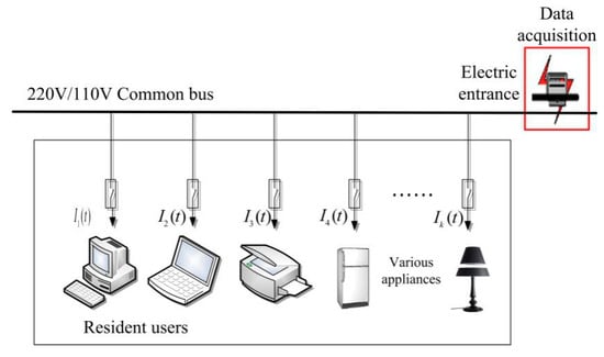
Figure 1.
The schematic diagram of non-intrusive load monitoring (NILM).
Low-frequency signals contain less load information, so most of the existing low-rate NILM studies can only use power indicators to characterize devices. The power values of some electrical appliances are very close, so the accuracy is low when power is the only feature of identification. In fact, the operating features of the load can be extracted from the load data. Through the analysis of the concrete operation process of each appliance, some distinguishing features can be found. The power consumption curves of several typical appliances are shown in Figure 2.
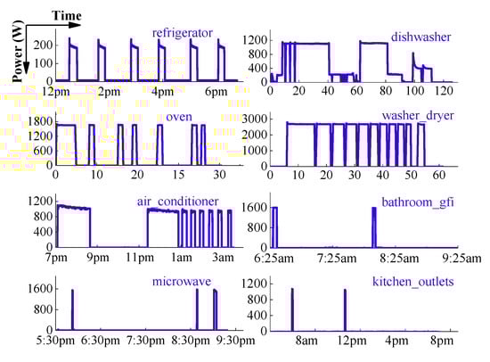
Figure 2.
Load profiles of eight typical appliances.
Figure 2 presents power consumption curves of several typical appliances, which show regular operating features. As presenting a fixed working cycle and interval time in Figure 2, the refrigerator runs in a periodic cycle for 15 min and closes for 51 min. A complete operation cycle of the dishwasher can be divided into three main stages: wash, rinse and dry. The operation cycle is determined by its internal structure. An oven is also an intermittent running load, but the ON/OFF-duration is not fixed. The operation time is between 15 min and 1 h, decided by the users’ setting. Observing the curve of washer dryer, we can find that the longest time is the first ON time followed by several ON/OFF cycles. The number of ON/OFF cycles is related to laundry loads.
In this work, the following eight features are selected, divided into two categories, i.e., intrinsic features and statistical features. Intrinsic features, known as the electrical features, are determined by the appliance itself. Statistical features reflect users’ habits of using specific appliances, which can be called non-electrical features [34]. For example, TV is used more in the evening than daytime, and the lamp has similar statistical features.
Intrinsic features include the following four criteria:
- Active power change. This refers to the event caused by the state transition of appliances, and appears as the rising or falling edge. The typical appliances can be divided into three types: single-state, continuous varying and multi-state. The single-state load has a pair of identical rising/falling edges and constant power consumption between them, such as microwave. A continuous varying load such as refrigerator generally has a pair of different rising/falling edges and the power consumption during operation is continuously changing. Multi-state load has more than one working stage, such as a dishwasher.
- On-duration. This refers to the continuous operating time in a periodic cycle, which is mainly applied to the loads with fixed operating periods, such as a refrigerator. As mentioned above, the On-duration of the refrigerator is 15 min.
- Off-duration. It stands for the continuous standby time in a periodic cycle. For instance, the Off-duration of refrigerator is 51 min. Figure 3 illustrates the On-duration and Off-duration of refrigerator in a cycle.
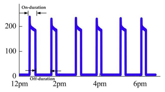 Figure 3. The On-duration and Off-duration of refrigerator in a cycle.
 - On times. This means the number of turning on contained in each operation cycle. The “On times” is used for identification of household appliances with a fixed operating process, such as dishwashers. The dishwasher experiences the same process every time in a complete washing process. Observing the power consumption curve during the whole washing process, we can find that the times of high power operation mode fluctuate near a stable value, and so do the low power operation mode. Since this fully automatic dishwasher has a fixed operation washing process, the “On times” remains unchanged.
Statistical features serve to emphasize the users’ habits of using specific appliances, including the following four kinds:
- Switching-time. This refers to the possible switching on/off time, which is related to the function of an appliance.
- Usage frequency in one day. This refers to the times that the load may be opened in a day. There are many appliances operating in an ON/OFF cycle, such as an oven, air conditioner and washer dryer. When calculating the usage frequency of loads in a day, it is necessary to ensure that a complete operation process is counted once.
- Working days in a week. This means the days that an appliance may work within a week. For example, a refrigerator is a constant-opening device, while washing machine is less likely to be used every day.
- Duration of a complete use process. This is used to record the duration of an appliance from start to shut down, including all subsequences ON/OFF cycles.
2.2. Determine the Load Space to be Monitored
As described in the introduction, it is difficult to identify all appliances by using a single identification approach, so it is essential to build a reasonable load space according to the specific application of NILM.
Load is classified into three categories according to the state of participating demand response (DR): uncontrollable load (UCL), transferable load (TL) and interruptible load (IL). UCL refers to the load that has no energy storage capacity and may be opened at any time. It has no capacity to transport power consumption basically and its fluctuation range is small. TL is a type of load that can transport the energy consumption, because the using time is flexible and the power consumption is fixed, such as washing machine and electric rice cooker. Consequently, on the premise of the completion of the work requirements, it can participate in DR by changing the running time. An air conditioner and water heater are typical ILs, which can be interrupted temporarily without affecting consumer comfort to reduce the power consumption. On the contrary, the interruption of UCL is likely to affect consumer’s comfort, so TL and IL will be treated in different ways in DR, and managed centrally at the control center after the load identification. It is necessary to divide TL and IL into different load spaces in identification.
The adjustable high-power loads are suitable for participating in DR, so the research mainly focuses on identifying the adjustable high-power loads, while there is no need to track the appliances with small power. The final load space to be monitored is listed in Table 1. In addition, because there are too many UCLs in a family, such as a TV and computer, we use high-power electrical appliances to refer to a large number of loads in Table 1. This does not mean that the number or proportion of UCLs in user families is small. We classify all electrical appliances in the family to achieve the goal of mainly studying IL and TL.

Table 1.
Load space to be monitored.
3. Methodology
3.1. Load Disaggregation Definition
The definition of load disaggregation can be expressed as follows: Given the mixed signal collected at the power entrance of a house, we need to disaggregate the mixed signal into a series of individual components attributed to specific appliances. The mixed signal consists of individual appliance signals which are switched ON at the given moment. It is necessary to design a Boolean coefficient an,m(k), which determines whether the mode m of appliance n is ON at the kth sampling point. Mathematically, the mixed signal obtained can be formulated as a linear combination of some unknown appliance power consumption data, which is shown as Equation (1).
where, P(k), k = 1,2,3,…,L is the aggregated power signal (L is the number of samples) and pn,m(k) denotes the individual power consumption of appliance n in mode m. N and M are the number of appliances and modes, respectively. e(k) stands for the noise signal and small appliances whose power is very small so that they have little effect on mixed signals, including phone chargers, DVD player and so on. So it can be ignored in load identification. The objective is to decode P(k) and obtain the status of each appliances by using a set of appliance models in the house.
In existing research, subjected to some prior information, combination optimization is a common method to solve the Equation (1), which searches the optimum appliance status by minimizing the difference between the actual aggregate power and the sum of disaggregated appliance powers.
3.2. Algorithm Overview
In reality, appliances may not operate at their rated power, because the actual power consumption is proportional to the power of total load. Furthermore, different appliances may operate in similar electrical signature “power”. It is difficult to solve the problem in Equation (2) by combination optimization.
The actual electric data display that it is easy to segment the total signal into some steady-state process by clearly step changes. Therefore, an event-based algorithm is designed to solve the load disaggregation problem, including three steps: (1) event detection and clustering, (2) event paring and electrical feature extraction and (3) feature matching. Firstly, we detect the significant active power changes, which represents that some appliances changed their status. Then, events with similar power should be grouped, i.e., clustering. After the formation of clusters, events in “positive” clusters require to be paired with those in negative clusters. Finally, extract the features from each positive-negative cluster pair, and match them with the appliance models. The flowchart is illustrated in Figure 4.
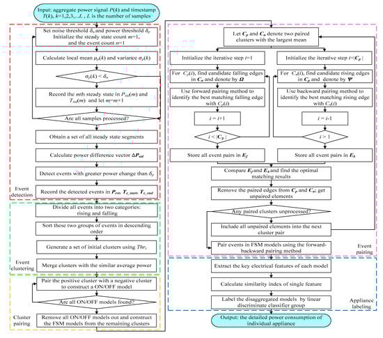
Figure 4.
Flowchart of the proposed algorithm.
3.3. Steady-State Segment Based Event Detection
One important characteristic of event-based load disaggregation is to detect the significant rising or falling edge in active power, and record the power value and occurrence time of events. This paper presents an event detection method based on steady-state segment. It has two parameters, one is noise threshold dn, the other is power threshold dp. The schematic diagram of the event detection is shown in Figure 5.
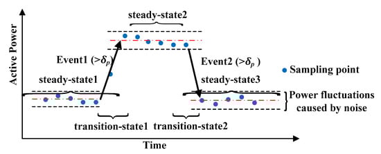
Figure 5.
Schematic diagram of the event detection.
Each appliance can be represented by two states: (1) steady state, including ON and OFF state; and (2) transition state, i.e., the process of changing operation state of multi-state appliance. As long as the steady-state segments are identified, the duration of the power-on or power-off processes for different appliances can be determined adaptively. Load switching is successively based on the switch continuity principle [3], i.e., only one state transition can occur within the sampling time interval. It is feasible to use the step power variation in aggregated signal as the discriminant feature of event occurrence.
The power grid noise exists in the actual electric environment all the time. Low-frequency data can largely avoid noise interference, because the sampling frequency is much less than the noise frequency. In order to further improve the accuracy of the algorithm, the noise threshold is introduced to minimize the possibility of noise impact. Considering the robust to the possible variation of power amplitude caused by the noise, an appropriate event extraction method is designed. The local mean and variance of power are used to capture the load steady state. Assuming P(k), k = 1,2,3,…,L is a given aggregate power signal and T(k), k = 1,2,3,…,L is the corresponding timestamp. By calculating the power changes at a certain time point, as well as before and after two time points, we can judge whether the household appliances are running steadily at that time. Two quantities are be calculated by Equations (3) and (4), where the former is the local mean power and the latter is the local variance.
The reason for choosing 1/3 is that it represents the mean and variance of three time points.
Let δn2 denote the noise variation in power grid. If σp(k) < δn, P(k) is considered in a steady state and then two variables Pstd(m) and Tstd(m) are added to record the mth steady state, shown as follows.
After all the steady state segments are identified, the power difference between two consecutive steady states is calculated as Equation (7):
Set by users, the value of power threshold δp depends on the load events they are interested in. For example, if users focus on the events with power change greater than 100 W, they can set δp = 100. If abs(△Pstd(m))> δp, it indicates that a new event is detected. The power value and timestamp of this event can be obtained as:
where n represents the nth event. Pevt(n) stands for the power value of the nth event, Te_start(n) and Te_end(n) stand for the start time and end time of the event, respectively.
3.4. Event Clustering
The collection of the registered events Pevt(n), n = 1,2,…,Ne is the basis of the event clustering. Ne denotes the number of events detected. Each state of appliances has a unique value and only one appliance may have state transition in one sampling interval, it is reasonable to gather events with similar value into one cluster. Each cluster represents one kind of state transition of appliance.
The proposed clustering algorithm without prior knowledge can adaptively determine the number of clusters. There are two steps:
Step (1): separate the rising and falling edges of the event candidates into two collections of Pevt_up and Pevt_down. Then the rising and falling edges are arranged in descending order according to the absolute value of power, respectively. Set cluster threshold as Thrc. When the difference between two consecutive rising or falling edges is greater than Thrc, a new cluster is generated. The value of Thrc is set small so that the clustering results are more detailed. However, the event caused by the same appliance is also easy to separate some events into different clusters wrongly because of the power fluctuation. In order to solve this problem, we merge some clusters with the similar average power. The detailed process is illustrated in step 2.
Step (2): calculate the mean power of each cluster, and the mean power difference between two adjacent clusters is obtained. If the difference is less than a certain value, it can be considered that these two adjacent clusters belong to the same appliance state. Thus, we will merge them and the new cluster candidates will be formed.
3.5. Building Appliance Candidate Model
After clustering the events, “positive” clusters containing rising edges and “negative” clusters composed of falling edges are obtained. Then, the pairing method is designed to generate appliance candidate models automatically.
Most of the existing NILM algorithms only consider the single-state appliances, so the identification of multi-state loads is limited. The multi-state appliances are very common which cannot be described by ON/OFF model, so it is necessary to establish an appropriate model for them. The finite state machine (FSM) [1] is a typical model for these appliances. The sum of power changes in any cycle of state transition is zero, which can be called zero loop-sum constraint (ZLSC) [1]. Meanwhile, the operating states in an FSM model have different power levels, i.e., uniqueness constraint (UC). The two constraints ensure that it is possible to construct individual FSM from streams of events.
In the following, the method of generating appliance models is introduced. For the single-state appliances, an interruption model is established, and for controllable load, a FSM model is established. It includes two main steps, i.e., cluster pairing and event pairing.
Step (1): to construct ON/OFF models for the single-state appliance candidates, this paper pairs the “positive” cluster and “negative” cluster with similar absolute average power. We take advantage of special algebraic properties of events in a complete transition cycle, i.e., ZLSC and UC, to construct the FSM models. In order to reduce the complexity of cluster pairing, the ON/OFF models are built firstly. After the completion of all positive-negative cluster pairs, they are removed from the total clusters and FSM models are established from the other clusters.
Step (2): after the cluster pairing, some cluster pair candidates for single-state or finite-state appliances will be generated. It is essential to further match the events in each cluster pair. For example, each rising edge in the positive cluster is matched with a falling edge in the paired negative cluster by difference in the pairing features of two events. Then, a specialized forward-backward pairing procedure is designed to realize the effective pairing.
Let Cp and Cn denote two paired clusters, where |Cp| and |Cn| denote their cardinality.
(a) Forward Pairing
For each Cp(i)∈Cp, the forward pairing is to match an optimal falling edge among all elements in Cn according to the order from i = 1 to |Cp|-1. Normally, the ON and OFF events appear alternately, that is, using time stamps to sort events belonging to the same appliance will get an ON/OFF/ON/OFF… sequence. Thus, the falling edge paired with Cp(i) must occur after Cp(i) and before Cp(i+1). Denoted by Ω, the subset of Cn that satisfy the above condition are considered as a set of candidates. Let |Ω| represent the element number in Ω, the values of |Ω| can be divided into three cases. Different pairing processes are designed for these cases. Two vectors Mp and Mt are defined to represent the power difference and time intervals between paired events.
Case 1: When |Ω| = 1, the absolute power difference Ωp and time interval Ωt between Cp(i) and the only element in Ω are calculated. The probability of pairing Cp(i) and the element in Ω can be defined as:
where, mp stands for the mean value of the elements in Mp, and mt denotes the median value of the elements in Mt.
If ci is larger than a given threshold, the only element in Ω can be considered as the paired falling edge for Cp(i), otherwise they are not matching. Then the Ωp and Ωt between paired events in vector Mp and Mt are recorded.
Case 2: When |Ω|>1, the Ωp and Ωt between Cp(i) and each candidate in Ω are calculated. The probability of pairing Cp(i) and the jth candidate in Ω can be obtained as:
Falling edge Cn corresponding to the maximum value in vector Ci is searched. If the maximum value is larger than the given threshold, Cn can be judged to the paired falling edge for Cp(i). Then the power difference and time intervals between paired events can be obtained.
Case 3: When |Ω| = 0, there is no appropriate element in Cn pairing with Cp(i). It is not applicable to a special situation, i.e., Cp(i+1) is clustered wrongly. So backward pairing is proposed, in this case of the lower accuracy with forward pairing only.
When the forward pairing is completed, all event pairs are stored in matrix Ef.
(b) Backward Pairing
For each Cn(i)∈Cn, the backward pairing is to match an optimal rising edge among all elements of Cp according to the order from i = |Cn| to 2. According to the analysis in forward pairing, the rising edge paired with Cn(i) must occur before Cn(i) and after Cn(i-1). The subsets of Cp that satisfy the above condition are considered as a set of candidates, denoted by Ψ. Let |Ψ| represent the element number of Ψ. The specific realization process is basically the same with the former pairing. The accuracy obtained by backward pairing is low when |Ψ| = 0, which needs to be analyzed with forward pairing results. When the forward pairing is completed, all event pairs are stored in Eb.
Finally, the optimal matching results can be obtained by comparing Ef and Eb. The event pairs that appear in both Ef and Eb can be considered to be matched correctly. The essence of this situation is that there are multiple falling edges between two successive rising edges, leading to inaccurate results of backward pairing. Moreover, if there are some event pairs in Ef and Eb that have the same falling edges but different corresponding rising edges, then the pairing results in Eb are considered to be optimal. The essence of this situation is that there are multiple rising edges between two successive falling edges, leading to inaccurate results of forward pairing.
3.6. Appliance Identification Based on Multi-Feature Integrated Classification (MFIC)
With the aforementioned process, the raw data recorded by smart meter is disaggregated to a set of appliance candidate models and each model carries unique information corresponding to an appliance footprint. Then, the features are extracted to label each candidate models combined with an existing feature library for the particular house.
3.6.1. Similarity Index of Single Feature
Intrinsic features are determined by the internal structure of appliances, which are not affected by the user’ behavior habits, and relatively stable with slight fluctuations. The similarity indices of these features can be quantified as:
where, (·) denotes the intrinsic feature of detection. v represents the detected value of certain feature, and vmean denotes the mean value of certain feature recorded in the feature library. Considering the slight fluctuations in these intrinsic features, vmax and vmin are used to represent the limits of upper and lower fluctuation bound. H(·) is a piecewise function. k is a calibration parameter to ensure that the similarity index is almost 0 when the detected value ν exceeds νmax and νmin. k = 1 in this paper.
Statistical features are expressed as a range rather than a fixed value. The similarity calculation of statistical features is defined as:
where, (·) stands for the statistical feature of detection. x is the statistical value of specific feature. denotes the range of possible values for a certain feature.
3.6.2. Appliance Recognition Based on Linear Discriminant Classifier Group
This section aims to label each appliance candidate model based on similarity indices. In order to synthetically consider the effects of various features in appliance identification, a linear discriminant classifier is designed for each appliance based on the similarity of all features. All the classifiers constitute a linear discriminant classifier group. The similarity is calculated by the sum of weighted similarity of different features. Because the feature weights of different appliances are inconsistent, the particular weight vector needs to be set for each linear discriminant classifier separately. It is firstly estimated by observing the difference of different appliances’ features. For instance, a refrigerator has specific ON-duration and OFF-duration, so the two features will be emphasized, while they are not important for light. Generally, the intrinsic features are more important than statistical features since statistical features are easily influenced by the external environment. After the predefinition of weight vectors, it is necessary to adjust their values to exploit the test data in different times and environments, so as to ensure the identification accuracy.
The detailed process of labeling appliance candidate models is described below. At first, the intrinsic and statistical features of each model are extracted. Then each unlabeled model will be classified by the linear discriminant classifier group in this particular house. The classification result of the jth classifier is calculated as:
where, ωj stands for the weight vector of the jth classifier, Sj includes feature similarity indices between the unlabeled model and the jth classifier, and δj represents the judgment threshold of the jth classifier. If d(Sj)> = 0, the unlabeled model is determined as the appliance corresponding to the jth classifier; otherwise not.
3.6.3. Performance Metrics
In order to evaluate the effects of signals disaggregation and compare with existing implemented algorithms, some indices are needed to evaluate the performance. Since an event-based NILM algorithm is designed in this paper, it is essential to measure the accuracy of this method in predicting which appliance is running in each state. Classification accuracy indices, such as precision, recall, and F-measure, are suitable for evaluation. Precision denotes the positive predictive values, i.e., the correct proportion of samples identified as appliance c. Recall represents the true positive rate, i.e., the proportion of samples belonging to appliance c that are recognized correctly. F-measure is harmonic mean of precision and recall. These typical classification metrics can be formulated as follows:
where, the subscript c is used to mark different appliances or states. TPc indicates true positive, i.e., the correct judgment that appliance c is ON; FPc represents the false positive, i.e., appliance c is judged to be ON but actually OFF, FNc denotes false negative, that is, appliance c is ON but is wrongly judged as OFF.
It is important to feedback the detailed power consumption of each appliance to users, so the accuracy of estimated power also needs to be considered. To compare the estimated power with the actual power consumption, disaggregation accuracy (DA) and percentage of contribution in energy consumption (PCEC) are used to evaluate the effects of different algorithms for reconstructing power profiles. The DA provides a global comparison between the estimated power and the ground truth, while the PCEC is used to calculate the contribution of each appliance in total power consumption. The calculation formulas are shown as Equations (20) and (21).
where, L is the number of disaggregated readings, N denotes the number of appliances in the house, represents the estimated power consumption of appliance n at the kth sample, pn(k) is the actual power consumed at the kth sample for appliance n, and P(k) stands for the aggregated power at the kth sample.
where, PCECn represents the contribution of appliance n to total power consumption.
4. Experiment and Result Analysis
In order to verify the effectiveness of the proposed algorithm, experiments were carried out.
Table 2 lists the threshold parameters in the experiment. Power threshold is denoted by δp, noise variance threshold is δn, cluster threshold is Thrc, and threshold in event pairing (i.e., forward-backward pairing) are εp.
Table 2.
Threshold parameters.
4.1. Event Detection and Clustering
Several appliances were selected from House 2, including refrigerator, microwave and dishwasher. The refrigerator and microwave were used frequently and have high power consumption in this house. A dishwasher is a typical multi-state load with adjustable potential. The identification process depends on some statistical features, which requires abundant data samples to extract. Thus, the aggregated power data in one week were selected for the experiment. Figure 6 shows the results of aggregated data in event detection and event clustering in one week.
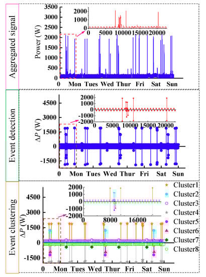
Figure 6.
Results of event detection and clustering for House 2.
Figure 6 illustrates that the significant changes from aggregated power data can be detected accurately using the steady-state segment based on event detection method. After processing all events with the proposed clustering method, eight different clusters were formed, including three “positive” clusters and five “negative” clusters. It can be seen that the elements in each cluster had similar power value.
Table 3 shows the effective detection rate of monitoring events of interest to us. From the Table 3, it can be seen that the proposed algorithm can detect the events effectively.
Table 3.
The effective detection rate of the proposed algorithm.
4.2. Event Pairing
Each positive cluster is matched to the magnitude-wise closest negative cluster according to cluster pairing method. Then for each cluster pair, the forward-backward pairing approach is adopted to search all matching events and reject the unmatched events. Repeat the above process through the remaining unmatched events, until no events can be matched. In iteration, the positive-negative cluster pairs completed the matching process will be stored as the ON/OFF models. When all ON/OFF models are established, we remove them from the set of events and attempt to establish FSM models from the remaining events. Figure 7 presents the results of building appliance candidate models. Four ON/OFF models and one FSM model are established, and their corresponding time profile features are shown in Figure 7. Although the power values of model 3 and 4 are close, they can still be separated due to the large difference in the ON interval.
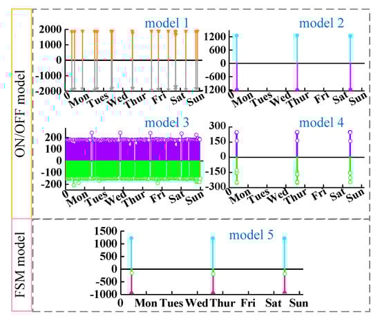
Figure 7.
Results of event pairing for House 2.
The detailed results of the pairing are calculated and shown in Table 4. We can see that the positive and negative power are very close, which proves that the proposed algorithm has good performance in event pairing.
Table 4.
The pairing result of the ON/OFF model 1.
4.3. Load Labeling and Identification
The linear discriminant classifier group of House 2 is used to label each candidate model and the results of each classifier are reported in Table 5. The classifier group of House 2 consists of seven typical appliances with great adjustable potential, including kitchen outlets, stove, microwave, high-power state of dishwasher, low-power state of dishwasher, multi-state of dishwasher and refrigerator. In particular, different modes of dishwasher with different operation cycles are treated as separated appliances. As can be seen in Table 5, the models that are identified as appliance 4, 5 and 6 are all labeled as a dishwasher. From the signs of classifier value (greater than 0), model 1 is determined as appliance 3 while model 2 is appliance 4. Model 3 and model 4 and model 5 represent appliance 7, appliance 5 and appliance 6. If there is no positive value for a model, it means that the model is caused by an unregistered appliance in the feature database, which may be a new or low power consumption appliance not interested by users.
Table 5.
Identification results of separated candidate models.
For the detailed comparison between the disaggregated models and corresponding appliances, the power consumption of each model is reconstructed. The essence is to transform a predicted label into predictive power consumption. The actual and reconstructed power profiles of each appliance are illustrated in Figure 8. The three figures on the left show the power comparison in one day. It can be seen that the algorithm can accurately identify the operation state of each appliance. The power profiles within an interval are displayed on the right side. For the single-state load such as microwave, the power signal can be estimated quite accurately.
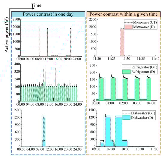
Figure 8.
Ground truth (GT) and estimated appliances’ power consumption (D) for House 2.
To comprehensively verify the effectiveness of the proposed algorithm, the PCEC values are shown in a schematic pie plot. The results of Houses 1, 2, 6 during one week are presented in Figure 9, which illustrates that some appliances in the feature database are OFF during the whole period and the proposed algorithm can detect this pattern accurately. Likewise, there is not any missing identification of an appliance being OFF shown in the disaggregation result. The PCEC values estimated by our method are closer to the ground truth, which further verifies the ability of the proposed algorithm in signal reconstruction. For the three houses, the average absolute differences between the results and the actually measured values are 3.97%, 0.30% and 0.73%, respectively.
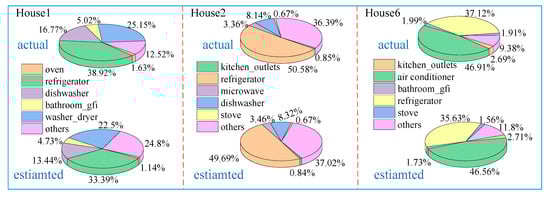
Figure 9.
Comparison of actual and estimated percentage of contribution in energy consumption (PCEC) values for House 1, 2, 6.
4.4. Performance Comparison of Algorithms
In this section, the performance of proposed classification algorithm is compared with some existing algorithms by the parameters of precision, recall and F-measure.
In order to calculate the classification accuracy, the results of the proposed algorithm and unsupervised GSP-based approach [31] on house 1, 2 and 6 are represented in Table 6. It demonstrates that the proposed method has better performance in classification accuracy compared with GSP-based method for all houses.
Table 6.
Classification performance comparison with graph signal processing (GSP)-based method for Houses 1, 2, 6.
Furthermore, the performance of proposed MFIC algorithm is compared with the state-of-the-art NILM approaches used for low sampling rate and power signals. The F-measure values of MFIC, the combined k-means/SVM classification [35], the HMM-based method and the decision tree (DT) approach [17] are denoted as FU, FS, FH, and FDT, respectively. The comparison results are shown in Table 7.
Table 7.
Comparison of four low-rate NILM algorithms using the REDD database.
On the one hand, we study the variation of performance with respect to different appliances, mainly including some controllable or high-power loads in the REDD database. It can be seen that the MFIC algorithm achieves the best disaggregation in terms of F-measure for all appliances. HMM yields significantly have worse results, but it usually performs well in identifying refrigerator because the continuity and singleness (i.e., no other devices operates, especially at night) of its operation bring sufficient data for training. The results of k-means/SVM and DT perform better but worse than those of MFIC. On the other hand, the average results for three REDD houses are compared. The results of combined k-means/SVM classification and HMM are shown in [31], and the results of DT are reported in [36]. The proposed MFIC algorithm has consistently high performance across all three houses and outperforms other algorithms in both House 1 and House 2. The combined k-means/SVM method shows a higher accuracy in House 6.
Moreover, we use the disaggregation accuracy metric to compare the performance of MFIC algorithm with the Bayesian HMM [21], segmented integer quadratic constraint programming (SIQCP) [23], sparse coding (SC), and discriminating sparse coding (discSC) [25]. The comparison results are given in Table 8. Obviously, the MFIC algorithm is improved significantly compared with the SC-based method from previous work and is superior to the Bayesian HSMM model and SIQCP solver, with the disaggregation accuracy increased by 11.1% and 7.1%.
Table 8.
Disaggregation accuracy comparison with other methods.
In addition, we compare with the latest NILM method based on random forest [6] by processing the low-frequency data set of REDD. The comparison results are shown in the Table 9. The random forest method is to use electrical features as training data and adopt random forest method to disaggregation. From the comparison, we can see that the proposed MFIC algorithm performs better in disaggregation. It can disaggregate various loads more accurately.
Table 9.
Comparison of existing NILM algorithms and proposed algorithm.
5. Conclusions
In this paper, a MFIC load disaggregation method is presented, where the only input is the time-stamped power readings from the smart meter. In order to meet the load-monitoring requirements of demand response and energy conservation, the load space to be monitored is narrowed down to some controllable and high-power consumption loads. The system uses a steady-state segmentation-based algorithm to detect events and combines multidimensional features, both electrical and non-electrical, to improve the accuracy of load identification. As the experimental results demonstrated, the linear discriminant classifier group gives excellent classification performance and correctly identifies the devices presented in the load space. Compared with existing NILM approaches, the separation accuracy of the MFIC algorithm is significantly improved due to the reduced load space. Meanwhile, for some loads with similar power, our algorithm can still correctly separate them from aggregate signals.
In future work, we will introduce a machine learning algorithm to further study the adaptive adjustment of load weight parameters. More accurate load models will be established to further improve the accuracy of load identification.
Author Contributions
J.Y. and Y.G. conceived and designed the experiments; J.Y. and Y.W. performed the simulation and analyzed the results; and J.Y. and D.J. wrote the paper; Y.G. and C.S. optimized results and revised the paper; X.W. optimized the method and provided funding support.
Funding
This research was funded by [the Fundamental Research Funds for the Central Universities of China] grant number [2018MS001].
Conflicts of Interest
The authors declare no conflict of interest.
References
- Jung, S.; Yoon, Y.T. Optimal Operating Schedule for Energy Storage System: Focusing on Efficient Energy Management for Microgrid. Processes 2019, 7, 80. [Google Scholar] [CrossRef]
- Lin, Y.H.; Hu, Y.C. Electrical Energy Management Based on a Hybrid Artificial Neural Network-Particle Swarm Optimization-Integrated Two-Stage Non-Intrusive Load Monitoring Process in Smart Homes. Processes 2018, 6, 236. [Google Scholar] [CrossRef]
- Hart, G.W. Nonintrusive appliance load monitoring. Proc. IEEE 1992, 80, 1870–1891. [Google Scholar] [CrossRef]
- Non-Intrusive Load Monitoring (NILM): Combining Multiple Distinct Electrical Features and Unsupervised Machine Learning Techniques. Available online: https://duepublico2.uni-due.de/servlets/MCRFileNodeServlet/duepublico_derivate_00045824/Diss_Bernard.pdf (accessed on 19 June 2019).
- Dinesh, C.; Nettasinghe, B.W.; Godaliyadda, R.I.; Ekanayake, M.P.B.; Ekanayake, J.; Wijayakulasooriya, J.V. Residential appliance identification based on spectral information of low frequency smart meter measurements. IEEE Trans. Smart Grid 2016, 7, 2781–2792. [Google Scholar] [CrossRef]
- Wu, X.; Gao, Y.C.; Jiao, D. Multi-Label Classification Based on Random Forest Algorithm for Non-Intrusive Load Monitoring System. Processes 2019, 7, 337. [Google Scholar] [CrossRef]
- Liang, J.; Ng, S.K.; Kendall, G.; Cheng, J.W.M. Load signature study—part I: basic concept, structure and methodology. IEEE Trans. Power Deliv. 2010, 25, 551–560. [Google Scholar] [CrossRef]
- Hassan, T.; Javed, F.; Arshad, N. An empirical investigation of V-I trajectory based load signatures for non-intrusive load monitoring. IEEE Trans. Smart Grid 2014, 5, 870–878. [Google Scholar] [CrossRef]
- Du, L.; He, D.; Harley, R.G.; Habetler, T.G. Electric load classification by binary voltage–current trajectory mapping. IEEE Trans. Smart Grid 2016, 7, 358–365. [Google Scholar] [CrossRef]
- Wang, L.; Chen, X.; Wang, G. Non-intrusive load monitoring algorithm based on features of V-I trajectory. Electr. Power Syst. Res. 2018, 157, 134–144. [Google Scholar] [CrossRef]
- Huang, T.D.; Wang, W.S.; Lian, K.L. A new power signature for nonintrusive appliance load monitoring. IEEE Trans. Smart Grid 2015, 6, 1994–1995. [Google Scholar] [CrossRef]
- Tabatabaei, S.M.; Dick, S.; Xu, W. Towards non-intrusive load monitoring via multi-label classification. IEEE Trans. Smart Grid 2017, 8, 26–40. [Google Scholar] [CrossRef]
- Gillis, J.M.; Alshareef, S.M.; Morsi, W.G. Nonintrusive load monitoring using wavelet design and machine learning. IEEE Trans. Smart Grid 2016, 7, 320–328. [Google Scholar] [CrossRef]
- Le, T.T.H.; Kim, H. Non-Intrusive Load Monitoring Based on Novel Transient Signal in Household Appliances with Low Sampling Rate. Energies 2018, 11, 3409. [Google Scholar] [CrossRef]
- Guo, Z.; Wang, Z.J.; Kashani, A. Home appliance load modeling from aggregated smart meter data. IEEE Trans. Power Syst. 2015, 30, 254–262. [Google Scholar] [CrossRef]
- Anderson, K.D.; Berges, M.E.; Ocneanu, A.; Benitez, D.; Moura, J.M.F. Event detection for Non-intrusive load monitoring. In Proceedings of the IECON 2012 38th Annual Conference on IEEE Industrial Electronics Society, Montreal, QC, Canada, 25–28 October 2012. [Google Scholar]
- Chang, H.H.; Lian, K.L.; Su, Y.C.; Lee, W.J. Power-spectrum-based wavelet transform for nonintrusive demand monitoring and load identification. IEEE Trans. Ind. Appl. 2014, 50, 2081–2089. [Google Scholar] [CrossRef]
- Makonin, S.; Popowich, F.; Bajić, I.V.; Gill, B.; Bartram, L. Exploiting HMM sparsity to perform online real-time nonintrusive load monitoring. IEEE Trans. Smart Grid 2016, 7, 2575–2585. [Google Scholar] [CrossRef]
- Aiad, M.; Lee, P.H. Non-intrusive load dis-aggregation with adaptive estimations of devices main power effects and two-way interactions. Energy Build. 2016, 130, 131–139. [Google Scholar] [CrossRef]
- Kim, H.; Marwah, M.; Arlitt, M.F.; Lyon, G.; Han, J. Unsupervised dis-aggregation of low frequency power measurements. In Proceedings of the Eleventh SIAM International Conference on Data Mining, Mesa, AZ, USA, 28–30 April 2011. [Google Scholar]
- Johnson, M.J.; Willsky, A.S. Bayesian nonparametric hidden semi-Markov models. J. Mach. Learn. Res. 2013, 14, 673–701. [Google Scholar]
- Kong, W.; Dong, Z.Y.; Ma, J.; Hill, D.J.; Zhao, J.H.; Luo, F.J. An extensible approach for non-intrusive load dis-aggregation with smart meter data. IEEE Trans. Smart Grid 2018, 9, 3362–3372. [Google Scholar] [CrossRef]
- Yuan, Q.; Wang, H.; Wu, B.; Song, Y.; Wang, H. A Fusion Load Disaggregation Method Based on Clustering Algorithm and Support Vector Regression Optimization for Low Sampling Data. Future Internet 2019, 11, 51. [Google Scholar] [CrossRef]
- Kolter, J.Z.; Batra, S.; Ng, A.Y. Energy disaggregation via discriminative sparse coding. In Proceedings of the 24th Annual Conference on Neural Information Processing Systems 2010, Vancouver, BC, Canada, 6–9 December 2010. [Google Scholar]
- Singh, S.; Majumdar, A. Deep sparse coding for non-intrusive load monitoring. IEEE Trans. Smart Grid 2018, 9, 4669–4678. [Google Scholar] [CrossRef]
- Kelly, J.; Knottenbelt, W. Neural NILM: Deep neural networks applied to energy disaggregation. In Proceedings of the 2nd ACM International Conference on Embedded Systems For Energy-Efficient Built Environments, Seoul, Korea, 4–5 November 2015. [Google Scholar]
- Khandelwal, T.; Rajwanshi, K.; Bharadwaj, P.; Garani, S.S.; Sundaresan, R.S. Exploiting appliance state constraints to improve appliance state detection. In Proceedings of the ACM International Conference Future Energy System, Shatin, Hong Kong, China, 16–19 May 2017; pp. 111–120. [Google Scholar]
- Basu, K.; Debusschere, V.; Bacha, S.; Manulik, U.; Bondyopadhyay, S. Nonintrusive load monitoring: A temporal multi-label classification approach. IEEE Trans. Ind. Inform. 2014, 11, 262–270. [Google Scholar] [CrossRef]
- Yang, C.C.; Soh, C.S.; Yap, V.V. A systematic approach in appliance disaggregation using k-nearest neighbours and naive Bayes classifiers for energy efficiency. Energy Effic. 2018, 11, 239–259. [Google Scholar] [CrossRef]
- Henao, N.; Agbossou, K.; Kelouwani, S.; Dube, Y.; Fournier, M. Approach in nonintrusive type I load monitoring using subtractive clustering. IEEE Trans. Smart Grid 2017, 8, 812–821. [Google Scholar] [CrossRef]
- Zhao, B.; Stankovic, L.; Stankovic, V. On a training-less solution for non-intrusive appliance load monitoring using graph signal processing. IEEE Access 2016, 4, 1784–1799. [Google Scholar] [CrossRef]
- Qi, B.; Liu, L.; Wu, X. Low-Rate Non-Intrusive Load Disaggregation with Graph Shift Quadratic Form Constraint. Appl. Sci. Basel 2018, 8, 554. [Google Scholar] [CrossRef]
- Altrabalsi, H.; Liao, J.; Stankovic, L.; Stankovic, V. A low-complexity energy disaggregation method: Performance and robustness. In Proceedings of the IEEE Symposium Computational Intelligence Application Smart Grid, Orlando, FL, USA, 9–12 December 2014. [Google Scholar]
- Marceau, M.L.; Zmeureanu, R. Nonintrusive load disaggregation computer program to estimate the energy consumption of major end uses in residential buildings. Energy Convers. Manag. 2000, 41, 1389–1403. [Google Scholar] [CrossRef]
- Kolter, J.Z.; Johnson, M.J. REDD: A public data set for energy disaggregation research. In Proceedings of the 2011 SustKDD Workshop Data Mining Application Sustainability, San Diego, CA, USA, 21 August 2011. [Google Scholar]
- Liao, J.; Elafoudi, G.; Stankovic, L.; Stankovic, V. Non-intrusive appliance load monitoring using low-resolution smart meter data. In Proceedings of the IEEE International Conference Smart Grid Communications, Venice, Italy, 3–6 November 2014. [Google Scholar]
© 2019 by the authors. Licensee MDPI, Basel, Switzerland. This article is an open access article distributed under the terms and conditions of the Creative Commons Attribution (CC BY) license (http://creativecommons.org/licenses/by/4.0/).