1. Introduction
Sustainable development and controlling climate change can only be achieved with a safe and low-emission energy system. Its transformation involves, i.a., decarbonization of buildings responsible for approximately 36% of all CO
2 emissions in the European Union. Around 40% of the consumption of final energy is spent on heating and cooling, from which most is used in buildings [
1]. This sector is treated as pivotal in accelerating the reduction of emissions of the energy system. It is also a strategic industry in the context of energy safety, since according to the forecasts, till 2030, heating and cooling will account for about 40% of the consumption of renewable energy sources.
Creating smart buildings and cities aims to improve the quality of life of their inhabitants and the protection of the natural environment. As mentioned in [
2], smart grids and smart buildings feature optimized asset management, increase operational efficiency, ensure stable power supply, allow for real-time monitoring of system operation, or enhance the network’s reconfiguration and self-healing ability. The application of smart meters enables a regular monitoring of power consumption and provides access to flexible rates [
3]. Consequently, advanced heating systems can adjust heat supplies to weather conditions and contribute to reducing energy grid losses and emissions.
On the other hand, a high number of connected meters and other IoT (Internet of Things) devices installed in smart buildings, as well as a significant amount of generated data create a challenge for the operators and maintainers. The impact of smart meters and their reliability on the safety of buildings and cities is growing [
4] and therefore requires further study.
Heat meters are used in central heating systems to calculate the consumed energy both in multifamily houses and single apartments or offices. Smart heat meters ensure that costs are settled based on the actual consumption and contribute to saving heat by inhabitants and reducing emissions, particularly in buildings with many tenants.
Currently, as we found, approximately half of the heat meters installed in Switzerland are read manually. However, the number of meters read remotely, which belong to smart meters, increases year by year in Europe [
5]. Recording heat consumption with the use of a smart meter can take place in one-hour intervals or even shorter. The information on the meter state can be directly sent to the operator, thanks to which it is possible to monitor and manage the network regularly.
It is necessary to develop a uniform communication system to introduce the IoT technology for the billing of media and enable the delivery of telemetric data to one node. To ensure the interoperability of connected meters, the OMS (Open Metering System) group [
6] was created in 2015 as a non-profit European organization gathering the leading meter manufacturers and operators. They are working on the standardization of smart meters (not only electricity meters) and a common communication protocol.
Furthermore, the EU directive from 2012 with amendments from 2018 requires that by 25 October 2020, newly-installed heat meters and heat cost allocators should be remotely readable to ensure cost-effectiveness and frequent provision of consumption information [
7,
8]. According to Article 9 of this document, all Member States should implement intelligent metering systems and smart meters, only if it is technically possible, financially reasonable, and proportionate in relation to the potential energy savings.
The reliability of smart meters has a fundamental significance for heat distributors and consumers, since the quality of collected data, the correctness of billing of heat, and making proper decisions in managing heat distribution network depend on it. Unfortunately, studies on the smart meters’ reliability are scarce, and most of the published papers focus on electricity meters and the prediction of power consumption, e.g., [
9,
10] described a non-intrusive load monitoring (NILM) algorithm to provide customers with the breakdown of their energy consumption.
The problem of meters’ reliability and failure prediction was addressed by Khairalla et al. [
4], who proposed a fault location algorithm based on upgrading distribution substation smart meters with synchrophasor measurements. The main downside of this solution was that it required a substantial integration in the existing infrastructure. The reliability of Smart Electricity Meters (SEM) was also analyzed in article [
11], where a linear regression model was used to predict their time-to-failure.
A smart metering technology and harnessing smart meter datasets with a big data approach were presented in the comprehensive review [
12]. Advanced Metering Infrastructure (AMI) data were categorized as consumption and event data. The authors claimed that although the analytic techniques in use were not novel, the volume, velocity, and variance of the AMI collected data enabled applications such as load profiling, forecasting, intelligent pricing, and capturing irregularities.
The importance of smart meter data analytics (including data acquisition, transmission, processing, and interpretation) was emphasized in survey [
13]. Although the authors focused mainly on electricity meters, their comments applied to other types of smart devices, as well. The paper presented a list of widely-used methods and tools; among others, SVM and PCA, which are also used here (
Section 2.4). Unfortunately, failure prediction or reliability analysis was overlooked.
In smart cities, it is of utmost importance to create a prediction system, thanks to which the operation of the heat distribution network is well adjusted to the needs of recipients. There are several examples of using ML algorithms in the context of smart buildings and smart heat meters, usually ANN, for maintaining a comfortable indoor environment [
14,
15]. Although such an approach is effective, it has a significant disadvantage: a new, unique ANN has to be built for every single apartment and tenant. However, to manage and control large heating systems in smart cities, more general and robust models are necessary.
The studies on the optimization of the heating system in residential buildings were also presented in paper [
16], where an optimized ANN model determined the optimal start time for a heating system in a building. Similarly, an ANN was applied in [
17] to evaluate the energy input, losses, output, efficiency, and economic optimization of a geothermal district heating system.
In district heating systems, multi-step ahead predictive ML models of individual consumers’ heat load could be a starting point for creating a successful strategy for predicting the overall heat consumption [
18]. As a consequence, transfer losses, costs of heat purchase, and pumping costs can be reduced. Facilitating the measuring system is associated with the improvement of the efficiency of communication with distributed sensors, remote control, and monitoring of technological processes.
Hyperparameter optimization is a relatively new concept in the ML world. Its usefulness was confirmed for example in [
19]. The authors compared Tree of Parzen Estimators (TPE) with the random search strategy. Prepared experiments showed that TPE clearly outstripped random search in terms of optimization efficiency. TPE found best-known configurations for each dataset and did so in only a small fraction of the time allocated to random search. That is why a TPE approach is followed in this paper. The general Sequential Model-Based Optimization (SMBO) method used for hyperparameter optimization (
Section 2.4) is in line with a procedure described by Bergstra et al. [
20], however adapted to the selected ML algorithms.
In contrast to hyperparameter optimization, the ensemble classifier has enjoyed growing attention within the computational intelligence and machine learning community over the last couple of decades. This rather simple idea was deeply explained in [
21]. The author emphasized the importance of diversity in ensembles. Ideally, classifier outputs should be independent. Although diversity can be achieved through several strategies, usage of different subsets of the training data is the most common approach. Another less common approach also included using different parameters of the base classifier (such as training an ensemble of multilayer perceptrons, each with a different number of hidden layer nodes) or even using different base classifiers as the ensemble members. In this paper, we use the latter, which ensures the greatest diversity.
2. Materials and Methods
2.1. Heat Meters
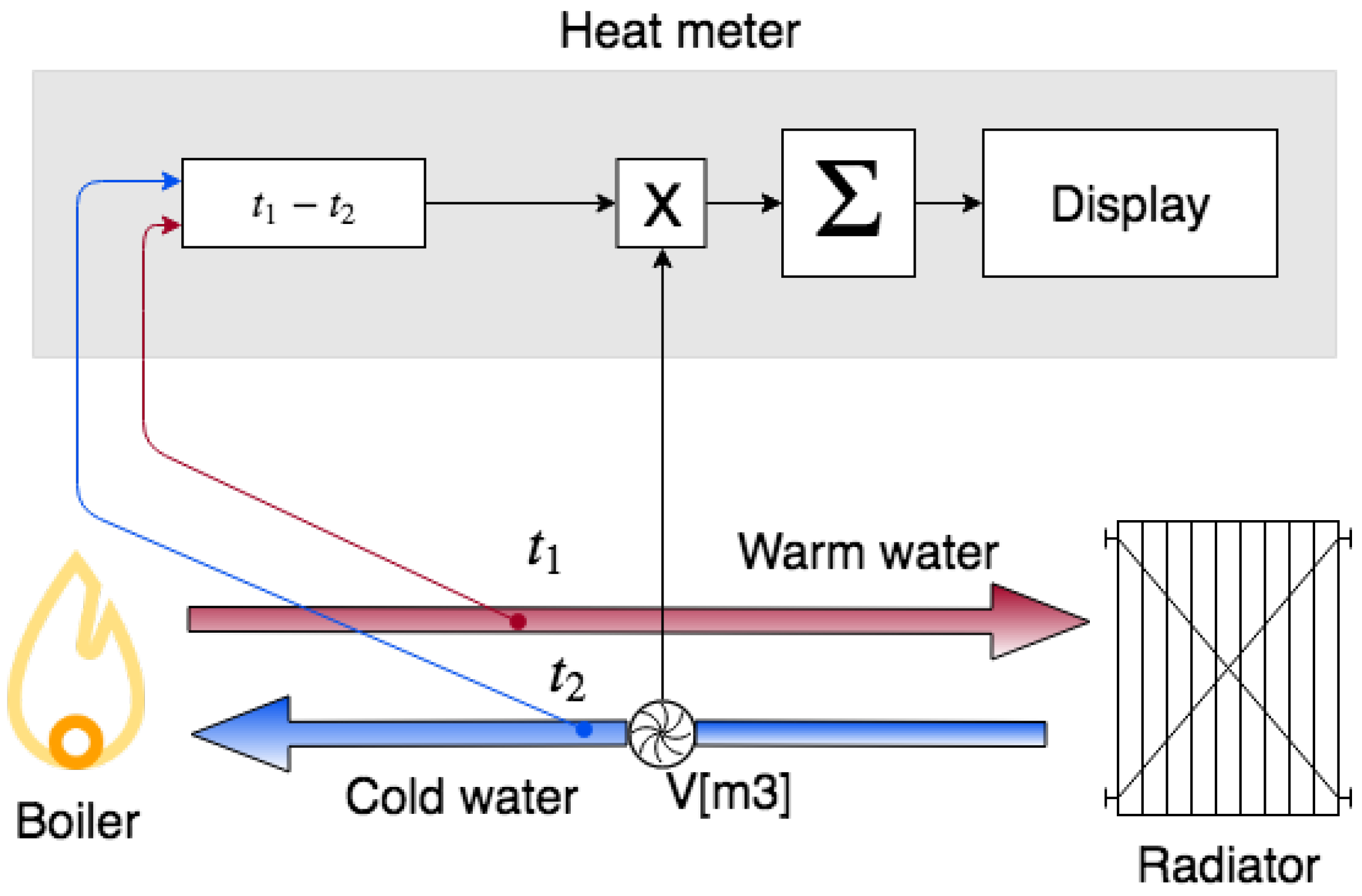
A heat meter is a microprocessor-measuring device that calculates the consumption of heat in kWh by measuring the flow rate of the heat transfer medium (most often it is water, although if the system is also used for cooling, it can be water with appropriate additives to prevent freezing) and the difference between supply and return temperature (
Figure 1). The meter has an in-built flow meter, which measures the volume of the flowing medium, and two temperature sensors for the inflow and outflow fluid.
Temperature sensors consist of a measuring element, that is a thermistor, which is usually platinum. It changes resistance depending on the temperature. In heat meters, usually Pt100 or Pt500 sensors are used. The higher the resistance of platinum in the sensor (respectively 100 or 500 ), the greater the accuracy of temperature measurement.
2.1.1. Maintenance of Heat Meters
Heat meters are generally considered as reliable. However, like all devices, they sometimes break down and require technical maintenance. Premature meter failures affect all parties, i.a., tenants, building managers, and the billing company, significantly disturbing the scheduled maintenance and causing losses. The consequences include incorrect readings, understated invoices, and customer complaints.
The replacement of meters is a complex logistical process, which must be planned in detail. The old meters have to be removed from the network and delivered to a service center or recycled. The installation of new meters is usually done in stages, and it is convenient to carry out the service works in a limited area before proceeding to the next one. It is necessary to arrange meetings with building managers or tenants.
The whole procedure can generate high costs related to the work of qualified installers, planning and delivering of components, final inspection of the installed devices, and updating the operational data regarding meters. It is often more efficient to replace a functioning device during a scheduled maintenance check if there are any indications of a possible failure in the next billing period. Developing a method for predicting the occurrence of the meter failure in the subsequent period is the subject of this article.
Heat meters are as a rule the subject of planned maintenance. In the majority of the European countries, their verification should take place every five years due to metrological requirements. During this time, heat meters accumulate mineral deposits from water (especially warm and hot), which results in wear of mechanical elements due to being moved by the stream flowing through the equipment. To mitigate this problem, regular checks are done, aimed at investigating the quality of water used for heating.
Reverification is time consuming. Heat meters have to be dismounted from the network and delivered to the verification point. For the verification period, the older heat meters are replaced with the new ones, which have a valid heat meter verification marking. However, currently, the majority of the companies plan only one verification visit due to logistical costs. Once the verification is done, the dismounted heat meters are installed in other locations. Before the verification, the heat meters are cleaned, regulated, and sealed so that they could work for another five years, meeting metrological requirements. It is not uncommon that heat meters are verified two or even three times.
The users decide to replace them due to three reasons: new equipment has a longer warranty than the older verified one (five years instead of two years); the new heat meter is much more technologically advanced; or the old heat meter was broken, and repair is impossible or useless.
2.1.2. Review of Typical Faults
The most common causes of meters’ failures include:
Failure of the flow transducer (in a mechanical meter) caused by the accumulation of deposits on mechanical elements. The repair involves exchanging the rotor or the whole transducer.
Failure of temperature meter: Most frequently, this occurs in non-mechanical heat meters and is usually caused by rodents (rats) damaging the conductors. The repair is based on the replacement of the temperature meter.
Exhaustion of the battery: Despite the theoretical calculations that mounted batteries should work for 5–7 years (exceeding the required verification period), it frequently happens that the batteries run out already after 2–3 years. The repair of such equipment requires only the replacement of the battery.
2.2. Data
Information on installation, operation, and replacement of heat meters has been accumulated over the last ten years in a relational database. The meter is a subject of a cyclical readout of its current value necessary to calculate the energy consumption in a defined billing period. Potential failure should be detected at the latest at the time of meter readout. The billing period usually lasts 12 months (but it can also last 6, 18, or 24 months) and starts at the beginning of the chosen month (often it is January, June, or September). Some modern smart meters also store the monthly values, although they do not impact the final billing.
The discussed database also includes many other items of information used for the billing of utilities (approximately 150 relational tables; some of them consist of 20 million records; in total, 250 GB of data), as well as data regarding other types of meters (water meters and heat distributors). However, the authors decided to focus on the heat meters addressed in the introduction. The available data may offer clues to many questions concerning the operation of heat meters. For economic reasons, the most significant problem is detecting and predicting a failure; thus, the data were prepared for this purpose.
After data preparation and initial statistical analysis, sixteen parameters were selected for further processing (
Table 1).
The type of the usable surface (e.g., flat, office, or storeroom), as well as the type of room (e.g., room, kitchen, bathroom, and corridor) were represented by enumerations. In case of an unclear situation, the value “other” was used. The authors decided to distinguish sixteen types of rooms and five types of usable surfaces. Since some models accept only numbers, each type of room was assigned a successive natural number. The same was done in the case of meters’ manufacturers (16 different values).
The rating factor is a real number from the interval (0–1]. It is used in the case of rooms with an increased consumption of heat, e.g., due to adjacency to external walls of the building. This ensures a fair distribution of the heating costs of the whole building between all tenants, irrespective of the fact of whether they have an external flat or not.
An important parameter is also the method of communication with the equipment (CommType). There are four communication types:
bus: meters regularly send their updates to the central panel installed in the same building, which also collects data from other meters by cable connection;
funk: similar to the bus, but the connection of the meter with the control panel does not require the additional wiring system;
walk by: on specific days (programmed), the meter sends data, which have to be collected by the technician sent to the neighborhood and equipped with the receiving device;
without a module: the reading has to be done manually directly on the meter.
The correction and normalization of the dataset were described in more detail in [
22].
2.3. Data Analysis
Preparation of data and selection of observation parameters theoretically enables building prediction models. In practice, however, it is necessary to better understand data, on which the studies were conducted [
23]. By its very nature, a machine learning model is acutely sensitive to the quality of the data. Because of the huge volume of data required, even relatively small errors in the training data can lead to large-scale errors in the output. Finding and analyzing the relations between particular parameters enables drawing correct conclusions and the proper interpretation of the results [
24]. Apart from this, such knowledge can be useful by selecting the appropriate machine learning model or its parameters [
25].
The code in this project was written in Python, which offers advanced tools for machine learning and data analysis. In order to train and evaluate the selected models, the following components and applications were used:
Python 3.6.3;
Keras 2.2.0: open source library for creating neural networks;
TensorFlow 1.8.0: open source library written by the Google Brain Team for linear algebra and neural networks;
Scikit-learn 0.19.1: open source library implementing many different methods of machine learning.
2.4. Machine Learning Algorithms
The developed ML classifier was aimed to predict meters’ failures in the next billing period. To ensure a high degree of independence, three significantly-different machine learning algorithms were used: SVM (Support Vector Machine) with the RBF kernel, ANN (Artificial Neural Network), and BDT (Bagging Decision Trees) in standard implementations. The underlying theory can be found in [
26,
27,
28,
29,
30].
Next, the general method of hyperparameters’ optimization was employed to improve prediction efficiency. At the end, the optimized SVM, ANN, and BDT models were used to build an ensemble classifier (
Supplementary Materials). The purpose of this procedure was to obtain a model able to make the best prediction concerning the failure rate of meters, while maintaining its generalization, i.e., minimizing overfitting. The Python code of the optimized models, ensemble model and hyperparameter optimisation procedure is available online at:
https://github.com/PatrykPalasz/ML-algorithms-and-hyperparameteroptimisation.git.
For training the selected models, the default parameters of the algorithms were used, as well as all the features of the observations presented in
Table 1. Building and evaluating models were always based on the same dataset (51,890 records), randomly divided into the training set (80%, 41,512 records) and the testing set (20%, 10,378 records).
3. Results and Discussion
3.1. Statistical Analysis
One of the first steps in exploratory research is usually constructing a correlation matrix [
31]. Frequently, its analysis allows eliminating the irrelevant parameters and may be a starting point for PCA analysis. Apart from that, the correlation matrix may reveal some dependencies between particular variables, their mutual relations, and potential redundancies [
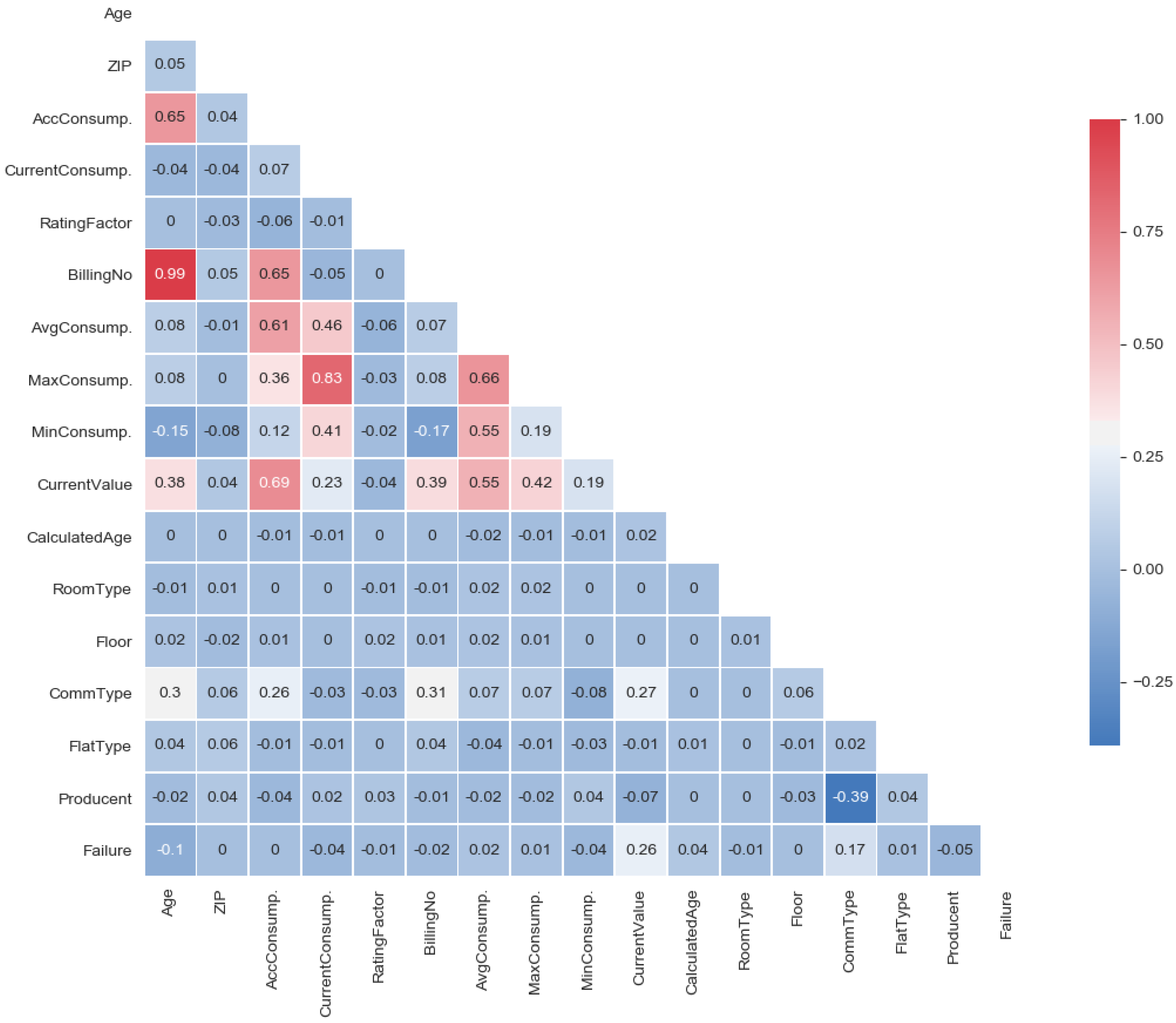
32]. To visualize such information, a thermal map was applied. By analyzing the correlations presented in
Figure 2, a very weak relation of failure from all other parameters (the last row of the matrix) can be observed.
The highest correlation coefficient at had a parameter of a current meter value. Such a correlation value was relatively small and is usually omitted. On this basis, it can be concluded that failures did not directly depend on any single meter feature, but perhaps on some nonlinear combination of state variables.
A very strong correlation can be observed between the meter age and the number of billings (nearly one). Presumably, one of these parameters would be unnecessary (redundant) in further analysis. A little smaller, but also significant correlation can be seen between the maximum and the current energy consumption. Furthermore, this relation was rather apparent and did not require any more explanations.
There were no rows below the current meter value, which demonstrated higher correlation with other parameters and could be treated as linearly independent. Attention is drawn only to the small correlation between the manufacturer and the type of communication, which was at . This indicates the situation where manufacturers specialize themselves in making meters for particular communication types, but also the maintenance company is supplied with particular types of meters not only by the selected manufacturers.
During the analysis of the correlation matrix, it should not be forgotten that a strong correlation does not necessarily imply that correlation is causation.
3.1.1. Communication Type
Because the minimization and predictability of failures was crucial for cost optimization, we examined the dependence of failures on selected parameters. The impact of the meter communication type is presented in
Table 2.
The meters of the “walk by”-type had a very low percentage of failures, but the sample was small in relation to other types of communication, so the conclusion that they were the most reliable was a bit premature. Meters without a communication module failed almost twice as often as those with communication. We can certainly conclude that the meters with remote communication, in other words, the new generation of devices, were far less likely to fail.
Using the methods presented in [
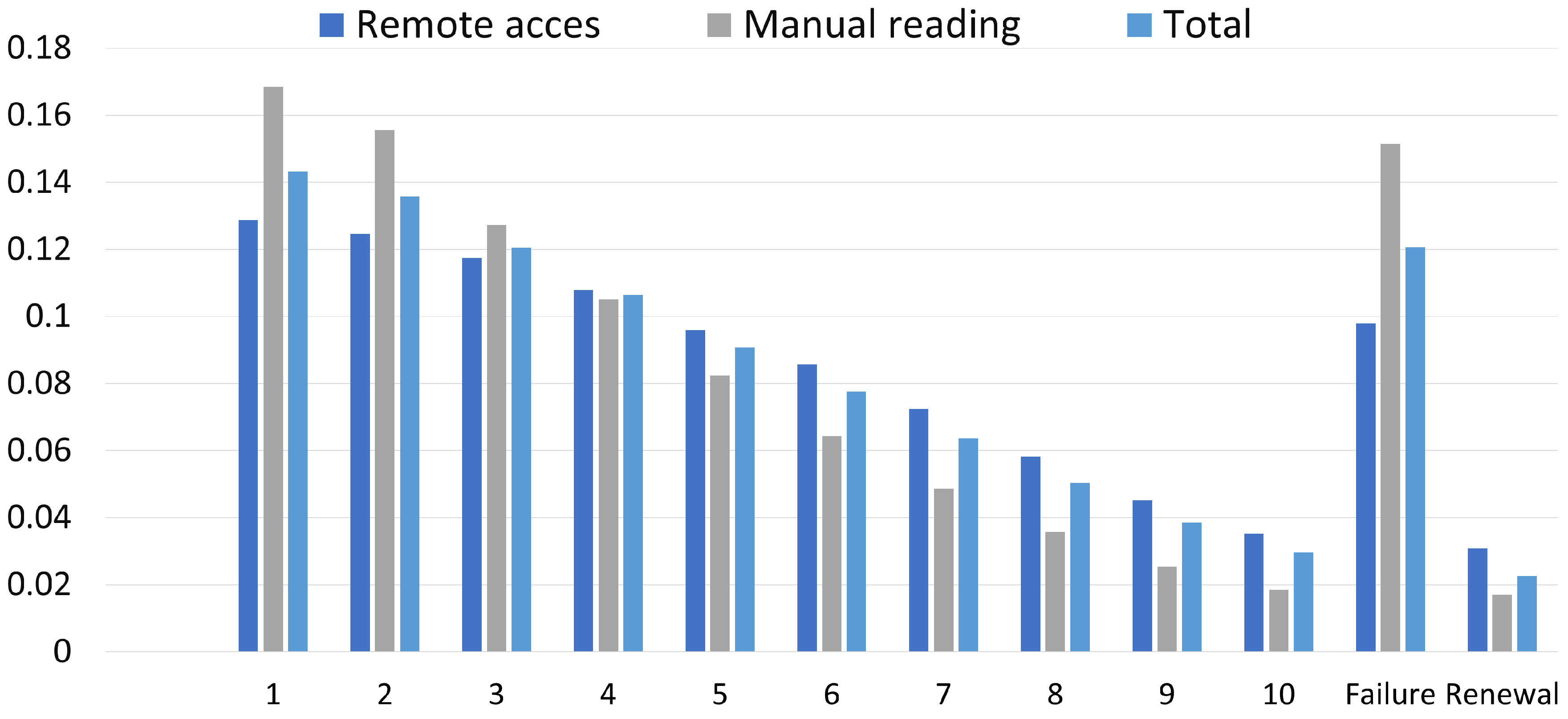
22], the distribution of the probability vector can be determined. In
Figure 3, each state from 1–10 represents the age of the meter in years. It can be observed that there was a significant difference in failures between meters with and without communication, also in the long term. The linearity visible in that figure confirmed that the failure intensity was weakly dependent on the meter’s operating time. Moreover, information about stationary distribution allowed for better planning of inventory.
Therefore, in the context of smart meters and smart buildings, devices with remote reading are definitely a better choice. Not only are they more “user friendly” (the presence of the resident is not required during readings), but also more reliable.
3.1.2. Producer
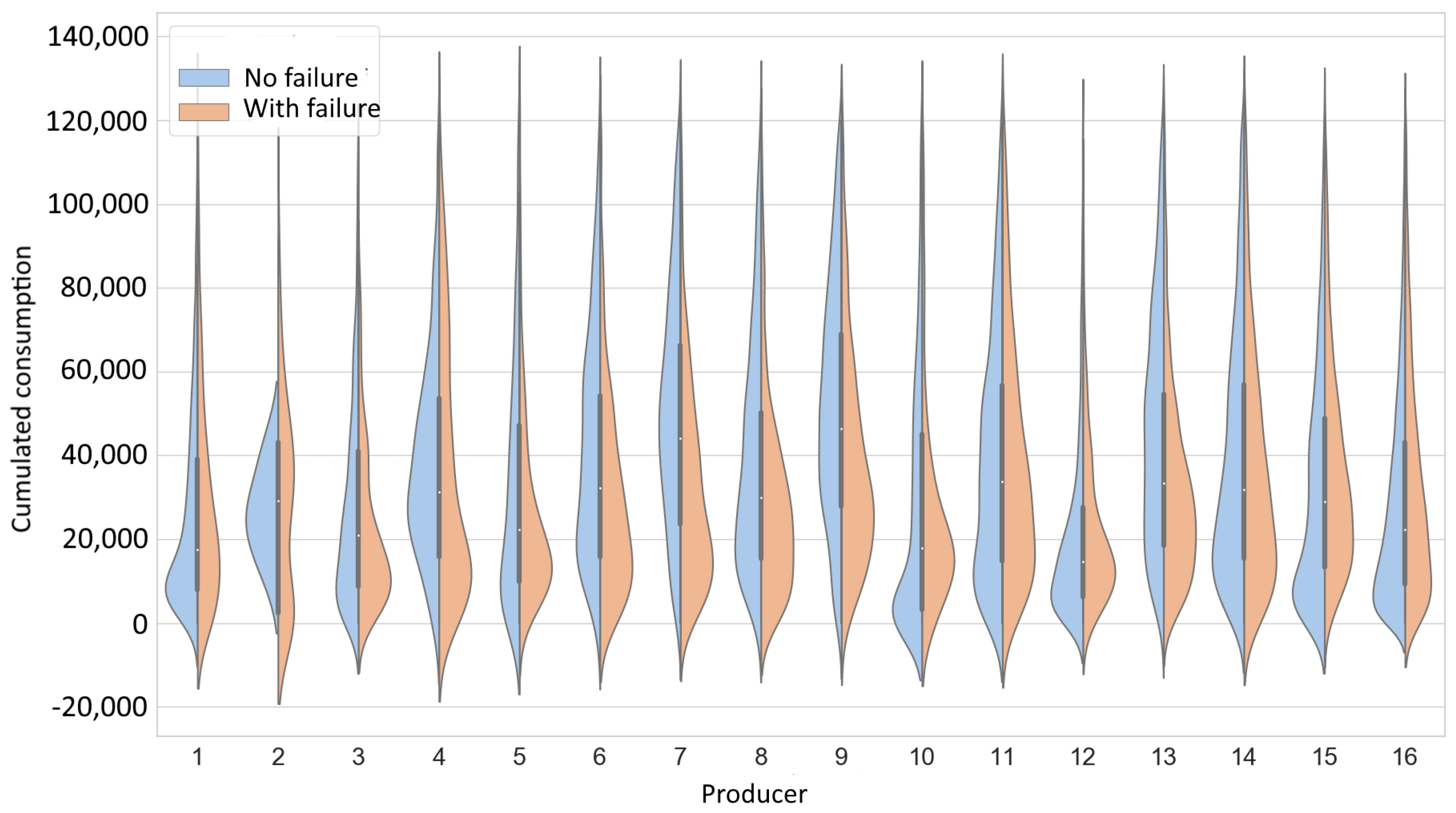
Similarly to the grouping by the type of communication, violin charts with the division into the producers are presented (
Figure 4). Due to the sensitivity of the data, the numbers were used instead of the brand names. Analyzing violin plots, it is worth noting that the curves of the Kernel Density Estimator (KDE) represent the probability density, not the cardinality of the considered set. In other words, the area under the curve equaled 100%. More information about how the KDE was created can be found in [
33]. A single violin in the presented plot describes two sets: left-hand without and right-hand with failures (blue and orange, respectively), which are not in the same scale in terms of absolute numbers. To interpret the data, the locations and number of picks, as well as the shape of the curve itself need to be compared.
In particular, Manufacture Nos. 2 and 4 had their maxima without failure above consumption of 20,000 kWh, which suggests that purchases were abandoned. In the case of Producer No. 10, the failures were slightly delayed in relation to the number of new meters, but it was difficult to draw any more specific conclusions here. It was notable that the KDE curves of failure were in general longer and had relatively small maxima, which indicated that the occurrence of failure was random for almost any manufacturer.
Table 3 is the complement of the violin charts. The failure results presented here were certainly influencing the Rapp’s purchasing policy. On the one hand, we had a strong leader (Producer No. 16), which maintained the failure rate of its devices at a relatively low level of 13%. On the other hand, we observed diversification and an attempt to become independent of this producer. The reason to withdraw the meters of Producer No. 2 was the high failure rate of over 90%, even in a few years.
The above observation strongly supported the thesis that statistical analysis performed on a big dataset can create significant savings and should be used in the process of designing and maintaining smart buildings.
3.2. Reliability Analysis
The cumulative heat consumption is a meter feature, which can be treated as an equivalent of operating time. In article [
22], we showed that the probability of failures follows a Weibull distribution. With the
k parameter close to one, it is simply the exponential distribution:
It is characterized by the constant intensity of failures, i.e.,
=
. This means that failures occur as external random events and do not depend on usage time. Instead, they appear randomly with the fixed intensity. Such a feature is called a “memoryless” of the exponential distribution and implies that if we know that in moment
x the element was fit for use, thus, counting from that moment, the fitness time had the same distribution as a distribution of a new element [
34,
35,
36].
It can be stated that during these ten years, the intensity of failures of the heat meter was weakly dependent on the usage time. It is a fundamental assumption since it enables the prediction of failures, which are independent of the history of operation. We did not have to possess information on how and when the equipment was used; if we know its state variables, it is entirely sufficient. The above conclusion, as well as correlation matrix suggested the selection of algorithms of machine learning that perform well in classification problems with non-linear separable classes.
3.3. Machine Learning
3.3.1. Metrics
There are many different metrics that can be used to compare the performance of trained ML models; each has its strengths and weaknesses (compare [
37,
38]). Due to the character of the data (high predominance of records without failure; approximately 80%), as well as the goal of the model (equally important as predicting failure is predicting whether the meter will continue working), we focused on two metrics: Area Under the ROC Curve (AUC) and Matthews Correlation Coefficient (MCC). The MCC takes values from
(more means better), and AUC takes values from
, whereby
means a random classifier. Detailed information about each of metrics can be found in [
39]. For a more comprehensive image, also accuracy, precision, recall, and
for both classes will be provided.
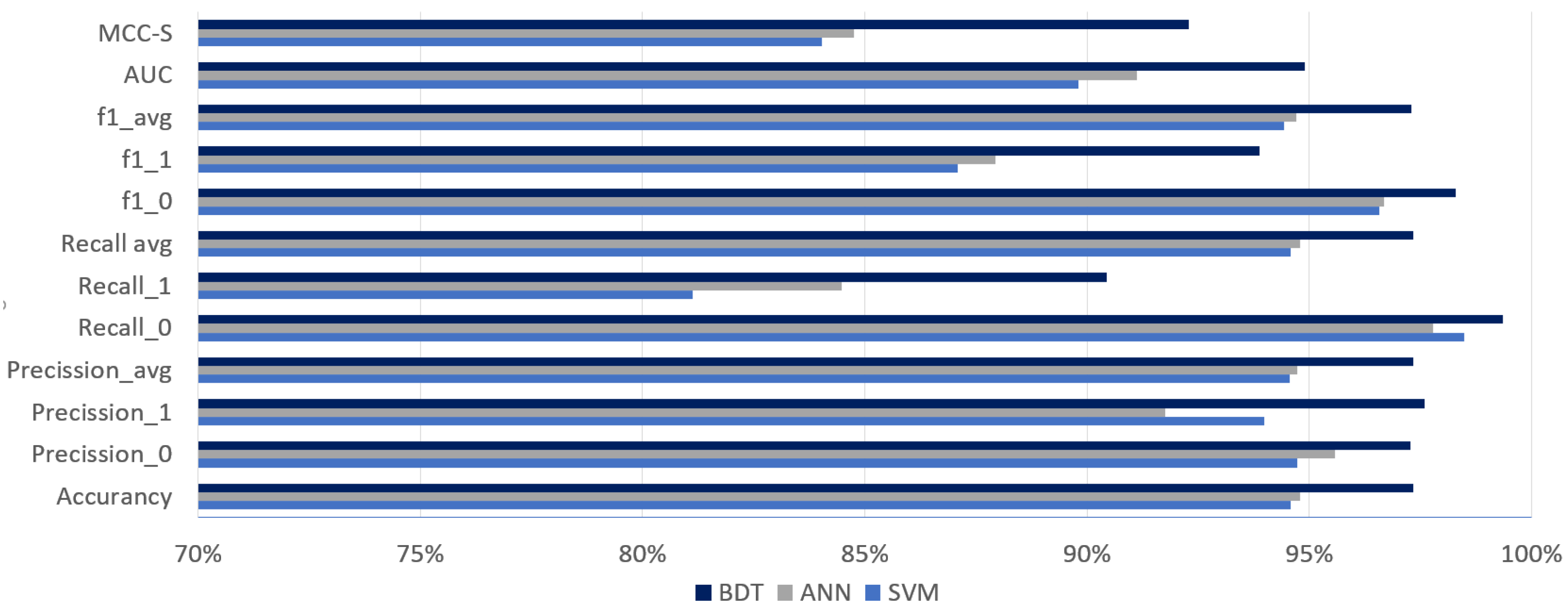
Figure 5 shows the results of the BDT, ANN, and SVM models in various metrics. It can be noted that
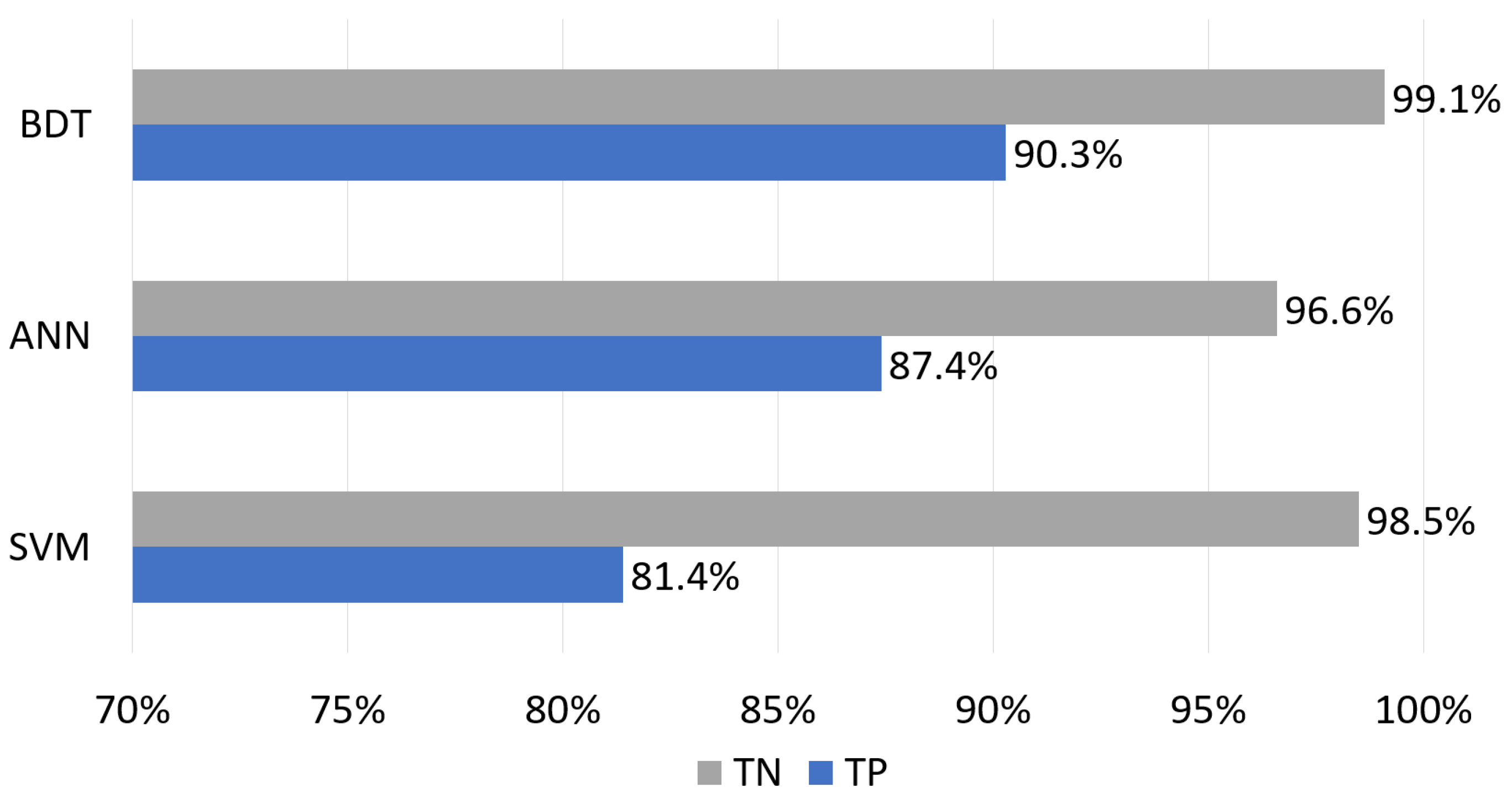
MCC-S and recall for a positive class were relatively weak. This indicated that the developed models were good only for the correct prediction of an event that a meter will not fail, but the correct prediction of breakdown was more challenging. The same conclusion can be reached by analyzing
Figure 6, which presents a part of the confusion matrix regarding true predictions (true positive and true negative). Differences of a few or several percent were more difficult to accept, and their minimization was thus the target of hyperparameter optimization.
As far as the performance of individual algorithms was concerned, BDT turned out to be the best and SVM the worst (
Figure 6). All models were much less successful in detecting meter failure than predicting survival for the next billing period. Although we had not yet optimized the tested models, their overall performance was very good. This resulted mainly from preprocessing and data normalization, as well as the proper selection of parameters.
3.3.2. Hyperparameter Optimization
Hyperparameter optimization is a problem of finding a minimum of a certain objective function, the domain of which is the space of parameters of the examined model. The parameters can be continuous, discrete, or categorical, and additionally, they can be dependent on each other [
19]. It is worth highlighting that calculating the objective function is extremely expensive: it involves the full training and evaluation of the model.
There are different strategies of looking for optimum hyperparameters. The easiest way is “manual” tuning. However, it requires expert knowledge of the model and data, which does not foster generalization. The other strategy is either full or the random search of the parameters’ domain, the so-called “grid search”. Checking all combinations is usually unrealistic due to the high costs. It has been confirmed that random search can work well in the case of a model with many parameters, out of which only some play a key role in its quality [
40]. The next method of searching for optimum parameters of a classifier is an SMBO (Sequential Model-Based Optimization) method. To put it simply, it consists of constructing a surrogate model approximating the objective function, the minimum of which we look for. Most frequently, GP (Gaussian Process), RFR (Random Forest Regressions), or TPE (Tree-structured Parzen Estimator) are used as surrogate models. The selection of subsequent domain points (values of hyperparameters) is calculated in order to optimize the selection function; here, we usually used the EI function (Expected Improvement). Such a strategy often provides the best results and eliminates the element of randomness [
41].
To optimize the hyperparameters of models described in this paper, SMBO with TPE model was chosen. As the objective function, the AUC metrics was applied.
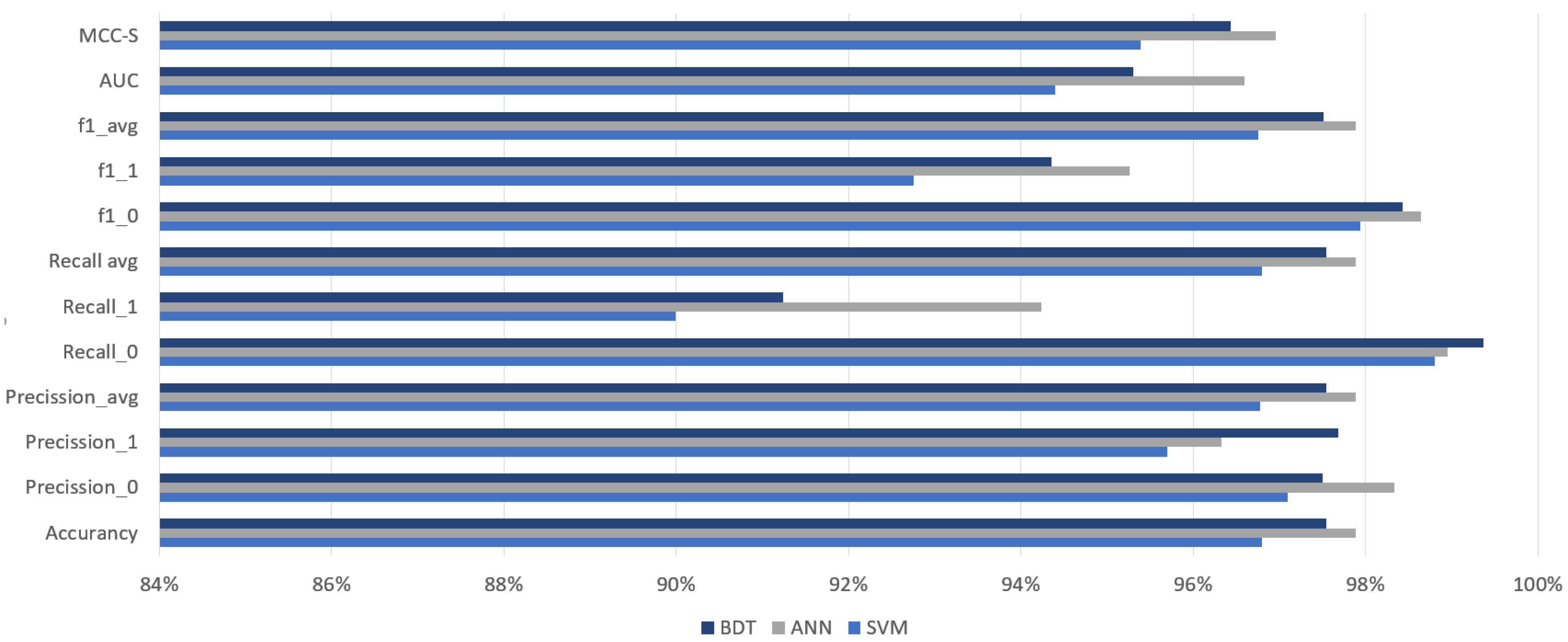
After optimizing the hyperparameters, each of the models improved its performance, especially in failure detection. This was also the main goal of the optimization that was achieved. It can be noticed that the larger the hyperparameters of the tested model, the easier it can be optimized. The neural network noted the highest progress in each metric (compare
Figure 7). Significant progress was also visible in the SVM model.
In general, most of the metrics showed progress in the range of 3–5%, which is a very good result, especially considering that the quality of the examined models before the optimization exceeded 92%.
3.4. Ensemble Model
To increase the efficiency of predictions, an ensemble classifier was built from three independent models: SVM, ANN, and BDT. Similarly, to random forests, an ensemble is a meta-classifier that internally uses several, preferably strongly independent models, respectively aggregating their predictions to generate the result [
42]. The choice of algorithms in that case cannot be accidental. For example, the logistic regression method would be a bad choice because the selected parameters of heat meters are linearly independent (
Figure 2). The assumption about the differentiation of models is important because similar classifiers make the same mistakes, so the final group model would only duplicate them. Sufficient differentiation can be achieved for the same algorithms by the appropriate division of the training set into subsets (bagging). It also happens that subsets of data attributes are used instead of data subsets. In this paper, the authors decided on a different approach, namely the use of already trained (and optimized) models and building of a collective classifier using the most popular voting algorithms with weights. The results of the obtained ensemble classifier can be seen in
Table 4.
For the most important metrics (MCC and AUC), the ensemble classifier was better than the average of the optimized models by more than one percent, which gave 22% and 29%, respectively, of the total possible improvement. The increase in detectability of failures by more than 1.5% for the , , and metrics was also important.
4. Conclusions
It is not possible to replace at once all heat meters currently being in use. Therefore, we need to characterize the existing devices much better to be able to implement the idea of smart buildings. The knowledge needed for data analysis and model building is available to researchers and fairly well established [
43]. Access to large datasets containing information about the operation of already installed devices in residential buildings is currently relatively easy. The analysis of these data (in
Section 3.1 and
Section 3.2) provided significantly new knowledge about their operation. This is as an intermediate step in the implementation of heat meters into smart buildings.
The reliability of heat meters, especially of those with remote communication, seems to be good enough for smart city applications, and optimization of heat consumption (
Figure 3 shows a failure rate around 11%). We discovered that the failure intensity of the heat meters was random and weakly dependent on the time of their use and followed a Weibull distribution (
Section 3.2), which was in line with the studies on electricity meters [
11]. In addition to statistical analysis, a selection of machine learning algorithms, including neural networks and an ensemble model for heat meters’ failure prediction, was implemented.
Currently, most applications of machine learning are primarily based on neural networks. It is understandable that this method is very flexible and probably the only one suitable for solving many types of problems such as regression, classification, clustering, and reinforcement. Consequently, the alternative types of algorithms are rarely considered. We showed that prior exploratory data analysis, the right choice of parameters, hyperparameters’ optimization, and building the ensemble classifier can significantly enhance the quality of predictions and create a solution that outperforms the results of an individual neural network. As studies using hyperparameter optimization are not common, this encouraged us to present this issue a bit more widely. We also showed that this is an important step to improve the efficiency of machine learning models.
The presented data analysis and the results of created models led to the following findings and implications:
The intensity of failures of heat meters was almost independent of the operating time.
Due to the high reliability of the meters and their considerable cost, condition-based or predictive maintenance of heat meters was justified and possible. It was shown in
Section 3.2 that the mandatory five-year verification period could be extended.
Collecting different parameters about devices in use made sense even if they are not required at the moment. This allowed building more general and better ML models in the future.
Heat meter data allowed building a ranking list of their producers and optimize deliveries.
Heat meters with remote communication were twice as reliable as the ones with manual reading.
This article is one of the few that dealt with the reliability and predictability of heat meters’ failures. It is also, according to our knowledge, the first attempt to use more independent ML models based on a single database. Achieving the result above 95% for the AUC metric by the model, while maintaining overfitting at the minimum level, was a remarkable outcome.
As stated in [
24], many ML methods are very sensitive to the type and quality of the data. We selected and prepared the data with extra care to ensure the quality of the classifier, but it is not certain whether equally good efficiency could be achieved for meters and data derived from other sources. Due to the fact that the training data were supplied by only one meters’ operator, the models can be biased. However, the presented approach and methodology of model construction should perform well independent of data sources.
The implemented methodology is so universal that it will be utilised to study the reliability and predict failures of other types of meters, e.g., water meters or heat cost allocators. Besides fault prediction, a similar approach can also be implemented to predict water usage, heat consumption or periods when such consumption is minimal. This knowledge can be used to optimize the costs of media transmission as well as to reduce costs for individual users [
18]. Similar approach was shown in [
44], but it was based on an adaptive neuro-fuzzy network.
The developed machine learning model and the acquired knowledge will be used in the design of new heating systems, as well as for optimization of stocks and maintenance activities in the existing heat meter networks, which will bring significant benefits for their operators, tenants, and the environment. In particular, the optimization of meters’ maintenance in large buildings will allow companies to save both time and resources. Such optimization is also crucial for the tenants, who are the end users of heat meters. It does not only shorten the time needed for their presence during replacement, but it also guarantees the accurate meter readings and fair distribution of heating costs.


