Intelligent Neural Network Schemes for Multi-Class Classification

1
Department of Electrical Engineering, National Sun Yat-Sen University, Kaohsiung 804, Taiwan
2
Department of Electrical Engineering, Intelligent Electronic Commerce Research Center, National Sun Yat-Sen University, Kaohsiung 804, Taiwan
3
Department of Neurology, Graduate Institute of Medicine, Kaohsiung Medical University, Kaohsiung 807, Taiwan
4
Department of Neurology, Kaohsiung Medical University Hospital, Kaohsiung 807, Taiwan
*
Author to whom correspondence should be addressed.
Appl. Sci. 2019, 9(19), 4036; https://doi.org/10.3390/app9194036
Submission received: 31 August 2019
/
Revised: 20 September 2019
/
Accepted: 20 September 2019
/
Published: 26 September 2019
(This article belongs to the Special Issue Intelligent System Innovation)
Abstract
:Featured Application
This work can be used in engineering and information applications.
Abstract
Multi-class classification is a very important technique in engineering applications, e.g., mechanical systems, mechanics and design innovations, applied materials in nanotechnologies, etc. A large amount of research is done for single-label classification where objects are associated with a single category. However, in many application domains, an object can belong to two or more categories, and multi-label classification is needed. Traditionally, statistical methods were used; recently, machine learning techniques, in particular neural networks, have been proposed to solve the multi-class classification problem. In this paper, we develop radial basis function (RBF)-based neural network schemes for single-label and multi-label classification, respectively. The number of hidden nodes and the parameters involved with the basis functions are determined automatically by applying an iterative self-constructing clustering algorithm to the given training dataset, and biases and weights are derived optimally by least squares. Dimensionality reduction techniques are adopted and integrated to help reduce the overfitting problem associated with the RBF networks. Experimental results from benchmark datasets are presented to show the effectiveness of the proposed schemes.
1. Introduction
Classification is one of the most important techniques for solving problems [1,2]. Infinitely many problems can be viewed as classification problems. In daily life, telling a female person from a male one is a classification problem, which is probably one of the earliest problems people face to solve. Giving grades to a class of students could be an uneasy classification task for a teacher to work with. Deciding the disease a patient may have based on the symptoms is a difficult classification task for a doctor. Classification is also useful in engineering applications [3,4,5,6], e.g., mechanical systems, mechanics and design innovations, applied materials in nanotechnologies, etc. For example, classification of structures, systems, and components is very important to safety for fusion applications [7]. The product quality has been found to be influenced by the engineering design, type of materials selected, and the processing technology employed. Therefore, classification of engineering materials and processing techniques is an important aspect of engineering design and analysis [8].
In general, classification consists of two phases, training and testing, as shown in Figure 1. In the training phase, a collection of labeled objects is given. After attribute extraction, a set of training instances is obtained, and they are used to train a model. In the testing phase, the trained model is used to evaluate any input objects to determine which categories the input objects belong to. Normally, there are m categories, , such as Medicine, Finance, History, Management, and Education, involved in the multi-class classification problem [9]. The data to be dealt with can be either single-label or multi-label. If the given object belongs to one category, it is called single-label classification. On the other hand, it is called multi-label classification if the given object can belong to two or more categories [10,11].
In this paper, multi-class classification is concerned with a given set of N training instances,
, where
- , , is the input vector of instance i. There are n attributes, with real attribute values in .
- , is the input vector of instance i. There are m, , categories, category 1, category 2,…, category m. For instance, i, if the instance belongs to category j and if the instance does not belong to category j, .
Note that indicates the k-vector . The aim of this paper is, given the set of N training instances, to decide which categories a given input vector, , belongs to. For single-label classification, one and only one +1 appears in every target vector, while for multi-label classification, two or more entries in any target vector can be allowed to be +1.
Traditionally, statistical methods were used for multi-class classification [12,13]. Recently, machine learning techniques have been proposed for solving the multi-class classification problem. The decision tree (DT) algorithm [14,15] uses a tree structure with if-then rules, running the input values through a series of decisions until it reaches a termination condition. It is highly intuitive, but it can easily overfit the data. Random forest (RandForest) [16] creates an ensemble of decision trees and can reduce the problem of overfitting. The naive Bayesian classifier [2] is a probability-based classifier. It calculates the likelihood that each data point exists in each of the target categories. It is easily implemented but may be sensitive to the characteristics of the attributes involved. The k-Nearest neighbor (KNN) algorithm [17,18,19] classifies each data point by analyzing its nearest neighbors among the training examples. It is intuitive and easily implemented. However, it is computationally intensive.
Neural networks are another machine learning technique, carrying out the classification work by passing the input values through multiple layers of neurons that can perform nonlinear transformations on the data. A neural network derives its computing power mainly through its massively parallel, distributed structure and its ability of learning and generalization, which make it possible for neural networks to find good approximate solutions to complex problems that are intractable. There are many types of neural networks. Perhaps the most common one is multiple-layer perceptrons (MLPs). An MLP is a class of fully connected, feedforward neural network, consisting of an input layer, an output layer, and a certain number of hidden layers [20,21]. Each node is a neuron associated with a nonlinear activation function, and the gradient descent backpropagation algorithm is adopted to train the weights and biases involved in the network. In general, trial-and-error is needed to determine the number of hidden layers and the number of neurons in each hidden layer, and long learning time is required by the backpropagation algorithm. Support vector machines (SVMs) are models with associated learning algorithms that analyze data used for classification [22,23,24]. Training instances of the separate categories are divided by a gap as wide as possible. One disadvantage is that several key parameters need to be set correctly for SVMs to achieve good classification results. Other limitations include the speed in training and the optimal design for multi-class SVM classifiers [25]. Recently, deep learning neural networks have successfully been applied to analyzing visual imagery [26,27,28]. They impose less burden on the user compared to other classification algorithms. The independence from prior knowledge and human effort in feature design is a major advantage. However, deep learning networks are computationally expensive. A large dataset for training is required. Hyperparameter tuning is non-trivial.
The radial basis function (RBF) network is another type of neural network for multi-class classification problems. Broomhead and Lowe [29] were the first to develop the RBF network model. An RBF network is a two-layer network. In the first layer, the distances between the input vector and the centers of the basis functions are calculated. The second layer is a standard linearly weighted layer. While MLP uses global activation functions, RBF uses local basis functions, which means that the outputs are close to zero for a point that is far away from the center points. There are pros and cons with RBF networks. The configuration of hyper-parameters, e.g., the fixed number of layers and the choice of basis functions, is much simpler than that of MLP, SVM, or CNN. Unlike the MLP network, RBF can have fewer problems with local minima and the local basis functions adopted by RBF can lead to faster training [30]. Also, the local basis functions can be very useful for adaptive training, in which the network continues to be incrementally trained while it is being used. For new training data coming from a certain region of the input space, the weights of those neurons will not be adjusted if the neurons fall outside that region. However, because of locality, basis centers of the RBF network must be spread throughout the range of the input space. This leads to the problem of the curse of dimensionality and there is a greater likelihood that the network will overfit the training data [31].
In this paper, we develop RBF-based neural network schemes for single-label and multi-label classification, respectively. The number of hidden nodes, as well as the centers and deviations associated with them, in the first layer of RBF networks are determined automatically by applying an iterative self-constructing clustering algorithm to the given training dataset. The weights and biases in the second layer are derived optimally by least squares. Also, dimensionality reduction techniques, e.g., information gain, mutual information, and linear discriminant analysis (LDA), are developed and integrated to reduce the curse of dimensionality to avoid the overfitting problem associated with the RBF networks. The rest of this paper is organized as follows. The RBF-based network schemes for multi-class classification are proposed and described in Section 2. Techniques for reducing the curse of dimensionality are given in Section 3. Experimental results from benchmark datasets to demonstrate the effectiveness of the proposed schemes are presented in Section 4. Finally, conclusions and future work are commented in Section 5.
2. Proposed Network Schemes
In this section, we first describe the proposed RBF-based network schemes. Then, we describe how to construct the RBF networks involved in the schemes, followed by the learning of the parameters associated with the RBF networks.
2.1. RBF-Based Network Schemes
Two schemes, named SL-Scheme and ML-Scheme, are developed. SL-Scheme, as shown in Figure 2, is for single-label multi-class classification. Note that M-RBF is a multi-class RBF network. The competitive activation function [31], compet, is used in Figure 2 at all the output nodes, defined as
Note that compet could also be defined as a continuous function like the competitive layer in a Hamming network. Namely, the neurons compete with each other to determine a winner and only the winner will have a nonzero output. The winning neuron indicates which category of input was presented to the network. Both definitions can achieve the same goal.
The architecture of M-RBF is shown in Figure 3. There are n nodes in the input layer, J nodes in the hidden layer, and m nodes in the second layer of M-RBF. Each node j in the hidden layer of M-RBF is associated with a basis function . For a given input vector p, node j in the hidden layer of M-RBF has its output as
for . Node i in the second layer of M-RBF has its output as
where is the bias of the output node and are the weights between node i of the second layer and node j of the hidden layer. Then, is computed. If the kth output of is +1, i.e., , p is classified to category k.
ML-Scheme, as shown in Figure 4, is used for multi-label multi-class classification. Note that the symmetrical hard limit activation function [31], hardlims, is used at every output node, defined as
To predict the classifications of any input vector p, we calculate the network output , as
If for any i, p is classified to category i. Therefore, p can be classified to several categories.
2.2. Construction and Learning of RBF Networks
Next, we describe how the M-RBF network is constructed. In a neural network application, one has to try many possible values of hyper-parameters and select the best configuration of hyper-parameters. Typically, hyper-parameters include the number of hidden layers, the number of nodes in each hidden layer, the activation functions involved, the learning algorithms used, etc. Several methods can be used to tune hyper-parameters, such as manual hyper-parameter tuning, grid search, random search, and Bayesian optimization. For MLPs and CNNs, many different activation functions can be used, e.g., symmetrical hard limit, linear, saturating linear, log-sigmoid, hyperbolic tangent sigmoid, positive linear, competitive, etc. The networks can be trained by many different learning algorithms. Also, the number of hidden layers and the number of hidden nodes can vary in a wide range. This may lead to a huge search space, and thus finding the best configuration of hyper-parameters from it is a very inefficient and tedious tuning process.
Determining the hyper-parameters is comparatively easier for RBF networks. An RBF is a two-layer network, i.e., containing only one hidden layer. Clustering techniques, e.g., a self-constructing clustering algorithm, can be applied to determine the number of hidden neurons. There are several types of activation function that can be used, but the Gaussian function is the one most commonly used. RBF networks can be trained by the same learning techniques used in MLPs. However, they are commonly trained by a more efficient two-stage learning algorithm. In the first stage, the centers and deviations in the first layer are found by clustering. In the second stage, the weights and biases associated with the second layer are calculated by least squares. In summary, regarding the configuration of hyper-parameters, (1) the number of layers, i.e., two layers, the Gaussian basis function, the least squares method, and the activation functions associated with the output layer are the decisions taken, and (2) the number of neurons in the hidden layer is the customized parameter and is determined by clustering.
Here, we describe how the multi-class RBF network, M-RBF, is constructed and trained. Firstly, the training instances are divided, by the iterative self-constructing clustering algorithm (SCC) [32] briefly summarized in the Appendix A, into J clusters each having center and deviation , . Then, the hidden layer in M-RBFi has J hidden nodes. The basis function of node j in the hidden layer of M-RBF is the Gaussian function
for . Note that several different types of basis function can be used [29], but Gaussian is the one most commonly used in the neural network community.
The settings for , , …, , , are optimally derived as follows. For training instance ,, let
In this way, for each i, , we have N equations, which are expressed as
with
Then, we have the following cost function:
By minimizing the cost function with the linear least squares method [33], we obtain the optimal bias and weights for M-RBF as
for .
2.3. An Illustration
An example is given here for illustration. Suppose we have a single-label application with 3 categories, having 12 training instances:
Note that n = 2 and m = 3. We apply SCC to these training instances. Let be 0.001. Three clusters are obtained:
Then, we build the M-RBF network with 2 input nodes (n = 2), 3 hidden nodes (J = 3), and 3 output nodes (m = 3). From Equation (14), the settings for , ,
are optimally derived by
The detailed SL-Scheme for this example is shown in Figure 5.
For the input vector p = (0.4, 0.5), we have , , and . Consequently, we have
Since is the largest, through the competitive transfer function we have ,
, and . Therefore, o(p) = (+1, −1, −1) and p is classified to category 1.
3. Dimensionality Reduction
As mentioned, RBF networks may suffer from the curse of dimensionality. To avoid the overfitting problem, we develop and integrate several dimensionality reduction techniques to work with RBF networks.
3.1. Feature Selection
Irrelevant or weakly relevant attributes may cause overfitting. Several techniques are adopted to select the attributes that are most relevant to the underlying classification problem.
3.1.1. Mutual Information
The mutual information [34] between two attributes u and v, denoted as MI(u,v), measures the information that u and v share. That is, it measures how much knowing the values of one attribute reduces the uncertainty about the values of the other. If MI(u,v) is large, there is likely some strong connection between u and v. One favored property of mutual information is that it can measure non-linearity relationship between u and v.
We develop a feature selection technique based on MI. Let there be q attributes , , …, , and y be the target. We calculate mutual information between and y, MI, . Let MI be the largest, indicating that is most relevant to y. Therefore, . is selected. Next, we calculate MI, , and . Let MI be the largest. Then, is also selected. Then, we calculate MI, , and , etc., until some criterion is achieved. In this way, the attributes that are most relevant to y are determined [35,36].
For multi-label data, two transformations, binary relevance (BR) and label powerset (LP), are adopted to deal with the target vectors for multi-label classification [37,38,39]. BR transforms the training target vectors into m vectors , ,..., and . For each training instance , if , the ith element of is set to +1(-1) for . The discriminative power of the attributes with respect to each vector is evaluated. LP considers each unique set of categories that exists in a multi-label training set as one new category. This may result in a large number of new categories.
3.1.2. Pearson Correlation
First, we calculate the correlation for attribute x and target y. Let and be the attribute values for x and y, respectively. The correlation coefficient of these two variables, , is defined as [40]
Note that and . A higher value of indicates a stronger relationship between x and y.
It was shown in [41] that by ignoring weakly correlated or uncorrelated attributes, prediction can be done better. Suppose we have q attributes , , …, , and we want to find the attributes most relevant to target y. We calculate the correlation coefficient for every i, . If is greater than or equal to a specified threshold, is used for classification. In this way, weakly correlated or uncorrelated attributes are ignored. BR and LP are also adopted to deal with the target vectors for multi-label classification.
3.1.3. Information Gain
Information gain is used in selecting the most favorable attribute for a test during the construction of decision trees [15,19]. It concerns how much information is gained about the classification of an instance by knowing the value of an attribute and can be used as a criterion for selecting relevant attributes for the purpose of dimensionality reduction. Suppose a dataset contain N training instances with m categories. Let there be n attributes, , , …, , and each attribute has values, , , …, . The entropy of the dataset is defined as
where denotes the proportion of instances belonging to category i in the dataset. Let the dataset be divided into subsets according to the values of attribute , and be the entropy of the resulting subset j, . The entropy of the dataset after being divided by is defined as
where and are the entropy and size, respectively, of the subset with . Then, the information gain from splitting on attribute is
We choose q most relevant attributes such that q is as small as possible and the following holds:
Note that θ is a pre-specified threshold. Clearly, .
3.2. Feature Extraction
Linear discriminant analysis (LDA) [42] is adapted here for multi-class classification. Let G be a linear transformation, , , that maps in the n-dimensional space to in the -dimensional space as
Firstly, all the training input vectors are divided into m sets, where with being the number of instances belonging to category j. BR and LP can be adopted to deal with the target vectors for multi-label classification. Three scatter matrices, called within-class (), between-class (), and total scatter () matrices in the n-dimensional space are defined as follows:
where is the centroid of and c is the global centroid.
After transformation, the corresponding matrices in ℓ-dimensional space are:
LDA computes the optimal transformation by solving the following optimization problem:
The obtained is used for mapping from to . Since is n-dimensional, is ℓ-dimensional, and ℓ < n, dimensionality reduction is achieved.
4. Experimental Results
We show here the effectiveness of the proposed network schemes. Experimental results obtained from benchmark datasets are presented. Comparisons among different methods are also presented. To measure the performance of a classifier on a given dataset, a five-fold cross validation is adopted in the following experiments. For each dataset, we randomly divide it into five disjoint subsets. To ensure that all categories are involved in each fold, the data of each category are divided into five folds. Therefore, every category is involved in both training and testing in each run. Then, five runs are performed. In each run, four subsets are used for training and the remaining subset is used for testing. The results of the five runs are then averaged. Note that the training data are used in the training phase and the testing data are used in the testing phase, and the data for training are different from the data for testing in each case.
4.1. Single-Label Multi-Class Classification
We show the performance of different methods on single-label multi-class classification. The metric “Testing Accuracy” (ACC) is used for performance evaluation, defined as [43]
where , , , are the number of true positives, false positives, false negatives, and true negatives, respectively, for category i. Ideally, we would expect ACC = 1, which implies no error, for perfect classification. Clearly, higher values indicate better classification performance.
Fifteen single-label benchmark datasets, taken from the UCI repository [44], are used in this experiment. The characteristics of these datasets are shown in Table 1, including the number of attributes (second column), the number of instances (third column), and the number of categories (fourth column) in each dataset. Each dataset contains collected instances for single-label classification in a different situation. For example, the iris dataset contains 3 categories of 50 instances each, where each category refers to a type of iris plant; the glass dataset is concerned about the study of classification of types of glass motivated by criminological investigation; the wine dataset contains the results of a chemical analysis of wines grown in the same region in Italy but derived from three different cultivars; the sonar dataset contains 111 instances obtained by bouncing sonar signals off a metal cylinder at various angles and under various conditions; etc.
Table 2 shows the testing ACC values obtained by different methods. In this table, we compare our method, SL-Scheme, with six other methods. In this table, the boldfaced number indicates the best value in the row. SVM is a support vector machine, DT is a decision tree classifier, KNN is the k-nearest neighbors algorithm, MLP is a multi-layer perceptron with hyperbolic tangent sigmoid transfer function, LVQ is a hybrid network employing both unsupervised and supervised learning to solve classification problems [45], and RandForest is the random forest estimator. The codes of these methods are taken from the MATHWORKS website https://www.mathworks.com/. From Table 2, we can see that SL-Scheme performs best in testing accuracy for 8 out of 15 datasets. As can be seen, SL-Scheme performs best, having the highest average ACC 94.53% or the lowest average error 194.53% = 5.47%.
4.2. Multi-Label Multi-Class Classification
Next, we show the performance of different methods on multi-label multi-class classification. The metric “Hamming Loss” (HL) is used for performance evaluation, defined as [43]
where is the number of testing instances and is the Hamming distance between a and b. Note that, instead of counting the number of correctly classified instances like ACC, HL uses Hamming distance to calculate the mismatch between the original string of target categories and the string of predicted categories for every testing instance and then calculates the average across the dataset. For multi-label classification, HL is a more suitable metric than ACC. Ideally, we would expect HL = 0, which implies no error, for perfect classification. Practically, the smaller the value of HL, the better the classification performance.
Nine multi-label benchmark datasets, taken from the MULAN library [46], are used in this experiment. The characteristics of these datasets are shown in Table 3. Each dataset contains collected instances for multi-label classification in a different situation. For example, the birds dataset is a benchmark for ecological investigations of birds; the cal500 dataset is a popular dataset used in music autotagging, described as coming from “500 songs”; The flags dataset contains details of various nations and their flags, etc. Note that an instance in a multi-label dataset may belong to more than one category. The Cardinality column indicates the number of categories on average an instance belongs to. The cardinality of a dataset can be greater than 1. For example, the cardinality of the yeast-ml dataset is 4.237, indicating each instance belongs to 4.237 categories in average.
Table 4 shows the testing HL values obtained by different methods. In this table, we compare our method, ML-Scheme, with six other methods. ML-SVM is a multi-label version of SVM, and ML-KNN is a multi-label version of KNN. The codes of ML-SVM and ML-KNN are taken from the website https://scikit-learn.org/. From this table, we can see that SL-Scheme performs best in Hamming loss for seven out of nine datasets. As can be seen, ML-Scheme performs best, having the lowest average HL 0.0781.
4.3. Effects of Dimensionality Reduction
We apply several dimensionality reduction techniques to avoid overfitting and improve performance for RBF networks. Different techniques may have different effects. One technique is good for some datasets but is not good for other datasets. Unfortunately, there are no universal guidelines about the selection of dimensionality reduction techniques for a given dataset. Usually, trial and error is necessary.
Table 5 shows the testing ACC values obtained by SL-Scheme with different dimensionality reduction techniques for some single-label datasets, while Table 6 shows the testing HL values obtained by ML-Scheme with different dimensionality reduction techniques for some multi-label datasets. Note that WO indicates no dimensionality reduction is applied, and MI and IG mean mutual information and information gain, respectively. Dimensionality reduction is not always good. For example, for the yeast-sl dataset for single-label classification and the genbase dataset for multi-label classification, our proposed schemes perform best without any dimensionality reduction. As can be seen from the above two tables, no dimensionality reduction technique is the best for all the datasets. Pearson does not have good effects for single-label datasets, but it has good effects for multi-label datasets. On the other hand, MI has good effects for single-label datasets, but it does not so for multi-label datasets.
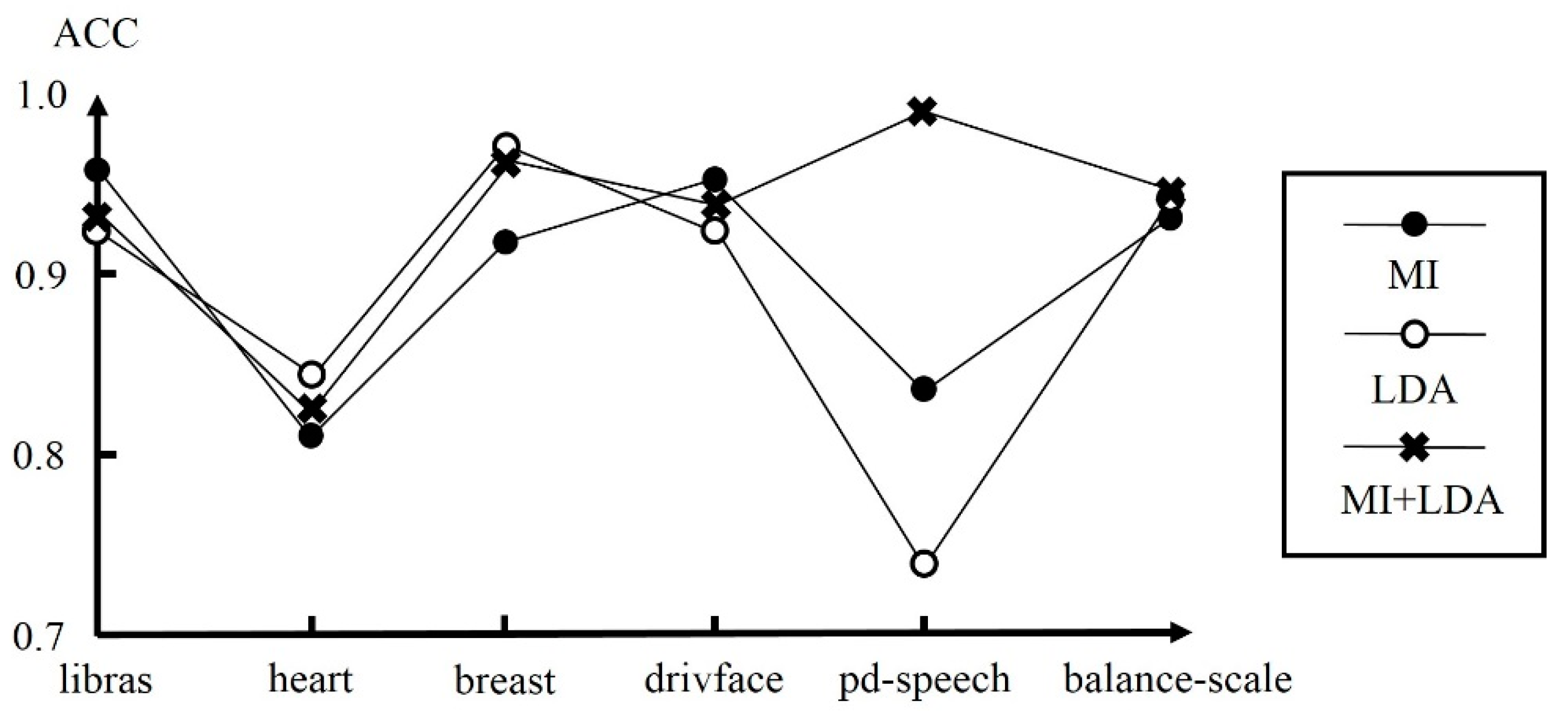
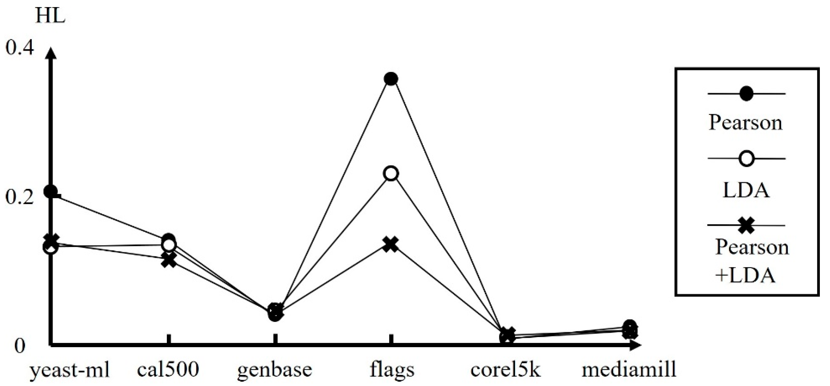
In addition, multiple dimensionality reduction techniques can be used simultaneously to improve performance of RBF networks. Figure 6 shows the performance of SL-Scheme with MI, LDA, and MI+LDA, respectively, for some single-label datasets. As can be seen, MI performs best for the libras and drivface datasets, LDA performs best for the heart and breast datasets, while MI+LDA performs best for the pd-speech and balance-scale datasets. Figure 7 shows the performance of ML-Scheme with Pearson, LDA, and Pearson+LDA, respectively, for some multi-label datasets. As can be seen, Pearson performs best for the yeast-ml, genbase, and mediamill datasets, while Pearson+LDA performs best for the cal500, flags, and corel5K datasets.
4.4. Discussions
The contributions of this work include the determination of the number of neurons in the hidden layer, proposing SL-Scheme and ML-Scheme, respectively, for single-label and multi-label classification, and integrating different techniques to reduce overfitting for multi-class classification. As a result, a classification system can be built more easily due to the simplicity of the schemes and better accuracy can be achieved due to less possibility of overfitting. Also, because of the integration of dimensionality reduction techniques, our proposed schemes can deal with the scalability problem.
There are some RBF implementations available at public websites. One can be accessed from the Weka website, www.cs.waikato.ac.nz/mL/weka. However, this version cannot apply to multi-label multi-class classification. By default, the basis functions are obtained through K-means and the number of hidden nodes is provided by the user. Without integrating with dimensionality reduction techniques, the performance of this implementation is inferior to our SL-Scheme. For example, for the libras dataset, the ACC obtained by the Weka implementation is 0.5861, while SL-Scheme is 0.9641; for the yeast-sl dataset, the ACC obtained by the Weka implementation is 0.8641, while SL-Scheme is 0.9362.
Next, we present some comparisons between RBF and deep learning CNN. The results for single-label datasets obtained by CNN are shown in Table 7. For this table, we ran CNN taken from the MATHWORKS website https://pytorch.org/. Two convolution layers are used, 6 and 12 filters are used in the first and second layers, respectively, the filter size is 3, and ReLU is used as activation function. The car dataset is not used, since all the attributes are discrete, and CNN did not work well. From Table 2 and Table 7, we can see that SL-Scheme performs better in testing accuracy for 11 out of 14 datasets. As mentioned earlier, deep learning networks, e.g., CNN, may have some difficulties. Long training time, due to backpropagation, is required for CNN. For most datasets in Table 7, the training time is tens or even hundreds of seconds long. But for SL-Scheme, the training is done at most in several seconds. The computer used for running the codes is equipped with Intel(R) Core(TM) i7-7700 CPU 3.60 GHz and 16 GB RAM. In a CNN network, the number of hidden layers, the number of kernels, and the kernel size can vary in a wide range. This may lead to a huge search space, and thus finding the best configuration of hyper-parameters from it is a very inefficient and tedious tuning process. Our RBF-based schemes are simpler. The number of layers, i.e., two layers, the Gaussian basis function, the least squares method, and the activation functions associated with the output layer are the decisions taken, while the number of neurons in the hidden layer is the customized parameter and is determined by clustering. Note that the features have been properly selected and designed for the datasets of Table 7. For the datasets without properly extracted features, CNN imposes less burden on the user for feature extraction, compared to traditional classification algorithms. This is a big advantage of deep learning networks. Features can be automatically extracted during the learning phase of the network.
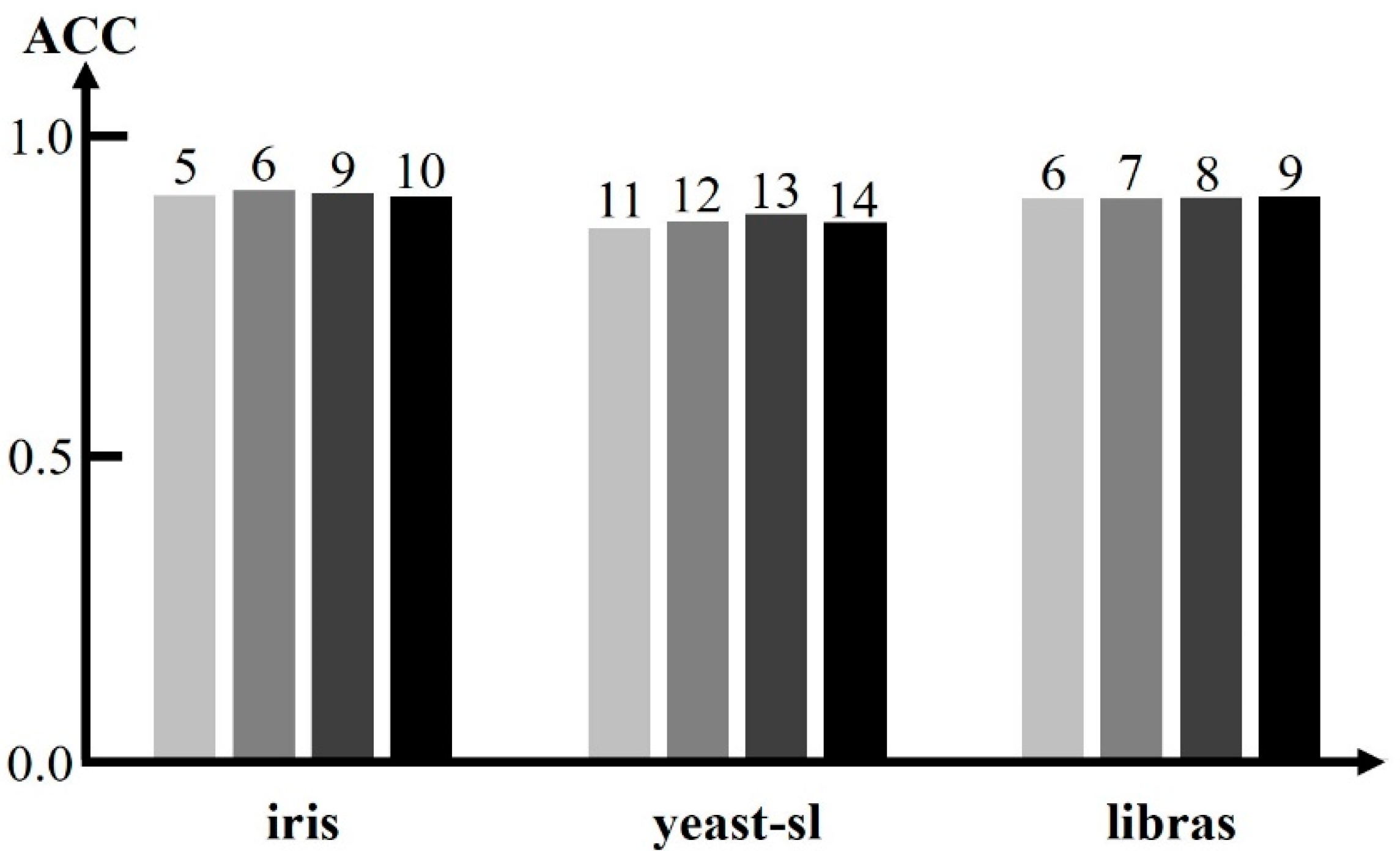
Our schemes are robust. A slight variation in the values of the parameters does not introduce a large variation in performance. Figure 8 shows the ACC of SL-Scheme with variation in the number of hidden neurons in the hidden layer for some datasets. In this figure, three datasets, iris, yeast-sl, and libras, are involved. The number on the top of a bar indicates the number of hidden nodes for the underlying dataset. For example, four cases with the number of hidden nodes being 5, 6, 9, and 10, respectively, are presented for the iris dataset. As can be seen, the ACCs obtained for these four cases do not vary much. Figure 9 shows the ACC of SL-Scheme with variation in the number of input dimensions selected by MI for some datasets. In this figure, three datasets, soybean, ecoli, and libras, are involved. The number on the top of a bar indicates the number of input dimensions selected by MI for the underlying dataset. For example, four cases with the number of input dimensions being 4, 5, 6, and 7, respectively, are presented for the ecoli dataset. The ACCs obtained for these four cases do not vary significantly. Figure 10 shows the ACC of SL-Scheme with variation in the number of input dimensions extracted by LDA for some datasets. In this figure, three datasets, yeast-sl, ecoli, and libra, are involved. The number on the top of a bar indicates the number of input dimensions extracted by LDA for the underlying dataset. For example, four cases with the number of input dimensions being 2, 3, 4, and 5, respectively, are presented for the libras dataset. The ACCs obtained for these four cases are almost identical. Our schemes can deal with a lot of data. For example, ML-Scheme work well with the genbase dataset, which has 1186 attributes and the mediamill dataset, which has 43,907 instances, as shown in Table 4. To show the scalability of SL-Scheme, we ran SL-Scheme on the pen-based dataset which collected samples from writers and has 10,992 instances. A testing accuracy of 0.9841 is obtained.
5. Conclusions and Future Work
We adopt radial basis function (RBF) networks for multi-class classification. RBF networks are two-layer networks with only one hidden layer and can have fewer problems with local minima and learn faster. We have described how the configuration of hyper-parameters is decided and how the curse of dimensionality is reduced for RBF networks. We use an iterative self-constructing clustering to determine the number of hidden neurons. The centers and deviations of the basis functions can also be determined from the clustered results. We have presented several techniques, mutual information, Pearson correlation, information gain, and LDA, to reduce the dimensionality of the inputs to make the RBF networks less likely to overfit.
We have presented two RBF-based neural network schemes for multi-class classification. The first scheme, SL-Scheme, is for single-label multi-class classification. The competitive activation function is used with the output nodes. As a result, an input object can be classified to only one category. The second scheme, ML-Scheme, is for multi-label multi-class classification. The symmetrical hard limit activation function is used with the output nodes. An input object can therefore be classified to two or more categories.
In addition to the techniques adopted, ensemble classification [47,48] can also be applied to deal with the curse of dimensionality problem. An ensemble of classifiers, each of which deals with a small subset of attributes, are created from a given dataset. For an unseen instance, the predicted classifications of the instance for each of the classifiers is computed. By combining the outputs of all the classifiers, the final predicted classifications for the unseen instance is determined. Intuitively, the ensemble of classifiers as a whole can provide a higher level of classification accuracy than any one of the individual classifiers. Overfitting can be improved by reducing the number of hidden nodes in the first layer. Given the basis functions obtained by the SCC clustering algorithm, the orthogonal least squares (OLS) technique [31] can be applied to select the most effective ones. Firstly, the basis function, which creates the largest reduction in error, is selected. Then, one basis function is added at a time until some stopping criterion is met. Furthermore, nested cross validation [49] can be applied to help determine the best configuration of hyperparameters for RBF networks. The total dataset is split in k sets. One by one, a set is selected as the outer test set and the k-1 other sets are combined as the corresponding outer training set. Each outer training set is further sub-divided into sets, and each time a set is selected as the inner test set and the other sets are combined as the corresponding inner training set. For each outer training set, the best values of the hyperparameters are obtained from the inner cross-validation, and the performance of the underlying RBF model is then evaluated using the outer test set. We will investigate these techniques in our future research.
Author Contributions
Individual contributions are: Conceptualization, S.-J.L.; methodology, S.-J.L.; software, Y.-J.Y. and C.-Y.W.; validation, Y.-J.Y., C.-Y.W. and S.-J.L.; formal analysis, S.-J.L.; investigation, S.-J.L. and C.-K.L.; resources, S.-J.L. and C.-K.L.; data curation, Y.-J.Y. and C.-Y.W.; writing—original draft preparation, S.-J.L.; writing—review and editing, S.-J.L. and C.-K.L.; visualization, Y.-J.Y. and C.-Y.W.; supervision, S.-J.L.; project administration, S.-J.L. and C.-K.L.; funding acquisition, S.-J.L. and C.-K.L.
Funding
This research was funded by Ministry of Science and Technology, MOST-106-2321-B-037-003, MOST-107-2221-E-110-065 and MOST-107-2622-E-110-008-CC3, by Environmental Protection Agency, MOST-107-EPA-F-012-001, by NSYSU-KMU Joint Research Project, #NSYSUKMU 108-P042, and by the Intelligent Electronic Commerce Research Center, NSYSU.
Acknowledgments
The anonymous reviewers are highly appreciated for their comments which were very helpful in improving the quality and presentation of the paper.
Conflicts of Interest
The authors declare no conflict of interest.
Appendix A
The iterative self-constructing clustering (SCC) algorithm [32] is an extension of the one proposed in [50]. Let J be the number of existing clusters, initialized to be 0. SCC proceeds iteratively. In the first iteration, for pattern i, (), , the membership degree of pattern i to existing cluster , , is calculated as
If where is a pre-defined constant, it is assumed that pattern is not similar to any existing group. Then, J is increased by 1, i.e., , and a new group is generated, having
where is a pre-defined constant. On the contrary, if and pattern i belongs to the same category of , let cluster be the one with the highest membership degree. Then, pattern i is added to cluster by
When all patterns are processed, SSC stops with J clusters.
In the next iteration, for pattern i, (), , it is removed from the cluster , , to which it was assigned. One of the following three cases occurs:
- If there is no pattern left in , is deleted, and the number of existing clusters is decreased by 1, i.e., .
- If there is only one pattern left in , the characteristics of are reset by Equation (29), taking the left pattern as the single member.
- Otherwise, is updated as
Then, the membership degree of pattern i to , , is calculated by Equation (28), and a new cluster is created by Equation (29) or pattern i is added to an existing cluster by Equations (30)–(32). When all the training patterns are processed, (1) if the cluster assignment of any pattern is changed, the next iteration proceeds; (2) otherwise, the algorithm stops with J clusters together with their centers and deviations.
References
- Duda, R.O.; Hart, P.E.; Stork, D.G. Pattern Classification, 2nd ed.; Wiley & Sons: New York, NY, USA, 2001. [Google Scholar]
- Murty, M.N.; Devi, V.S. Pattern Recognition: An Algorithmic Approach; Springer: Berlin, Germany, 2011. [Google Scholar]
- Lei, Y.; He, Z.; Zi, Y. Application of an intelligent classification method to mechanical fault diagnosis. Expert Syst. Appl. 2009, 36, 9941–9948. [Google Scholar] [CrossRef]
- Rahim, I.M.A.; Mat, F.; Yaacob, S.; Siregar, R.A. The classification of material mechanical properties using non-destructive vibration technique. In Proceedings of the 2011 IEEE 7th International Colloquium on Signal Processing and Its Applications, Penang, Malaysia, 4–6 March 2011. [Google Scholar] [CrossRef]
- Süsstrunk, R.; Huber, S.D. Classification of topological phonons in linear mechanical metamaterials. Proc. Natl. Acad. Sci. USA 2016, 113, E4767–E4775. [Google Scholar] [CrossRef]
- Bhate, D.; Penick, C.A.; Ferry, L.A.; Lee, C. Classification and selection of cellular materials in mechanical design: Engineering and biomimetic approaches. Designs 2019, 3, 19. [Google Scholar] [CrossRef]
- De Vicente, S.M.G.; Prinja, N.; Gagliardi, M.; Rovere, S.L.; Perrault, D.; Taylor, N. Safety classification of mechanical components for fusion application. Fusion Eng. Des. Part B 2018, 136, 1237–1241. [Google Scholar] [CrossRef]
- Ion, J.C. Laser Processing of Engineering Materials: Principles, Procedure and Industrial Application; Elsevier: Amsterdam, The Netherlands, 2012. [Google Scholar]
- Zissis, D. A cloud based architecture capable of perceiving and predicting multiple vessel behaviour. Appl. Soft Comput. 2015, 35, 652–661. [Google Scholar] [CrossRef] [Green Version]
- Zhang, M.-L.; Zhou, Z.-H. A review on multi-label learning algorithms. IEEE Trans. Knowl. Data Eng. 2013, 26, 1819–1837. [Google Scholar] [CrossRef]
- Lee, S.-J.; Jiang, J.-Y. Multi-Label Text Categorization Based on Fuzzy Relevance Clustering. IEEE Trans. Fuzzy Syst. 2014, 22, 1457–1471. [Google Scholar] [CrossRef]
- Fukunaga, K. Introduction to Statistical Pattern Recognition, 2nd ed.; Academic Press: Boston, MA, USA, 1990. [Google Scholar]
- Jain, A.K.; Duin, R.P.W.; Mao, J. Statistical pattern recognition: A review. IEEE Trans. Pattern Anal. Mach. Intell. 2000, 22, 4–37. [Google Scholar] [CrossRef]
- Safavian, S.R.; Landgrebe, D. A survey of decision tree classifier methodology. IEEE Trans. Syst. Man Cybern. 1991, 21, 660–674. [Google Scholar] [CrossRef]
- Bramer, M. Principles of Data Mining, 3rd ed.; Springer: Berlin, Germany, 2016. [Google Scholar]
- Breiman, L. Random forests. Mach. Learn. 2001, 45, 5–32. [Google Scholar] [CrossRef]
- Aha, D.W. Lazy learning: Special issue editorial. Artif. Intell. Rev. 1997, 11, 7–10. [Google Scholar] [CrossRef]
- Zhang, M.-L.; Zhou, Z.-H. ML-KNN: A lazy learning approach to multi-label learning. Pattern Recognit. 2007, 40, 2038–2048. [Google Scholar] [CrossRef] [Green Version]
- Kamiński, B.; Jakubczyk, M.; Szufel, P. A framework for sensitivity analysis of decision trees. Cent. Eur. J. Oper. Res. 2018, 26, 135–159. [Google Scholar] [CrossRef] [PubMed]
- Haykin, S. Neural Networks and Learning Machines, 3rd ed.; Pearson Hall: Upper Saddle River, NJ, USA, 2011. [Google Scholar]
- Ojha, V.K.; Abraham, A.; Snńžel, V. Metaheuristic design of feedforward neural networks: A review of two decades of research. Eng. Appl. Artif. Intell. 2017, 60, 97–116. [Google Scholar] [CrossRef] [Green Version]
- Suykens, J.A.K.; van Gestel, T.; de Brabanter, J.; de Moor, B.; Vandewalle, J. Least Squares Support Vector Machines; World Scientific Publishing Company: Singapore, 2002. [Google Scholar]
- Hsu, C.-W.; Lin, C.-J. comparison of methods for multiclass support vector machines. IEEE Trans. Neural Netw. 2002, 13, 415–425. [Google Scholar] [PubMed]
- Elisseeff, A.; Weston, J. A kernel method for multi-labelled classification. In Advances in Neural Information Processing Systems 14; MIT Press: Cambridge, MA, USA, 2002; pp. 681–687. [Google Scholar]
- Burges, C.J.C. A tutorial on support vector machines for pattern recognition. Data Min. Knowl. Discov. 1998, 2, 121–167. [Google Scholar] [CrossRef]
- LeCun, Y.; Bengio, Y.; Hinton, G. Deep learning. Nature 2015, 521, 436–444. [Google Scholar] [CrossRef] [PubMed]
- Eunsuk, C.; Chulwoo, H.; Parka, F.C. Deep learning networks for stock market analysis and prediction: Methodology, data representations, and case studies. Expert Syst. Appl. 2017, 83, 187–205. [Google Scholar] [Green Version]
- Nabian, M.A.; Meidani, H. Deep Learning for Accelerated Reliability Analysis of Infrastructure Networks. Comput. Aided Civ. Infrastruct. Eng. 2017, 33, 443–458. [Google Scholar] [CrossRef]
- Broomhead, D.S.; Lowe, D. Multivariable function interpolation and adaptive networks. Complex Syst. 1988, 2, 321–355. [Google Scholar]
- Marsupial, D. What Are Alternatives of Gradient Descent? Available online: https://stats.stackexchange.com/q/97026 (accessed on 9 May 2014).
- Hagan, M.T.; Demuth, H.B.; Beale, M.H.; de Jesús, O. Neural Network Design, 2nd ed.; Martin Hagan: Stillwater, OK, USA, 2014. [Google Scholar]
- Wang, Z.-Y. Some Variants of Self-Constructing Clustering; National Sun Yat-Sen University: Kaohsiung, Taiwan, 2017. [Google Scholar]
- Golub, G.H.; van Loan, C.F. Matrix Computations; JHU Press: Baltimore, MD, USA, 2012. [Google Scholar]
- Kraskov, A.; Stgbauer, H.; Grassberger, P. Estimating Mutual Information. Phys. Rev. E 2004, 69, 066138. [Google Scholar] [CrossRef] [PubMed]
- Stojanović, M.B.; Božić, M.M.; Stanković, M.M.; Stavić, Z.P. A methodology for training set instance selection using mutual information in time series prediction. Neurocomputing 2014, 141, 236–245. [Google Scholar] [CrossRef]
- Chen, T.-T.; Lee, S.-J. A weighted LS-SVM learning system for time series forecasting. Inf. Sci. 2015, 299, 99–116. [Google Scholar] [CrossRef]
- Boutell, M.; Luo, J.; Shen, X.; Brown, C. Learning multi-label scene classification. Pattern Recognit. 2004, 37, 1757–1771. [Google Scholar] [CrossRef] [Green Version]
- Chen, W.; Yan, J.; Zhang, B.; Chen, Z.; Yang, Q. Document transformation for multi-label feature selection in text categorization. In Proceedings of the 7th IEEE International Conference on Data Mining, Los Alamitos, CA, USA, 28–31 October 2007; pp. 451–456. [Google Scholar]
- Trohidis, K.; Tsoumakas, G.; Kalliris, G.; Vlahavas, I. Multilabel classification of music into emotions. In Proceedings of the 9th International Conference on Music Information Retrieval (ISMIR 2008), Philadelphia, PA, USA, 14–18 September 2008. [Google Scholar]
- Rodgers, J.L.; Nicewander, W.A. Thirteen ways to look at the correlation coefficient. Am. Stat. 1988, 42, 59–66. [Google Scholar] [CrossRef]
- Li, L.; Wu, J.; Hudda, N.; Sioutas, C.; Fruin, S.A.; Delfino, R.J. Modeling the concentrations of on-road air pollutants in Southern California. Environ. Sci. Technol. 2013, 47, 9291–9299. [Google Scholar] [CrossRef]
- Izenman, A.J. Linear discriminant analysis. In Modern Multivariate Statistical Techniques; Springer: New York, NY, USA, 2013. [Google Scholar]
- Sokolova, M.; Lapalme, G. A systematic analysis of performance measures for classification tasks. Inf. Process. Manag. 2009, 45, 427–437. [Google Scholar] [CrossRef]
- UCI Machine Learning Repository. Available online: https://archive.ics.uci.edu (accessed on 27 July 2019).
- Schneider, P.; Biehl, M.; Hammer, B. Adaptive relevance matrices in learning vector quantization. Neural Comput. 2009, 21, 3532–3561. [Google Scholar] [CrossRef]
- Tsoumakas, G.; Spyromitros-Xioufis, E.; Vilcek, J.; Vlahavas, I. MULAN: A Java library for multi-label learning. J. Mach. Learn. Res. 2011, 12, 2411–2414. [Google Scholar]
- Rieger, S.A.; Muraleedharan, R.; Ramachandran, R.P. Speech based emotion recognition using spectral feature extraction and an ensemble of kNN classifiers. In Proceedings of the 9th International Symposium on Chinese Spoken Language Processing, Singapore, 12–14 September 2014; pp. 589–593. [Google Scholar]
- Gu, Q.; Ding, Y.-S.; Zhang, T.-L. An ensemble classifier based prediction of G-protein-coupled receptor classes in low homology. Neurocomputing 2015, 154, 110–118. [Google Scholar] [CrossRef]
- Wikipedia. Cross-Validation (Statistics). Available online: https://en.wikipedia.org/wiki/Cross-validation_(statistics) (accessed on 27 July 2019).
- Lee, S.-J.; Ouyang, C.-S. A neuro-fuzzy system modeling with selfconstructing rule generation and hybrid SVD-based learning. IEEE Trans. Fuzzy Syst. 2003, 11, 341–353. [Google Scholar]
Figure 1.
Functionality of classification.

Figure 2.
Diagram of single-label (SL)-Scheme for single-label classification.

Figure 3.
Multi-class radial basis function (RBF) network M-RBF.

Figure 4.
Diagram of multi-label (ML)-Scheme for multi-label classification.

Figure 5.
SL-Scheme for the example.

Figure 6.
Performance of SL-Scheme with mutual information (MI), linear discriminant analysis (LDA), and MI+LDA.
Figure 6.
Performance of SL-Scheme with mutual information (MI), linear discriminant analysis (LDA), and MI+LDA.

Figure 7.
Performance of ML-Scheme with Pearson, LDA, and Pearson+LDA.

Figure 8.
Performance of SL-Scheme with variation in the number of hidden neurons.

Figure 9.
Performance of SL-Scheme with variation in the number of input dimensions selected by MI.

Figure 10.
Performance of SL-Scheme with variation in the number of input dimensions extracted by LDA.
Figure 10.
Performance of SL-Scheme with variation in the number of input dimensions extracted by LDA.


Table 1.
Characteristics of the datasets for single-label multi-class classification.
| Dataset | # Attribute | # Instances | # Categories |
|---|---|---|---|
| Iris | 4 | 150 | 3 |
| soybean | 35 | 307 | 4 |
| glass | 10 | 214 | 6 |
| yeast-sl | 8 | 1484 | 10 |
| ecoli | 8 | 336 | 8 |
| car | 6 | 1728 | 4 |
| madelon | 500 | 2600 | 2 |
| wine | 13 | 178 | 3 |
| sonar | 60 | 208 | 2 |
| libras | 91 | 360 | 15 |
| heart | 13 | 270 | 2 |
| breast | 30 | 569 | 2 |
| drivface | 6400 | 606 | 3 |
| pd-speech | 26 | 1040 | 2 |
| balance-scale | 5 | 625 | 3 |
Table 2.
Testing accuracy (ACC) obtained by different methods.
| Dataset | SVM | DT | KNN | MLP | LVQ | RandForest | SL-Scheme |
|---|---|---|---|---|---|---|---|
| Iris | 0.9660 | 0.9600 | 0.9689 | 0.9822 | 0.9933 | 0.9511 | 0.9788 |
| soybean | 1 | 1 | 0.9894 | 0.9400 | 1 | 0.9389 | 0.9889 |
| glass | 0.9070 | 0.9065 | 0.9081 | 0.9423 | 0.6733 | 0.9922 | 0.9783 |
| yeast-sl | 0.9185 | 0.9098 | 0.9197 | 0.9055 | 0.3187 | 0.9156 | 0.9362 |
| ecoli | 0.8720 | 0.9509 | 0.9635 | 0.8366 | 0.8930 | 0.8285 | 0.9661 |
| car | 0.9818 | 0.9777 | 0.9864 | 0.9737 | 0.9770 | 0.9792 | 0.9656 |
| madelon | 0.6746 | 0.7223 | 0.6646 | 0.5035 | 0.6639 | 0.7227 | 0.7546 |
| wine | 0.9888 | 0.9476 | 0.9813 | 0.5694 | 0.7868 | 0.9517 | 0.9924 |
| sonar | 0.8413 | 0.7548 | 0.8029 | 0.8271 | 0.8799 | 0.7264 | 0.9031 |
| libras | 0.9804 | 0.9507 | 0.9811 | 0.9596 | 0.7028 | 0.9719 | 0.9641 |
| heart | 0.8407 | 0.7704 | 0.8333 | 0.7556 | 0.8704 | 0.7481 | 0.8593 |
| breast | 0.9772 | 0.9051 | 0.9631 | 0.5182 | 0.9261 | 0.9157 | 0.9789 |
| drivface | 0.9692 | 0.9560 | 0.9692 | 0.9582 | 0.9587 | 0.9648 | 1.0000 |
| pd-speech | 0.8532 | 0.7870 | 0.9061 | 0.7434 | 0.8577 | 0.8095 | 0.9987 |
| balance-scale | 0.9445 | 0.8507 | 0.8592 | 0.9776 | 0.9267 | 0.8645 | 0.9413 |
| average | 0.9413 | 0.8900 | 0.9131 | 0.8262 | 0.8288 | 0.8854 | 0.9453 |
Table 3.
Characteristics of the datasets for multi-label multi-class classification.
| Dataset | # Attribute | # Instances | # Categories | Cardinality |
|---|---|---|---|---|
| birds | 260 | 645 | 19 | 1.014 |
| scene | 294 | 2407 | 6 | 1.074 |
| emotions | 72 | 593 | 6 | 1.869 |
| yeast-ml | 103 | 2417 | 14 | 4.237 |
| cal500 | 68 | 502 | 174 | 26.044 |
| genbase | 1186 | 662 | 27 | 1.252 |
| flags | 19 | 194 | 7 | 3.392 |
| corel5k | 499 | 5000 | 374 | 3.522 |
| mediamill | 120 | 43,907 | 101 | 4.376 |
Table 4.
Testing Hamming Loss (HL) obtained by different methods.
| Dataset | ML-SVM | DT | ML-KNN | MLP | LVQ | RandForest | ML-Scheme |
|---|---|---|---|---|---|---|---|
| birds | 0.1154 | 0.2237 | 0.0510 | 0.2496 | 0.2259 | 0.2291 | 0.0460 |
| scene | 0.1568 | 0.2094 | 0.1130 | 0.2933 | 0.2325 | 0.1994 | 0.0602 |
| emotions | 0.2343 | 0.2428 | 0.2302 | 0.2967 | 0.1652 | 0.2192 | 0.1497 |
| yeast-ml | 0.2108 | 0.2787 | 0.2136 | 0.3122 | 0.1059 | 0.3130 | 0.1429 |
| cal500 | 0.1380 | 0.2137 | 0.1400 | 0.1679 | 0.2286 | 0.1567 | 0.1263 |
| genbase | 0.0015 | 0.0302 | 0.0020 | 0.1366 | 0.1765 | 0.1194 | 0.0016 |
| flags | 0.2791 | 0.213 | 0.3099 | 0.2636 | 0.1493 | 0.2497 | 0.1466 |
| corel5k | 0.0090 | 0.0720 | 0.0654 | 0.0968 | 0.1160 | 0.0406 | 0.0088 |
| mediamill | 0.0335 | 0.1158 | 0.1024 | 0.1567 | 0.1752 | 0.1267 | 0.0204 |
| average | 0.1309 | 0.1775 | 0.1364 | 0.2193 | 0.1750 | 0.1838 | 0.0781 |
Table 5.
Testing ACC obtained by SL-Scheme with different reduction techniques.
| Dataset | WO | MI | Pearson | LDA | IG |
|---|---|---|---|---|---|
| iris | 0.9689 | 0.9689 | 0.9689 | 0.9778 | 0.9689 |
| soybean | 0.9778 | 0.9778 | 0.8727 | 0.6808 | 0.9889 |
| yeast-sl | 0.9362 | 0.8966 | 0.8924 | 0.8976 | 0.8880 |
| ecoli | 0.7806 | 0.9661 | 0.8765 | 0.9329 | 0.9433 |
| wine | 0.9555 | 0.9367 | 0.7461 | 0.9924 | 0.9364 |
| libras | 0.9548 | 0.9641 | 0.9300 | 0.9300 | 0.9585 |
| breast | 0.9318 | 0.9298 | 0.6241 | 0.9789 | 0.9213 |
| average | 0.9294 | 0.9486 | 0.8444 | 0.9129 | 0.9436 |
Table 6.
Testing HL obtained by ML-Scheme with different reduction techniques.
| Dataset | WO | MI | Pearson | LDA | IG |
|---|---|---|---|---|---|
| birds | 0.0466 | 0.0687 | 0.0546 | 0.1065 | 0.0460 |
| emotion | 0.3966 | 0.3751 | 0.2874 | 0.1497 | 0.3793 |
| yeast-ml | 0.2131 | 0.2144 | 0.1429 | 0.2071 | 0.2079 |
| genbase | 0.0016 | 0.0345 | 0.0421 | 0.0452 | 0.0018 |
| mediamill | 0.0299 | 0.0284 | 0.0204 | 0.0322 | 0.0300 |
| average | 0.1376 | 0.1442 | 0.1095 | 0.1081 | 0.1330 |
Table 7.
Results for single-label datasets obtained by CNN.
| Dataset | ACC | Time(s) | Dataset | ACC | Time(s) |
|---|---|---|---|---|---|
| iris | 0.9667 | 7.0531 | soybean | 1.0000 | 3.4581 |
| glass | 0.6744 | 10.6245 | yeast-sl | 0.6027 | 66.0174 |
| ecoli | 0.8088 | 16.3213 | madelon | 0.5135 | 248.2281 |
| wine | 0.9722 | 9.1674 | sonar | 0.9286 | 12.2143 |
| libras | 0.9028 | 21.5882 | heart | 0.8197 | 14.5280 |
| breast | 0.9649 | 29.1769 | drivface | 0.9754 | 405.3066 |
| pd-speech | 0.8421 | 107.1434 | balance-scale | 0.9600 | 28.4199 |
© 2019 by the authors. Licensee MDPI, Basel, Switzerland. This article is an open access article distributed under the terms and conditions of the Creative Commons Attribution (CC BY) license (http://creativecommons.org/licenses/by/4.0/).
Share and Cite
MDPI and ACS Style
You, Y.-J.; Wu, C.-Y.; Lee, S.-J.; Liu, C.-K. Intelligent Neural Network Schemes for Multi-Class Classification. Appl. Sci. 2019, 9, 4036. https://doi.org/10.3390/app9194036
AMA Style
You Y-J, Wu C-Y, Lee S-J, Liu C-K. Intelligent Neural Network Schemes for Multi-Class Classification. Applied Sciences. 2019; 9(19):4036. https://doi.org/10.3390/app9194036
Chicago/Turabian StyleYou, Ying-Jie, Chen-Yu Wu, Shie-Jue Lee, and Ching-Kuan Liu. 2019. "Intelligent Neural Network Schemes for Multi-Class Classification" Applied Sciences 9, no. 19: 4036. https://doi.org/10.3390/app9194036
Note that from the first issue of 2016, this journal uses article numbers instead of page numbers. See further details here.