Abstract
Purpose: Localization and mapping with LiDAR data is a fundamental building block for autonomous vehicles. Though LiDAR point clouds can often encode the scene depth more accurate and steadier compared with visual information, laser-based Simultaneous Localization And Mapping (SLAM) remains challenging as the data is usually sparse, density variable and less discriminative. The purpose of this paper is to propose an accurate and reliable laser-based SLAM solution. Design/methodology/approach: The method starts with constructing voxel grids based on the 3D input point cloud. These voxels are then classified into three types to indicate different physical objects according to the spatial distribution of the points contained in each voxel. During the mapping process, a global environment model with Partition of Unity (POU) implicit surface is maintained and the voxels are merged into the model from stage to stage, which is implemented by Levenberg–Marquardt algorithm. Findings: We propose a laser-based SLAM method. The method uses POU implicit surface representation to build the model and is evaluated on the KITTI odometry benchmark without loop closure. Our method achieves around 30% translational estimation precision improvement with acceptable sacrifice of efficiency compared to LOAM. Overall, our method uses a more complex and accurate surface representation than LOAM to increase the mapping accuracy at the expense of computational efficiency. Experimental results indicate that the method achieves accuracy comparable to the state-of-the-art methods. Originality/value: We propose a novel, low-drift SLAM method that falls into a scan-to-model matching paradigm. The method, which operates on point clouds obtained from Velodyne HDL64, is of value to researchers developing SLAM systems for autonomous vehicles.
1. Introduction
Reliable localization of autonomous vehicles is an attractive research topic since it is a basic requirement for navigation and other tasks [1,2,3,4,5]. Fully autonomous vehicles should reliably locate themselves, ideally by using only their own sensors on board without relying on external information sources such as GPS. In scenarios where such external information is absolutely unavailable, Simultaneous Localization And Mapping (SLAM) is always an alternative option.
SLAM has been intensively studied in the past few decades and various solutions based on different sensors have been proposed for both indoor and outdoor environments. In outdoor scenes, the advantage of LiDAR with respect to cameras is that the noise associated with each measurement is independent of the distance itself and usually more robust to the illumination variation. Therefore, laser-based SLAM is becoming one of the mainstream solutions in outdoor scenes. Most laser-based SLAM methods tend to extract stable features such as planes and edges from points, and then do SLAM in a ‘feature space’. They are therefore categorized as feature-based SLAM, whose performance is mainly determined by two factors. The first factor is the way features are designed. Ji Zhang et al. [6,7] propose a planar and edge feature designing method based on curvature. Michael Bosse et al. [8] incorporate shape information which is calculated from geometric statistics of the point cloud into the Iterative Closest Point (ICP) correspondence step. The second factor is the scan matching method. Scan-to-scan and scan-to-model matching are the two main scan matching frameworks in SLAM. Sen Wang et al. [9] propose a scan-to-scan odometry trajectory estimation method by using convolutional neural networks to process LiDAR point clouds. KinectFusion [10] implements scan-to-model matching by using an implicit surface as model. The state-of-the-art laser-based SLAM method, LiDAR Odometry And Mapping (LOAM) [6] extracts distinct features corresponding to physical surfaces and corners. To enable on-line implementation, LOAM switches between scan-to-scan at 10 Hz and scan-to-model operation at 1 Hz update frequency. Although LOAM has achieved good performance, there are still challenges in outdoor applications using 3D laser sensors, i.e., (1) inherent point matching error since the sparsity of the point clouds, which means that there are always existing errors when we directly use the sparse point cloud to fit the surface of environment. Furthermore, it is nearly impossible to obtain rigid point correspondences between scans; (2) it is hard to fix the matching parameter since the density variation of the point clouds. During the feature-based matching process, it is required to extract enough context information of one 3D point to make it discriminative, while the scope of the dominating context is greatly affected by the point density. In this paper, to tackle the above challenges, we introduce POU implicit surface representation to regress the environment surface with sparsity points, which can effectively encode the detailed geometrical information. We discretize the point cloud into 3D voxels. These voxels are classified into planar and edge feature voxels according to the geometrical character of the points contained in the voxel. Finally, we build a feature voxel map for further scan-to-model matching, during which the POU implicit surface representation is proposed to adapt to the voxel map. The key contributions of our work are as follows:
- (1)
- We propose a novel feature voxel map which stores voxels with salient planar or edge features.
- (2)
- We propose a scan-to-model matching framework using POU implicit surface representation.
The rest of this paper is organized as follows. In Section 2, we discuss related work and conclude how our work is different from the state of the art. The feature extraction Algorithm 1 is presented with details in Section 3, and the scan-to-model matching Algorithm 1 is given in Section 4. Experimental results are shown in Section 5. Finally, Section 6 concludes the paper.
2. Related Work
SLAM with cameras and LiDAR has attracted wide attention both from robotic and computer vision communities. We acknowledge the large body of work in this field, but concentrate here only on approaches based on LiDAR. Since feature extraction, laser-based mapping and scan-matching framework are the three most important steps for laser-based SLAM, we therefore look into related work on these three aspects and provide general ideas on how they work as following.
Feature extraction: LOAM focuses on edge and planar features in the LiDAR sweep and keep them in a map for edge-line and plane-planar surface matching. Tixiao Shan et al. [11] also use edges and planar features to solve different components of the 6-DOF transformation across consecutive scans. While these works extract features based on curvature, there is still difference, as the method by [11], which is ground-optimized, as it leverages the presence of a ground plane in its segmentation and optimization steps. Using point cloud obtained from a high resolution and high density Zoller–Fröhlich Z+F laser, J Lalonde and Yungeun Choe et al. [12,13] exploit point cloud geometrical statistics to classify the natural terrain into scatter-ness, linearity, and surface-ness. Using point cloud from a SICK LMS291 laser range sensor, Michael Bosse et al. [8] implement scan-matching based on point cloud geometrical statistics features. They use ICP to align voxel centroids, which can reduce the number of points for scan matching as well as the size of the map. In contrast to [8], we consider the geometric features of the points more subtly and implement scan matching with original points, which would not lead to information loss.
Laser-based mapping: SLAM systems often build and maintain environment maps, such as the feature map [6,7,11,14,15], dense map [16,17], subsampled clouds [18,19] and Normal Distributions Transform (NDT)-based map [20,21]. In laser-based SLAM systems, the feature map is usually a structural collection of surfaces and corners that are extracted from original point clouds. In this paper, we build a feature map, which can be distinguished from methods in the literature in the way that we maintain more types of features in the form of voxels.
Scan matching framework: Recently, some laser-based SLAM systems use scan-to-model matching framework and achieved state-of-the-art performance using the KITTI odometry benchmark. Jens Behley et al. [16] propose a dense approach to laser-based SLAM that operates on point clouds obtained from Velodyne HDL-64. They construct a surfel-based map and use a point-to-plane ICP [22,23] to estimate the pose transformation of the vehicle. Our method essentially belongs to scan-to-model matching framework. The distinction is that we build a feature voxel map and use POU implicit surface representation to adapt to the scan-to-model matching process based on feature voxel map.
Partition of unity approach: The POU approach has been widely used in surface reconstruction. Ireneusz Tobor et al. [24] show how to reconstruct multi-scale implicit surfaces with attributes, given discrete point sets with attributes. Tung-Ying Lee et al. [25] propose a new 3D non-rigid registration algorithm to register two multi-level partition of unity implicit surfaces with a variational formulation.
3. Feature Extraction
Similar to [26], the scan-to-model matching is triggered when there are salient geometrical features in local regions. So, it is important to find these regions first. In contrast to 3D object classification [27,28] and place recognition [29,30], which use complex point cloud descriptor to segment and classify objects, we use a simpler shape parameterization because our task focuses on incremental transformation for which we have a stronger prior on the relative poses.
3.1. Computing Shape Parameters
A local region that is occupied by the input point cloud is repeated divided until the number of points fall into each voxel is equal to the threshold . The threshold is related to the horizontal and vertical resolution of LiDAR point cloud. In the process of feature extracting, the densities of features in corresponding voxels vary. We consider the density while searching for the correspondences of the features. The lower the density of the features, the lower the probability of finding enough correspondences within a certain radius is. Our experiment results are achieved when is set to 25. Each voxel contains points that fall into it and voxel centroid. The points that fall into voxel are defined as . The first and second-order moments describe the parameters for spatial distribution of the points :
Inspired by [8], the matrix S is decomposed into principal components ordered by increasing eigenvalues. are eigenvectors corresponding to the eigenvalues respectively, where . In the case that the structure of points in a voxel is a linear structure, the principal direction will be the tangent at the curve, with . In the case that the structure of points in a voxel is a solid surface, the principal direction is aligned with the surface normal with . The two saliency features, named linear feature and surface feature, are linear combinations of the eigenvalues. Figure 1 illustrates the two features used. The quantity:
is the linear feature of the points in voxel which ranges from 0 to 1. Similarly the quantity:
is the surface feature of the points in voxel which ranges from 0 to 0.5.
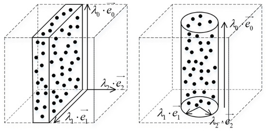
Figure 1.
Illustration of the surface feature and linear feature.
3.2. Voxel Sampling Strategy
Essentially, the voxel-based scan matching process is to construct the associations between voxels. It is believed that voxels with high quantity of linearity or planarity tend to be more stable than others. So for each input point cloud, we classify its 3d grids according to the proposed quantities into three types: edge voxel, planar voxel and others. Furthermore, it should be noticed that the ground points usually contain more planar features and non-ground points usually contain both planar and edge features. With these born in mind, we first divide the whole point cloud into ground and non-ground segments using the method proposed in [31]. Figure 2a is an example of the ground segmentation result. Then, for the non-ground points, we extract planar and edge features, while only planar features are extracted for the ground points.
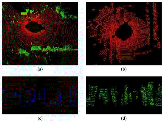
Figure 2.
(a) is the result of ground segmentation. In (a), the red points are labeled as ground points and the green points are labeled as non-ground points. (b–d) are the ground planar features, non-ground edge features and non-ground planar features.
In each scan, which is now represented as the voxel centroids, we sort the voxels based on their linearity values c and surface-ness values p and get two sorted lists. Two thresholds and are then employed to distinguish different types of features. We call the voxels with c larger than edge features, and the voxels with p larger than planar features. Then edge features with the maximum c are selected from each scan. Non-ground and ground planar features with the maximum p are also selected, and the numbers of the two types of features are and , respectively. Edge and planar features extracted from all the scans are denoted as , and thereafter. Visualization examples of these features are given in Figure 2b–d.
4. Scan-To-Model Matching with POU Implicit Surface Representation
Once the currant laser scan is transformed into a set of stable voxels, we implement scan-to-model matching process. In our method, the map consists of the last n located feature sets , and . Let
be the map that contains planar features and edge features at time k. To better fit the observed surface with these points and adapt to the feature voxel map, we take the POU implicit surface representation to construct the model.
4.1. Finding Feature Point Correspondence
In the current scan, each point is labeled according to the type of its corresponding voxel. During the matching process, we construct the correspondences between voxels in the map and the current feature points with the guidance of labels and Euclidean distance. Since such correspondences generating mechanism narrows down the potential candidates for correspondences, it can help to improve the matching accuracy and efficiency. The detailed correspondence construction process is given below.
For each current edge point in feature set , we search for voxels of
inside a sphere space whose radius is . For each corresponding voxel, we find an edge line as the correspondence of the current edge point. After finding all the correspondence edge lines, we can get the projection points of the current edge point on the corresponded edge lines. Then we use linear quantity c to determine whether can be represented as an edge line. If can be represented as an edge line, it is then regarded as the correspondence of the current edge point. After the edge feature correspondences are obtained, we compute the distance from an edge feature point to its correspondence. The procedure of finding an edge line and the distance computation can be found in [6].
For each current planar point in feature sets and , we respectively find and voxels of
and
inside a sphere space whose radius is as the corresponding voxels. Then, we use the corresponding voxels to construct the POU implicit surface representation of the model, and compute the distance from a planar feature point to its implicit surface representation of the model. The details of building the POU implicit surface representation and computing the distance from a planar feature point to its implicit surface representation of the model will be discussed below.
4.2. POU Implicit Surface Representation for Planar Features
4.2.1. POU Approach
The basic idea of the POU approach is to break the data domain into several pieces, approximate the data in each subdomain separately, and then blend the local solutions together using smooth, local weights that sum up to one everywhere in the domain. More specifically, we assign a specific planar patch as the correspondence of a planar feature point in each correspondence voxel. The procedure of finding the specific points to form planar patches can be found in [7]. We can calculate distances d between the planar feature point and the corresponding planar patches . Then, we project planar feature point x on the surface of planar patches defined by : , where is the normal of the closest point to x in each planar patch and is a good approximation of the surface normal at the projected point . Each planar patch can be regarded as a subdomain. Then, we use the weight function to blend the subdomains together.
4.2.2. POU Implicit Surface Representation
The implicit surface is defined as the set of zeros of a function , which also behaves as a distance function from x to the implicit surface. In this work, we use the POU implicit surface representation.
Similar to the POU implicit surface framework in [32], we define the POU implicit function as an approximate distance of planar feature point at time k to the POU implicit surface defined by the map :
where is the projected points on the corresponding planar patch , is the normal at point . For approximation, we use the quadratic B-spline to generate weight functions for planar patches.
where is the geometric center of planar patch and is a spherical support radius of the planar patch . The function is proportional to the distance between x and and inversely proportional to . It means that the closer to the x, the higher weight will be allocated. And the more scattered the points that form the planar patch are, the higher the weight. In addition to computing the distance from the feature point to the model surface, the surface normal at the projected point of the feature point x should also be computed. In this work, we use the normal of the closest point to x as the approximation of the surface normal at the projected point. Compared with the method using only one plane to represent a surface (could be cylinder or sphere, etc.), we adopt multiple local planes with various planarities to represent a surface which can achieve higher accuracy and obtain more accurate distances from feature points to their correspondences. Figure 3 shows the illustration of POU implicit surface.
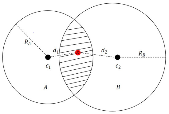
Figure 3.
Illustration of POU implicit surface. Two cells, A and B, are associated with their support radius and , respectively. The value of a point x in the slashed region can be evaluated by ; ; , where and are the distances from the point x to the and , respectively, and are the support radius, and are local plane functions.
4.2.3. Motion Estimation
With distances from feature points to their correspondences in hand, we assign a bisquare weight [7] for each feature point. The rules are twofold. In general, when the distance between the feature point and its correspondence is below a certain threshold, the weight is assigned inversely proportional to the distance. However, when the distance is greater than the threshold, the feature point is regarded as an outlier. We proceed to recover the LiDAR motion by minimizing the overall distances.
First, the following equation is used to project feature point x to the map, namely ,
in which, R and are the rotation matrix and translation vector corresponding to the pose transform T between current scan and the map. By combining the distances and weights from feature points to their correspondences and Equation (11), we derive a geometric relationship between feature points and the corresponding model,
where each row of f corresponds to a feature point, and d contains the corresponding distances. Finally, we obtain the LiDAR motion with the Levenberg–Marquardt method [33]. We do scan matching between the current scan with the last n scans, and the final result is obtained by aggregating the successfully matched scans. Literally, by matching the current scan with the historical n scans, the error propagation problem can be suppressed. As for blunder, we limit the scale of the relative transformation between the current scan and the model. When the blunder occurs, we will abandon the result of the current scan and subsequent scan-matching implementation would be slightly affected. After computing the transformation between the scan and model, we add feature voxels corresponding to current scan to the map and remove the feature voxels corresponding to the oldest scan to always keep n scans for scan matching.
| Algorithm 1: POU-SLAM Scan To Model Matching Framework |
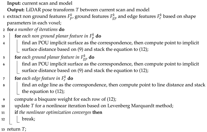 |
5. Experimental Evaluation
5.1. Tests on the Public Dataset KITTI
We evaluate our method using the KITTI odometry benchmark [34], where we use point clouds from a vertical Velodyne HDL-64E S2 mounted on the roof of a car, with a recording rate of 10 Hz. The dataset is composed of a wide variety of environments (urban city, rural road, highways, roads with a lot of vegetation, low or high traffic, etc.). The LiDAR measurements are de-skewed with an external odometry, so we do not apply ego-motion algorithm to this dataset. Table 1 shows the results of our method for all sequences in detail. The relative error is evaluated by the development kit provided with the KITTI benchmark. The data sequences are split into subsequences of 100, 200, …, 800 frames. The error of each subsequence is computed as:
where is the expected position (from ground truth) and is the estimated position of the LiDAR where the last frame of subsequence was taken with respect to the initial position (within given subsequence). The difference is divided by the length of the followed trajectory. The final error value is the average of errors across all the subsequences of all the lengths.

Table 1.
Results On KITTI Odometry.
We include here for comparison the reported results of LOAM, a laser-based odometry approach that switches between scan-to-scan and scan-to-model framework, and the reported results of SUMA [16] a laser-based odometry approach using scan-to-model framework. We can see that the proposed method yields results generally on par with the state-of-the-art in laser-based odometry and often achieves better results in terms of translational error. Overall, we achieve an average translational error of 0.61% compared to 0.84% translsational error of LOAM on KITTI odometry benchmark. We can see that the proposed method yields results generally on par with the state-of-the-art in laser-based odometry and often achieves better results in terms of translational error. Figure 4 shows the sample results using the KITTI benchmark datasets.
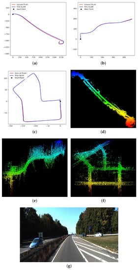
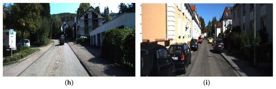
Figure 4.
Sample results using the KITTI benchmark datasets. The datasets are chosen from three types of environments: highway, country and urban from left to right, corresponding to sequences 01, 03, and 07. In (a–c), we compare estimated trajectories of the vehicle to the GPS/INS ground truth. The mapping results are shown in (d–f). An image is shown from each dataset to illustrate the environment, in (g–i).
5.2. Discussion of the Parameter and Performance
In our experiment, we define the thresholds and based on the KITTI Odometry sequence 01. Laser scans contained in this dataset are collected from a highway, the scenario where there is only a very few distinct structural features could be used for scan matching. To extract as many as possible features to accomplish the SLAM task, the thresholds should be set to a fairly low level. It is because the smaller the thresholds, features on spheres or cylinders are more likely to be extracted. These sphere and cylinder features themselves are not planar, and if represented by planes directly can bring about errors that would further reduce the accuracy of the downstream algorithms. In this paper, we blend each planar patch extracted with the weighted function under the implicit surface representation mechanism. This explains why we achieve obvious improvement on this sequence. Therefore, if the thresholds can perform well on such structural feature lacking scenarios, they should be easily transferred to and work in scenarios with richer structural features. For more structured environment such as urban case, the thresholds can be further increased to compromise between the feature richness and the planarity, which promises an accuracy improvement to the whole SLAM algorithm. Table 2 shows the influence of to the result. When is set too large, we can not extract enough features and the result gets worse. Table 3 shows the influence of for ground features to the result. The quantity c as shown in (3) of ground features is generally large and the threshold has a slight influence on the result. Figure 5 shows the variation of the number of non-ground features in different frames on sequence 01 when is set to 0.85. The average number of non-ground features is about 7200. Deschaud [35] holds the view that the pose estimation result is related to the number and distribution of features. The features of different position contribute to different angles and translations. They sample 1000 features based on their sampling strategy which considers the feature distribution and achieve great result. Compared with their method, we do not use a sampling strategy but use more features which compensate for the influence of feature distribution on the results to a certain extent. In our method, the variance of the feature numbers has an influence on the extracted feature distributions and thus further influences the performance. However, since we extract enough number of features for scan-matching, which is more than 2000 at least, there is little influence on the translational error when the number of features drops.
Table 2.
The Influence of for Non Ground Features to the Result.
Table 3.
The Influence of for Ground Features to the Result.
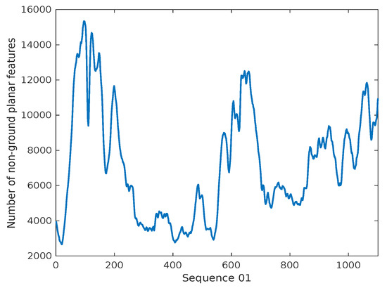
Figure 5.
Variation of the number of non-ground planar features in different frames on sequence 01.
The parameter n is set to 40 for the KITTI odometry benchmark. Table 4 shows the the influence of parameter n. Parameters , and are set to 3 for the KITTI odometry benchmark. In Table 5, we implement camparison experiments in which all the weights of planar patches are the same. We can tell that the performance is significantly improved due to the application of POU framework and the result reaches the best when is set to 3. When is set too large, the correspondences are far away from the current scan features and do not contribute to local surface reconstruction.
Table 4.
Importance of the Parameter n.
Table 5.
Comparison of drift KITTI training dataset between POU Weight and the Same Weight.
5.3. Discussion of the Processing Time
The operating platform in our experiment is Intel i7-7820@3.60 GHz with 16 GB RAM. Our method is evaluated by processing KTTI datasets rather than being deployed in an autonomous vehicle. With regarding to real time implementation, which heavily depends on the hardware configuration, we cannot assert if our method is real time or not. However, we can still provide some of the parameters so people can know the runtime performance of our method. First, we split the point cloud into voxels which contain certain numbers of points and calculate the linear-ness values and surface-ness value for these voxels. It takes 0.5 s. Second, we do scan matching for each feature. The time cost depends on the number of features. For KITTI Odometry sequence 01, the runtime is about 1.5 s. Taking both the above factors into consideration, our SLAM runs at 2 s per scan with one thread. For comparison, LOAM runs at 1 s per scan on the same KITTI dataset. The reason is that compared to LOAM which extract two-dimensional curvature features, we construct voxel grids and extract features according to the spatial distribution of the points contained in each voxel. This results in better accuracy (refer to Table 1) with a slight sacrifice of efficiency.
6. Conclusions
We present a new 3D LiDAR SLAM method that is composed of a new feature voxel map and a new scan-to-model matching framework. We build a novel feature voxel map with voxels including salient shape characteristics. In order to adapt to the proposed map, we implement scan-to-model matching using POU implicit surface representation to blend the correspondence voxels in map together. Our method achieves an average translational error of 0.61% compared to 0.84% translational error of LOAM on KITTI odometry benchmark. The mapping accuracy is improved due to the application of the POU surface model. However, to implement feature matching based on the POU model burdens our system with more computation cost. Our method runs at 2 s per scan with one thread. For comparison, LOAM runs at 1 s per scan on the same KITTI dataset under the scan to model matching framework. As is shown in the the experimental results, the proposed method yields accurate results that are on par with the state-of-the-art. Future work will proceed in two directions. From the research perspective, a specific and efficient octree will be designed to get a 3D grid. Meanwhile, we will deploy the method to fulfill real time application with the aid of multiple threads or GPU to accelerate data processing.
Author Contributions
J.J., J.W. and P.W. developed the method, carried out the experiments and wrote the manuscript. Z.C. gave the research direction and ideas, and put forward amendments and improvements to the manuscript.
Funding
This research was funded by the National Natural Science Fund of China grant number 91848111, 61703387.
Acknowledgments
This work is supported by the National Natural Science Fund of China (Grant No. 91848111, 61703387).
Conflicts of Interest
The authors declare no conflict of interest.
References
- Wang, J.; Chen, Z. A novel hybrid map based global path planning method. In Proceedings of the 2018 3rd Asia-Pacific Conference on Intelligent Robot Systems (ACIRS), Singapore, 21–23 July 2018; pp. 66–70. [Google Scholar]
- Wang, J.; Wang, P.; Chen, Z. A novel qualitative motion model based probabilistic indoor global localization method. Inf. Sci. 2018, 429, 284–295. [Google Scholar] [CrossRef]
- Wang, P.; Zhang, Q.-B.; Chen, Z.-H. A grey probability measure set based mobile robot position estimation algorithm. Int. J. Control Autom. Syst. 2015, 13, 978–985. [Google Scholar] [CrossRef]
- Zhang, Q.; Wang, P.; Chen, Z. Mobile robot pose estimation by qualitative scan matching with 2d range scans. J. Intell. Fuzzy Syst. 2019, 36, 3235–3247. [Google Scholar] [CrossRef]
- Xiong, H.; Chen, Y.; Li, X.; Chen, B.; Zhang, J. A scan matching simultaneous localization and mapping algorithm based on particle filter. Ind. Robot Int. J. 2016, 43, 607–616. [Google Scholar] [CrossRef]
- Zhang, J.; Singh, S. Loam: Lidar odometry and mapping in real-time. In Proceedings of the Robotics: Science and Systems X, Berkeley, CA, USA, 12–16 July 2014. [Google Scholar]
- Zhang, J.; Singh, S. Low-drift and real-time lidar odometry and mapping. Auton. Robots 2017, 41, 401–416. [Google Scholar] [CrossRef]
- Bosse, M.; Zlot, R. Continuous 3d scan-matching with a spinning 2d laser. In Proceedings of the 2009 IEEE International Conference on Robotics and Automation, Kobe, Japan, 12–17 May 2009; pp. 4244–4251. [Google Scholar]
- Wang, S.; Clark, R.; Wen, H.; Trigoni, N. Deepvo: Towards end-to-end visual odometry with deep recurrent convolutional neural networks. In Proceedings of the 2017 IEEE International Conference on Robotics and Automation (ICRA), Singapore, 29 May–3 June 2017; pp. 2043–2050. [Google Scholar]
- Newcombe, R.A.; Izadi, S.; Hilliges, O.; Molyneaux, D.; Kim, D.; Davison, A.J.; Kohi, P.; Shotton, J.; Hodges, S.; Fitzgibbon, A. Kinectfusion: Real-time dense surface mapping and tracking. In Proceedings of the 2011 10th IEEE International Symposium on Mixed and Augmented Reality, Basel, Switzerland, 26–29 October 2011; pp. 127–136. [Google Scholar]
- Shan, T.; Englot, B.J. Lego-loam: Lightweight and ground-optimized lidar odometry and mapping on variable terrain. In Proceedings of the 2018 IEEE/RSJ International Conference on Intelligent Robots and Systems (IROS), Madrid, Spain, 1–5 October 2018; pp. 4758–4765. [Google Scholar]
- Lalonde, J.-F.; Vandapel, N.; Huber, D.F.; Hebert, M. Natural terrain classification using three-dimensional ladar data for ground robot mobility. J. Field Robot. 2006, 23, 839–861. [Google Scholar] [CrossRef]
- Choe, Y.; Shim, I.; Chung, M.J. Urban structure classification using the 3d normal distribution transform for practical robot applications. Adv. Robot. 2013, 27, 351–371. [Google Scholar] [CrossRef]
- Ye, H.; Chen, Y.; Liu, M. Tightly coupled 3d lidar inertial odometry and mapping. arXiv 2019, arXiv:1904.06993. [Google Scholar]
- Nowicki, M.R.; Belter, D.; Kostusiak, A.; Cížek, P.; Faigl, J.; Skrzypczyński, P. An experimental study on feature-based slam for multi-legged robots with rgb-d sensors. Ind. Robot Int. J. 2017, 44, 428–441. [Google Scholar] [CrossRef]
- Behley, J.; Stachniss, C. Efficient surfel-based slam using 3d laser range data in urban environments. In Proceedings of the Robotics: Science and Systems XIV, Pittsburgh, PA, USA, 26–30 June 2018. [Google Scholar]
- Qiu, K.; Shen, S. Model-aided monocular visual-inertial state estimation and dense mapping. In Proceedings of the 2017 IEEE/RSJ International Conference on Intelligent Robots and Systems (IROS), Vancouver, BC, Canada, 24–28 September 2017; pp. 1783–1789. [Google Scholar]
- Moosmann, F.; Stiller, C. Velodyne slam. In Proceedings of the 2011 IEEE Intelligent Vehicles Symposium (IV), Baden-Baden, Germany, 5–9 June 2011. [Google Scholar]
- Velas, M.; Spanel, M.; Herout, A. Collar line segments for fast odometry estimation from velodyne point clouds. In Proceedings of the 2016 IEEE International Conference on Robotics and Automation (ICRA), Stockholm, Sweden, 16–21 May 2016; pp. 4486–4495. [Google Scholar]
- Stoyanov, T.D.; Magnusson, M.; Andreasson, H.; Lilienthal, A. Fast and accurate scan registration through minimization of the distance between compact 3d ndt representations. Int. J. Robot. Res. 2012, 31, 1377–1393. [Google Scholar] [CrossRef]
- Saarinen, J.; Stoyanov, T.; Andreasson, H.; Lilienthal, A.J. Fast 3d mapping in highly dynamic environments using normal distributions transform occupancy maps. In Proceedings of the 2013 IEEE/RSJ International Conference on Intelligent Robots and Systems, Tokyo, Japan, 3–7 November 2013; pp. 4694–4701. [Google Scholar]
- Pomerleau, F.; Colas, F.; Siegwart, R. A review of point cloud registration algorithms for mobile robotics. Found. Trends Robot. 2015, 4, 1–104. [Google Scholar] [CrossRef]
- Rusinkiewicz, S.; Levoy, M. Efficient variants of the icp algorithm. In Proceedings of the Third International Conference on 3-D Digital Imaging and Modeling, Quebec City, QC, Canada, 28 May–1 June 2001; pp. 145–152. [Google Scholar]
- Tobor, I.; Reuter, P.; Schlick, C. Reconstructing multi-scale variational partition of unity implicit surfaces with attributes. Graphical Models 2006, 68, 25–41. [Google Scholar] [CrossRef]
- Lee, T.-Y.; Lai, S.-H. 3d non-rigid registration for mpu implicit surfaces. In Proceedings of the 2008 IEEE Computer Society Conference on Computer Vision and Pattern Recognition Workshops, Anchorage, AK, USA, 23–28 June 2008; pp. 1–8. [Google Scholar]
- Engel, J.; Stückler, J.; Cremers, D. Large-scale direct slam with stereo cameras. In Proceedings of the 2015 IEEE/RSJ International Conference on Intelligent Robots and Systems (IROS), Hamburg, Germany, 28 September–2 October 2015; pp. 1935–1942. [Google Scholar]
- Charles, R.Q.; Su, H.; Kaichun, M.; Guibas, L.J. Pointnet: Deep learning on point sets for 3d classification and segmentation. In Proceedings of the 2017 IEEE Conference on Computer Vision and Pattern Recognition (CVPR), Honolulu, HI, USA, 21–26 July 2017; pp. 77–85. [Google Scholar]
- Li, P.; Chen, X.; Shen, S. Stereo r-cnn based 3d object detection for autonomous driving. arXiv 2019, arXiv:1902.09738. [Google Scholar]
- Dube, R.; Dugas, D.; Stumm, E.; Nieto, J.I.; Siegwart, R.; Cadena, C. Segmatch: Segment based place recognition in 3d point clouds. In Proceedings of the 2017 IEEE International Conference on Robotics and Automation (ICRA), Singapore, 29 May–3 June 2017; pp. 5266–5272. [Google Scholar]
- Sun, T.; Liu, M.; Ye, H.; Yeung, D.-Y. Point-cloud-based place recognition using cnn feature extraction. arXiv 2018, arXiv:1810.09631. [Google Scholar] [CrossRef]
- Chen, T.; Dai, B.; Wang, R.; Liu, D. Gaussian-process-based real-time ground segmentation for autonomous land vehicles. J. Intell. Robot. Syst. 2014, 76, 563–582. [Google Scholar] [CrossRef]
- Ohtake, Y.; Belyaev, A.G.; Alexa, M.; Turk, G.; Seidel, H.P. Multi-level partition of unity implicits. ACM Trans. Graphics (TOG) 2003, 22, 463–470. [Google Scholar] [CrossRef]
- Hartley, R.; Zisserman, A. Multiple View Geometry in Computer Vision. ACM Trans. Graphics (TOG) 2003, 22, 463–470. [Google Scholar]
- Geiger, A.; Lenz, P.; Urtasun, R. Are we ready for autonomous driving? The kitti vision benchmark suite. In Proceedings of the 2012 IEEE Conference on Computer Vision and Pattern Recognition, Providence, RI, USA, 16–21 June 2012; pp. 3354–3361. [Google Scholar]
- Deschaud, J.-E. Imls-slam: Scan-to-model matching based on 3d data. In Proceedings of the 2018 IEEE International Conference on Robotics and Automation (ICRA), Brisbane, Australia, 21–25 May 2018; pp. 2480–2485. [Google Scholar]
© 2019 by the authors. Licensee MDPI, Basel, Switzerland. This article is an open access article distributed under the terms and conditions of the Creative Commons Attribution (CC BY) license (http://creativecommons.org/licenses/by/4.0/).