Article

Active Fault-Tolerant Control Based on Multiple Input Multiple Output-Model Free Adaptive Control for Four Wheel Independently Driven Electric Vehicle Drive System

1
Department of Automotive Engineering, Tsinghua University, Beijing 100084, China
2
College of Engineering, China Agricultural University, Beijing 100083, China
*
Author to whom correspondence should be addressed.
Appl. Sci. 2019, 9(2), 276; https://doi.org/10.3390/app9020276
Submission received: 29 November 2018 / Revised: 26 December 2018 / Accepted: 27 December 2018 / Published: 14 January 2019
(This article belongs to the Special Issue Multi-Actuated Ground Vehicles: Recent Advances and Future Challenges)

Abstract

:
To solve the problems with the existing active fault-tolerant control system, which does not consider the cooperative control of the drive system and steering system or accurately relies on the vehicle model when one or more motors fail, a multi-input and multi-output model-free adaptive active fault-tolerant control method for four-wheel independently driven electric vehicles is proposed. The method, which only uses the input/output data of the vehicle in the control system design, is based on a new dynamic linearization technique with a pseudo-partial derivative, aimed at solving the complex and nonlinear issues of the vehicle model. The desired control objectives can be achieved by the coordinated adaptive fault-tolerant control of the drive and steering systems under different failure conditions of the drive system. The error convergence and input-output boundedness of the control system are proven by means of stability analysis. Finally, simulations and further experiments are carried out to validate the effectiveness and real-time response of the fault-tolerant system in different driving scenarios. The results demonstrate that our proposed approach can maintain the longitudinal speed error (within 3%) and lateral stability, thereby improving the safety of the vehicles.

1. Introduction

The four-wheel independently driven (4WID) electric vehicle is regarded as a promising vehicle architecture owing to its potential in the reduction of emissions and fuel consumption. It utilizes four in-wheel (or hub) motors to drive the four wheels and the torque as well as the driving/braking of each wheel can be controlled independently. Such a design, which avoids actuator redundancy, enables optimal vehicle allocation. However, compared to conventional vehicle architecture, it increases the failure rate because of its system complexity and high number of actuators, which will probably lead to a disastrous traffic accident when one or more motors fail. Therefore, the demands on reliability, safety and fault tolerance for 4WID electric vehicles are substantially elevated. This paper considers the redundant configuration of the drive and steering systems of 4WID electric vehicles. Following failure of the drive system, this approach uses the coordinated control of the drive and steering systems to maintain vehicle safety, while enhancing the longitudinal and lateral tracking abilities under different failure conditions.
Fault-tolerant technology was first developed in the aerospace field and numerous control methods have been used, including linear quadratic control [1,2], sliding mode control [3,4], control distribution [5] and machine learning [6,7]. In the area of fault-tolerant vehicle control, recent research studies have shown that the fault-tolerant control on the electric drive systems focuses mainly on the diagnosis of motor faults and failure of the motor [8]; however, these studies have not paid sufficient attention to the fault-tolerant control methods of electric vehicles.
Certain researchers have proposed simultaneously turning off the failed motor and opposite side motor of the 4WID electric vehicle [9,10], so that in the case of a single wheel failure or coaxial two-motor failure, it can still provide a partial driving force and maintain vehicle stability. This method is easy to implement but does not carry out real-time distribution of the vehicle wheel torque according to the real-time vehicle state, thereby reducing the longitudinal drive capability of the vehicle. Nakano researched the front and rear wheel independent drive system with a redundant structure. After the motor fails, the front/rear wheel of the faulty motor becomes a freewheel and only the normal rear/front wheel drives the entire vehicle [11] but the method does not fully utilize the four-wheel independent drive of the electric vehicle. The research team led by Wang from the Ohio State University studied the fault diagnosis of such a redundant actuator configuration system for 4WID electric vehicles [12]. Moreover, Wang proposed a method that uses adaptive fault-tolerant control and active fault diagnosis for the fault-tolerant control of the 4WID electric vehicle drive system, in order to isolate and evaluate faults accurately [13]. This method does not consider the impact of uncertainty on the system and thus requires the establishment of complex vehicle dynamic models.
The method of adaptive fault-tolerant control has been increasingly applied, as it does not require fault diagnosis. Li and other researchers from the Beijing Jiaotong University proposed the adaptive fault-tolerant tracking method for 4WID electric vehicles in the presence of uncertain vehicle dynamics and actuator failure [14] but this method does not consider the coordinated control of the drive and steering systems when the actuator fails.
The model-free adaptive control method was proposed by Hou in 1994 and was based on a new dynamic linearization technique with a novel concept known as pseudo-partial derivation for a class of general multiple-input and multiple-output (MIMO) nonlinear discrete-time systems [15,16,17]. The main feature of this approach is that the controller design depends only on the measured input/output (I/O) data of the controlled plant. In recent years, methods using model-free adaptive control have been widely adopted, such as chemical processes [18,19] and injection molding control [20]; however, there has been almost no application in fault-tolerant control.
According to the above, it is clear that most research on fault-tolerant control systems now relies on the system model and does not consider the cooperation of fault-tolerant control of the multi-actuators under different failure conditions of the drive system. Thus, it is important to establish a method that does not rely on the vehicle system model and simply relies on the system I/O data for active fault-tolerant control for failure of 4WID electric vehicle drive systems.
In this paper, based on the multi-input multi-output model-free adaptive control (MIMO-MFAC) method proposed by Hou [15], an active fault-tolerant control method for 4WID electric vehicles is proposed. The proposed method offers two advantages, as follows. (1) The MIMO-MFA active fault-tolerant control method can realize cooperative fault-tolerant control of the drive and steering systems under different failure conditions of 4WID electric vehicles, avoiding the limit condition and using only a single actuator, such as the drive system or steering system, for fault-tolerant control, making it extremely easy to exceed the workload. This results in failure to complete fault-tolerant control successfully; (2) The control system design does not rely on an accurate system model; it only uses the I/O data to solve the complex, nonlinear and uncertain effects of the vehicle system. Furthermore, this method does not rely on accurate fault diagnosis information.
The remainder of this paper is organized as follows. The MIMO-MFA active fault-tolerant control architecture and method are presented in Section 2. The error convergence and input-output boundedness of the control system are proven in Section 3. Simulations based on an SUV vehicle model by means of CarSim-Simulink and experiments based on the driving simulator are presented in Section 4, followed by the conclusion in Section 5.

2. Design of Active Fault-Tolerant Control System

2.1. Architecture of MIMO-MFA Active Fault-Tolerant Control System Design

In this paper, a MIMO-MFA active fault-tolerant control method is presented after the failure of a distributed electric drive vehicle system. Cooperative control of the drive and steering systems is used to ensure that the vehicle maintains the desired speed and does not deviate from the established path. The active fault-tolerant control framework of the 4WID electric vehicle is illustrated in Figure 1. It is composed of the driver expectation model, MIMO-MFAC controller and controller plant.
In the above, ω ( . ) * ( k + 1 ) is the expected wheel speed, ω r * ( k + 1 ) is the expected yaw rate, T ( . ) ( k ) is the motor torque of the four wheels, δ f ( k ) is the front wheel angle, u ( k ) is the system input, y ( k ) is the system output, Φ c ( k ) is the pseudo-Jacobian matrix, ω r ( k ) is the actual yaw rate and ω ( . ) ( k ) is the actual wheel speed.
In the framework of the driven desired model for tracking and controlling by means of the preview PID, according to the desired path and vehicle speed, the algorithm converts the target trajectory into the desired front wheel angles as the control parameter input. The architecture of the path-tracking controller is presented in Figure 2.
In the above, Δ y ( k ) is the lateral position deviation, Δ ψ ( k ) is the heading angle deviation, δ f ( k ) is the front wheel angle, x ( k ) is the rear axis center longitudinal coordinate, y ( k ) is the rear-axis center lateral coordinate and ψ ( k ) is the heading angle.
Then, it obtains the desired yaw rate according to the vehicle two-degrees-of-freedom differential Equations (1) and (2). As the driver expectation model is not the focus of this paper, we do not provide a detailed introduction here.
( k 1 + k 2 ) β + 1 u ( a k 1 b k 2 ) ω r k 1 δ f = m ( v . + u ω r )
( a k 1 b k 2 ) β + 1 u ( a 2 k 1 + b 2 k 2 ) ω r a k 1 δ f = I z ω r .
where m is the vehicle mass, a is the front axle distance to the COG, b is the rear axle distance to the COG, k 1 is the front wheel total lateral stiffness, k 2 is the rear wheel total lateral stiffness, β is the centroid side angle, δ f is the front wheel angle, u is the centroid longitudinal speed, v is the centroid lateral speed and I z is the vehicle moment of inertia around the Z-axis.

2.2. MFA Fault-Tolerant Control System Scheme

The proposed method of the MIMO-MFA active fault-tolerant control system does not rely on accurate vehicle model information and only utilizes MIMO system information, which avoids the characteristics of complex vehicle models, such as nonlinearity and strong coupling, that may cause problems in the control system design. With reference to the longitudinal, lateral and yaw dynamic models of the vehicle system, combined with the steering and wheel dynamics model, we determine the input and output of the control system. The system inputs u are T f l , T f r , T r l , T r r ; the system outputs y are ω f l , ω f r , ω r l , ω r r , ω r .
In order to design the MIMO-MFAC active fault tolerant controller, the following MIMO nonlinear discrete-time system is considered:
y ( k + 1 ) = f ( y ( k ) y ( k n y ) , u ( k ) u ( k n u ) ) ,
where u ( k ) R 5 and y ( k ) R 5 are the system inputs and outputs of time k . Moreover, n y and n u are the unknown orders, while f ( ) = ( f 1 ( ) f 5 ( ) ) T n y + n u + 2 R 5 R 5 is a nonlinear vector-valued function.
The nonlinear system (3) is based on the following assumptions.
Assumption 1: The partial derivatives of f i ( ) i = 1 , , m with respect to the control input u ( k ) are continuous.
Assumption 2: System (3) is a generalized Lipschitz system; that is, for each k 1 k 2 , k 1 , k 2 0 and u ( k 1 ) u ( k 2 ) have
Δ y ( k + 1 ) = Φ c ( k ) Δ u ( k ) ,
where b > 0 is a constant.
For the MIMO nonlinear system (3), satisfying assumptions 1 and 2 with u ( k ) 0 for each fixed k , there must be a Φ c ( k ) , known as the PPD matrix, such that (3) can be transformed into the following equivalent data model:
Δ y ( k + 1 ) = Φ c ( k ) Δ u ( k ) ,
where
Φ c ( k ) = [ Φ 11 ( k ) Φ 12 ( k ) Φ 13 ( k ) Φ 14 ( k ) Φ 15 ( k ) Φ 21 ( k ) Φ 22 ( k ) Φ 23 ( k ) Φ 24 ( k ) Φ 25 ( k ) Φ 31 ( k ) Φ 32 ( k ) Φ 33 ( k ) Φ 34 ( k ) Φ 35 ( k ) Φ 41 ( k ) Φ 42 ( k ) Φ 43 ( k ) Φ 44 ( k ) Φ 45 ( k ) Φ 51 ( k ) Φ 52 ( k ) Φ 53 ( k ) Φ 54 ( k ) Φ 55 ( k ) ] .
Based on the algorithm design, the following is the MIMO-MFA active fault-tolerant control scheme for discrete-time MIMO nonlinear systems.
Φ ^ c ( k ) = Φ ^ c ( k 1 ) + η ( Δ y ( k ) Φ ^ c ( k 1 ) Δ u ( k 1 ) ) Δ u T ( k 1 ) μ + Δ u ( k 1 ) 2
u ( k ) = u ( k 1 ) + ρ Φ ^ c T ( k ) ( y * ( k + 1 ) y ( k ) ) λ + Φ ^ c ( k ) 2 ,
where η ( 0 , 2 ] is a step-sized constant, μ > 0 is a weighting factor added to penalize the excessive changes in Φ ^ c ( k ) , λ > 0 is a penalty factor added to penalize the excessive changes in input and ρ ( 0 , 1 ] is a step-sized constant, which is added to make Equation (7) general and will be used in the stability proof later. Furthermore, y * ( k + 1 ) is the desired output signal, determined by the system and y ( k ) is the output of the time k .
When the 4WID electric vehicle drive system fails, the MIMO-MFA active fault tolerant controller corrects the vehicle attitude in terms of the following aspects. Firstly, based on the multi-input data wheel drive torque T ( . ) ( k 1 ) , T ( . ) ( k 2 ) and front wheel angle δ f ( k 1 ) , δ f ( k 2 ) and multi-output data of the actual wheel angular velocity ω ( . ) ( k ) , ω ( . ) ( k 1 ) and actual yaw rate ω r ( k ) , ω r ( k 1 ) , our model estimates the pseudo-Jacobian matrix Φ ^ c ( k ) by using Equation (6). Then, according to the desired wheel angular velocity ω ( . ) * ( k + 1 ) , desired yaw rate ω r * ( k + 1 ) , actual wheel angular velocity ω ( . ) ( k ) and actual yaw rate ω r ( k ) , we can obtain the error of the wheel angular velocity ω ( . ) * ( k + 1 ) ω ( . ) ( k ) and error of the yaw rate ω r * ( k + 1 ) ω r ( k ) .
Finally, combined with Φ ^ c ( k ) , estimated from the above calculation, the wheel drive torque and front wheel angle for correcting the vehicle attitude are obtained by Equation (7). During the running of the vehicle, the above steps are circulated continually to correct the vehicle posture and ensure that the vehicle maintains the desired value, resulting in improved vehicle safety levels.

3. Proof of Stability

In order to prove the system stability of the active fault-tolerant control, it is necessary to calculate the tracking error convergence as well as bounded-input bounded-output.

3.1. Tracking Error Convergence Proof

The system output error is defined as:
e ( k ) = y * y ( k ) .
When substituting Equations (6) and (7) into (8), we obtain:
e ( k + 1 ) = e ( k ) Φ c ( k ) Δ u ( k ) = [ I ρ Φ c ( k ) Φ ^ c T ( k ) λ + Φ ^ c ( k ) 2 ] e ( k ) .
Based on the conclusion of the matrix spectral radius, there exists an arbitrarily small positive number ε 1 , such that:
I ρ Φ c ( k ) Φ ^ c T ( k ) λ + Φ ^ c ( k ) 2 v < s ( I ρ Φ c ( k ) Φ ^ c T ( k ) λ + Φ ^ c ( k ) 2 ) + ε 1 1 ρ M 1 + ε 1 < 1 ,
where A v is the compatible norm of the matrix A . Letting d 2 = 1 ρ M 1 + ε 1 and taking the norm on both sides of the formula, we obtain:
e ( k + 1 ) v [ I ρ Φ c ( k ) Φ ^ c T ( k ) λ + Φ ^ c ( k ) 2 ] v e ( k ) v d 2 e ( k ) v d 2 k e ( 1 ) v .
Through the above calculation, the system tracking error sequence convergence is proven.

3.2. Bounded-Input Bounded-Output Proof

As y * is a given constant vector and e ( k ) is bounded, we can obtain the boundedness of the output y ( k ) and because Φ ^ c ( k ) is bounded, we can always identify a positive number to make the following formula valid.
I ρ Φ c ( k ) Φ ^ c T ( k ) λ + Φ ^ c ( k ) 2 v M 2
Using Equations (7), (11) and (12), we obtain:
u ( k ) v u ( k ) u ( k 1 ) v + u ( k 1 ) v u ( k ) u ( k 1 ) v + u ( k 1 ) u ( k 2 ) v + u ( k 2 ) v Δ u ( k ) v + Δ u ( k 1 ) v + + Δ u ( 1 ) v + u ( 0 ) v M 2 ( e ( k ) + e ( k 1 ) + + e ( 2 ) + e ( 1 ) ) + u ( 0 ) v M 2 ( d 2 k 1 e ( 1 ) + d 2 k 2 e ( 1 ) + + d 2 e ( 1 ) + e ( 1 ) ) + u ( 0 ) v M 2 1 1 d 2 e ( 1 ) + u ( 0 ) v
Therefore, the system bounded-input bounded-output is proven and the closed-loop system is bounded-input bounded-output stable.

4. Simulation and Experiment

The proposed MIMO-MFA active fault-tolerant control method is validated by means of joint simulation of MATLAB/Simulink and CarSim and an SUV vehicle model of CarSim is selected for the simulation verification. The main parameters are displayed in Table 1. Moreover, the real-time algorithm performance is verified by a driving simulator experiment in typical working conditions. The simulation and experimental verification prove the effectiveness and real-time performance of the algorithm.

4.1. Simulation Verification

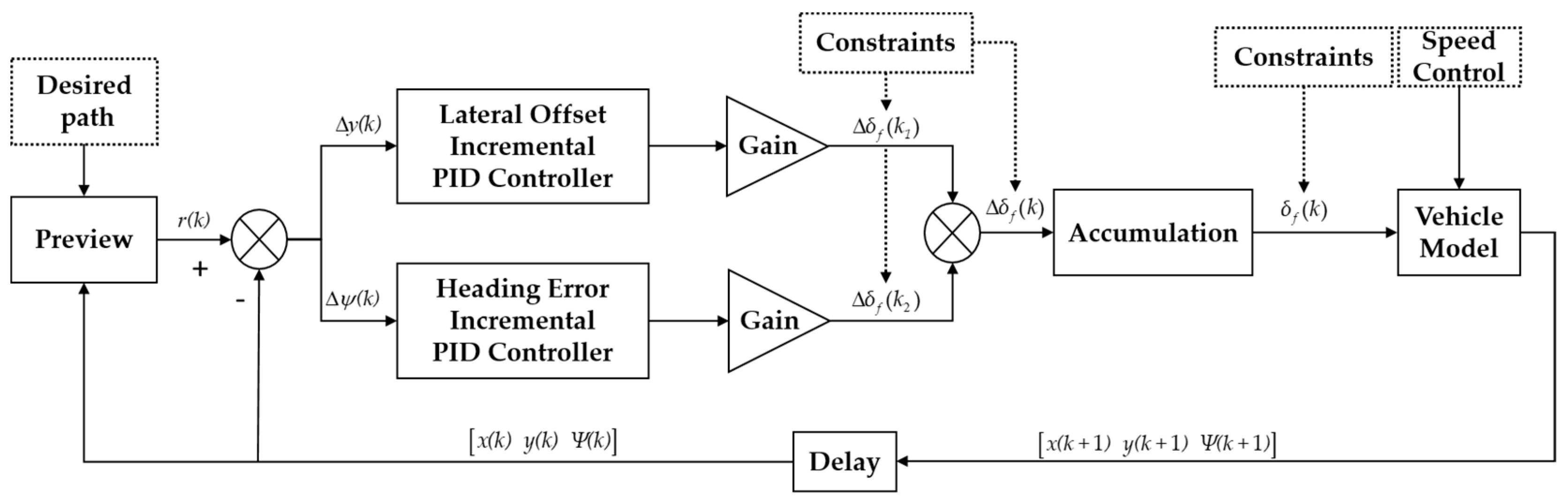
The failure modes of the 4WID electric vehicle system can be categorized as single wheel failure, opposite side double wheel failure, same side double wheel failure and multiple wheel failure. It is well known that if same side motor failure and multiple motor failures occur as the ultimate failure conditions for 4WID electric vehicles, we must take necessary precautions to brake the vehicles. This paper proposes the MIMO-MFAC active fault-tolerance method for the single wheel failure and opposite side-wheel failure conditions. All of the failure conditions of the drive system of 4WID electric vehicles are simulated and verified and the simulation time step is 0.01 s. When the drive system fails, the proposed method only utilizes the I/O data of the vehicle and uses a new dynamic linearization technique with a pseudo-partial derivative to correct the vehicle posture and to ensure that the vehicle maintains the desired values, thereby resulting in improved safety levels of the vehicles. Thus, the desired control objectives can be achieved by the coordinated adaptive fault-tolerant control of the drive and steering systems under all of the conditions illustrated below. Table 2, Table 3 and Table 4 display the maximum speed deviation, yaw rate and lateral position deviation, respectively, with or without control, under different working conditions. The results indicate that the proposed active fault-tolerant control method can ensure and improve vehicle safety, as well as enhance the longitudinal and lateral tracking ability under different failure conditions through cooperative fault-tolerant control of the drive and steering systems.
The simulation verification analysis of the active fault-tolerant control method under the typical condition, as displayed in Table 5, will be described in detail below.
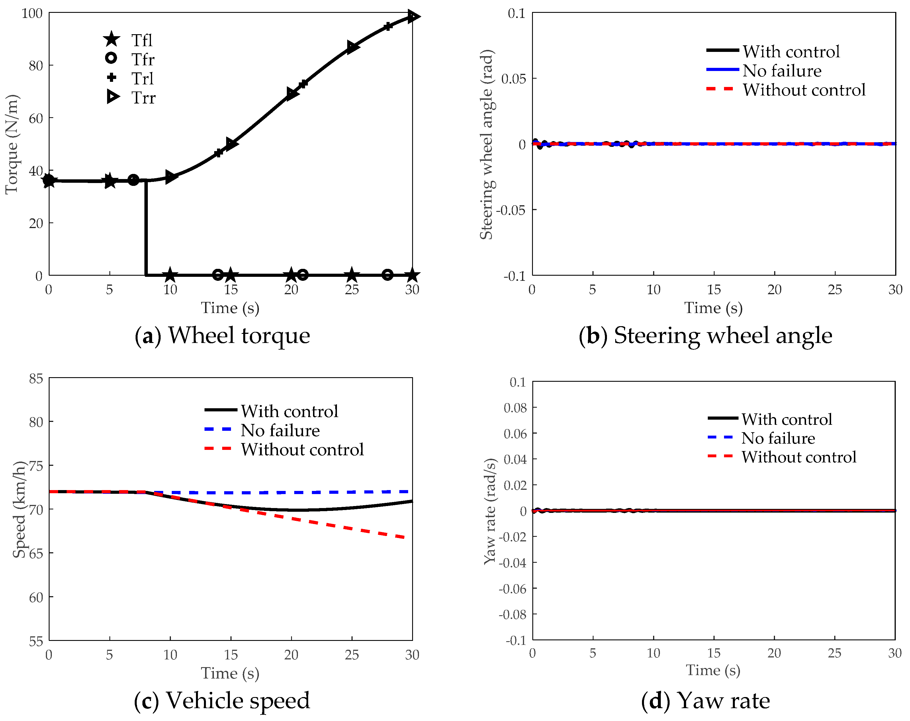
Condition F1: The vehicle is traveling at a constant speed and the expected speed is 72 km/h. At the 8th second, left front motor failure occurs.
The vehicle is traveling at a constant speed of 72 km/h in a straight-line condition and the left front motor fails at the 8th second. It is obvious from Figure 3e that the vehicle completely deviates from its trajectory without control, which easily induces traffic accidents. Moreover, under the control of the MIMO-MFA active fault-tolerant control algorithm proposed in this paper, when the left front wheel fails, the steering wheel illustrated in Figure 3b responds immediately. Furthermore, it decreases the normal wheel motor torques at the right front and rear and increases the normal wheel motor torques of the left rear, as illustrated in Figure 3a. Therefore, it ensures vehicle safety after the drive system fails and maintains the expected speed, as indicated in Figure 3c, so it does not deviate from the expected trajectory illustrated in Figure 3e.
We can also observe from Figure 3a,b that, during the entire fault-tolerant process, the adjustment ratio of the steering wheel angle is decreased with the drive system adjustment, thereby achieving the coordinated fault-tolerant result of the two systems. This provides an easy method for avoiding the overloading problem caused by using only the single actuator for fault tolerance after failure of the drive system and improving the vehicle safety. Table 6 below displays the vehicle speed and yaw rate and the later position deviation in the controlled and uncontrolled conditions after failure occurs.
Therefore, it can be concluded that the algorithm achieves the proposed active fault-tolerant result; moreover, this method can control the vehicle deviation within 10 cm and speed error within 3%.
Condition F2: The vehicle is traveling at a constant speed and the expected speed is 72 km/h. At the 8th second, left front and right front motor failure occur at the same time.
Without control, it is obvious from Figure 4c that the vehicle speed is reduced immediately when the motor fails but under the algorithm proposed in the paper, we can observe from Figure 4a that the controller increases the normal left rear and right rear motor torque to compensate for the lost motor torque of the left front and right front wheels. Therefore, it maintains the desired vehicle speed of 72 km/h, as the left front and right front wheels fail at the same time and the 4WID electric vehicle failure mode is the opposite side double-wheel failure. As illustrated in Figure 4b,d, no additional steering wheel angle and yaw rate are generated in the lateral direction. From the above analysis, the effectiveness of the designed controller designed is verified. The controller ensures that the vehicle can maintain the desired speed after failure of the drive system and will not allow deviation from the established path. Table 7 displays the vehicle speed, yaw rate and later position deviation with control or without control after failure occurs.
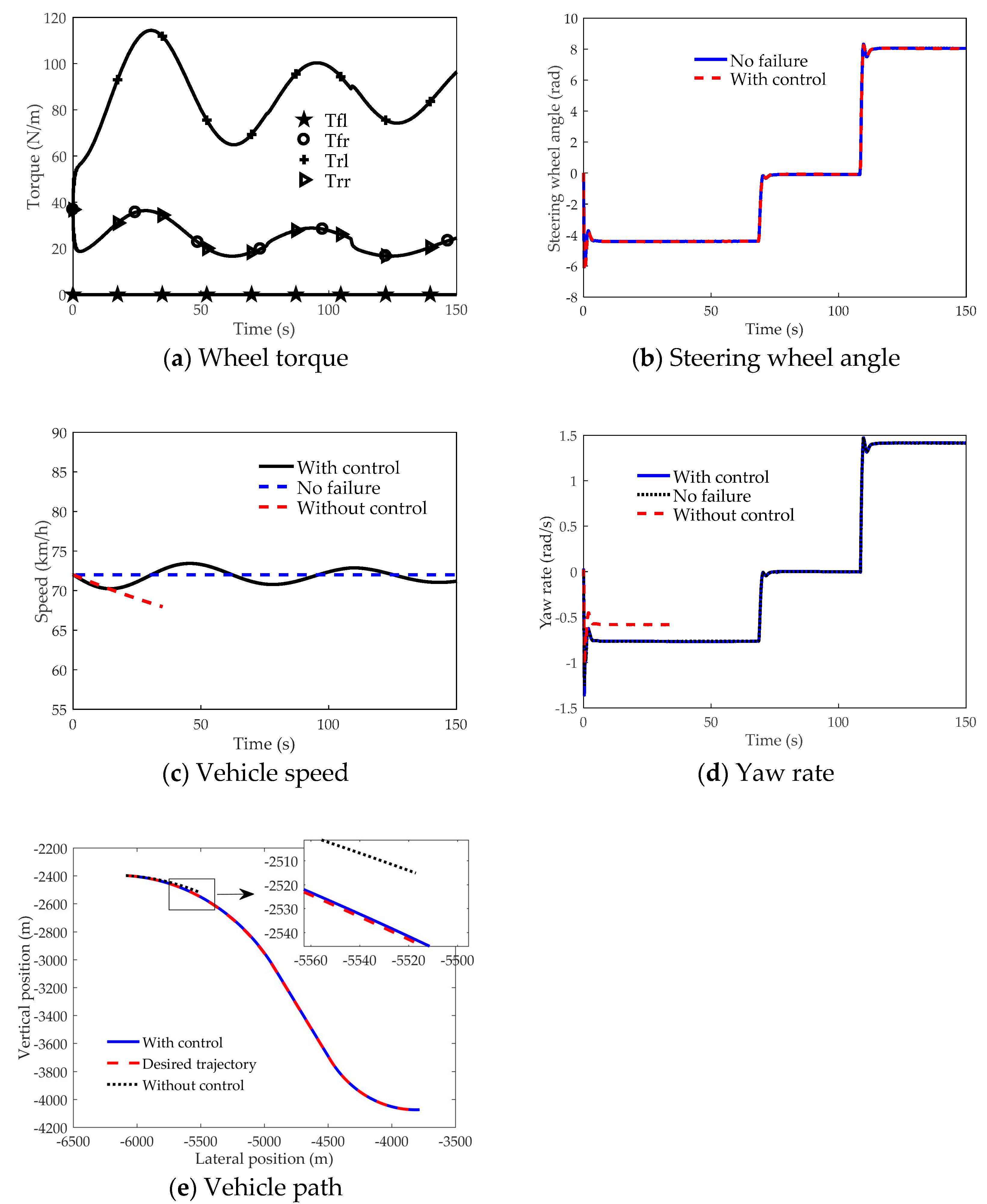
Condition F3: The vehicle is turning at a constant speed and the expected speed is 72 km/h. At the time of the 0th second, left front wheel failure occurs.
The vehicle turns at a constant speed of 72 km/h, as indicated in Figure 5c. At the 0th second, left front motor failure occurs. Without control, as indicated in Figure 5e, it is clear that the vehicle exhibits an obvious deviation; thus, it is likely to induce traffic accidents. When the left front wheel fails under the control of the proposed algorithm, the steering wheel responds immediately, as illustrated in Figure 5b. At the same time, as indicated in Figure 5a, the right front and right rear motor torques are reduced, while the left rear wheel motor torque is increased. Therefore, it is ensured that the vehicle safety can be improved and the desired vehicle speed can be maintained, as illustrated in Figure 5c and it does not deviate from the desired trajectory, as depicted in Figure 5d,e.
We can also observe from Figure 5a,b that, during the entire active fault-tolerant control process, with the addition of the wheel torque adjustment, the steering angle adjustment ratio is continuously reduced, thereby achieving cooperative fault-tolerant control of the drive and steering systems. This method can easily avoid the overload phenomenon caused by the single actuator after actuator failure and improve vehicle safety. Table 8 displays the vehicle speed, yaw rate and later position deviation with control or without control after failure of the drive system. We can conclude that the algorithm achieves the proposed active fault-tolerant results and the method can maintain the longitudinal speed error within 3% and lateral stability, thus improving the vehicle safety.

4.2. Experimental Verification

In order to verify the real-time algorithm performance, we used the driving simulator platform illustrated in Figure 6; five screens were positioned around the simulator vehicle, with three screens displaying the front traffic scenes and two displaying the back view. The CarSim software was embedded in the driving simulator to reflect the real vehicle movement features. In order to simulate real driving situations, the vehicle was supported by numerous hydraulic cylinders to achieve pitch, roll and yaw motions. For comparison with the simulation results, the vehicle model in CarSim was selected to be the same as in the simulation and the experimental testing conditions were designed almost the same as those in the simulation, as indicated in Table 9.
Experimental testing condition E1: The condition for a straight uniform speed is selected and the desired speed is set to 72 km/h, with single left front motor failure at the 0th second, as in the simulation. In this manner, we can conclude that, through the cooperative control of the drive system in Figure 7a and steering system in Figure 7b, the vehicles can maintain the expected speed, as indicated in Figure 7c, as well as the lateral ability, as illustrated in Figure 7d,e. Table 10 displays the vehicle speed, yaw rate and later position deviation with control or without control after failure of the drive system. It is demonstrated that the experimental verification results are similar to the simulation results. Moreover, in the driving simulator verification experiment, the system control period is less than 50 ms, so the verification of the control algorithm exhibits satisfactory real-time performance.
Experimental testing condition E2: The condition of straight uniform speed is selected; the desired speed is set to 72 km/h and drive motor failure at the opposite side is selected so that the left front motor and right front motor become completely ineffective at the 0th seconds. In this manner, we can conclude that, through the cooperative control of the drive system in Figure 8a and steering system in Figure 8b, the vehicle can maintain the expected speed, as indicated in Figure 8c, as well as the lateral ability, as illustrated in Figure 8d. Table 11 displaces the vehicle speed, yaw rate and later position deviation with control or without control after failure of the drive system. It is demonstrated that the experimental verification results are similar to the simulation results. Furthermore, in the driving simulator verification experiment, the system control period is less than 50 ms, so the verification of the control algorithm exhibits satisfactory real-time performance.
Experimental testing condition E3: The condition of a uniform turning speed is selected, the desired speed is set to 72 km/h and the single left front motor is selected to fail at the 0th second. When motor failure occurs at the 0th second, the remaining motor torque instantly increases and through the cooperative control of the drive system in Figure 9a and steering system in Figure 9b, the vehicles can maintain the expected speed, as indicated in Figure 9c, as well as the lateral ability, as illustrated in Figure 9d,e. Table 12 displaces the vehicle speed, yaw rate and later position deviation with control or without control after failure of the drive system. It is demonstrated that the experimental verification results are similar to the simulation results. Moreover, in the driving simulator verification experiment, the system control period is less than 50 ms, so the verification of the control algorithm exhibits satisfactory real-time performance.

5. Conclusions

In view of the failure of the 4WID electric vehicle drive system, this paper has proposed the MIMO-MFA active fault-tolerant control method, which does not rely on a system model and only uses system I/O data. Through the cooperative fault-tolerant control of the drive and steering system, vehicle safety of is guaranteed. In summary, the following conclusions can be drawn.
  • The proposed method of MIMO-MFA active fault-tolerant control can realize cooperative fault-tolerant control of the drive and steering systems under different failure conditions of 4WID vehicles, as well as improve vehicle safety. Moreover, it avoids using only a single actuator, such as the drive system or steering system, for fault-tolerant control under the limit condition, making it extremely easy for the motor to exceed the workload, thereby causing failure to complete fault-tolerant control successfully. Therefore, compared to the traditional fault-tolerant control method, the proposed method will make the entire control system more reasonable.
  • The control system design does not rely on an accurate system model; it only uses the system I/O data to solve the complex, nonlinear and uncertain effects of the vehicle system. Moreover, this method does not rely on the information of accurate fault diagnosis.
Furthermore, in the future, real-vehicle experiments will be carried out using the proposed control scheme.

Author Contributions

Conceptualization: Y.L.; Formal analysis: Y.H.; Investigation: F.J.; Methodology: Y.L. and Y.H.; Project administration: Y.L.; Visualization: F.J.; Writing—original draft: Y.H.; Writing—review and editing: R.C. and Y.W.

Funding

This research was funded in part by the International Science & Technology Cooperation Program of China, under grant No. 2016YFE0102200 and in part by the State Program of the National Natural Science Foundation of China, under grant 51575295.

Conflicts of Interest

The authors declare no conflict of interest.

References

  1. Veillette, R.J. Reliable linear-quadratic state-feedback control. Automatica 1995, 31, 137–143. [Google Scholar] [CrossRef]
  2. Yang, G.H.; Wang, J.L.; Soh, Y.C. Reliable LQG control with sensor failures. IEE Proc. Control Theory Appl. 2000, 147, 433–439. [Google Scholar] [CrossRef]
  3. Hess, R.A.; Wells, S.R. Sliding mode control applied to reconfigurable flight control design. J. Guid. Control Dyn. 2003, 26, 452–462. [Google Scholar] [CrossRef]
  4. Kazemi, R.; Janbakhsh, A.A. Nonlinear adaptive sliding mode control for vehicle handling improvement via steer-by-wire. Int. J. Automot. Technol. 2010, 11, 345–354. [Google Scholar] [CrossRef]
  5. Alwi, H.; Edwards, C. Fault tolerant control using sliding modes with on-line control allocation. Automatica 2008, 44, 1859–1866. [Google Scholar] [CrossRef] [Green Version]
  6. Ho, L.; Yen, G.G. Reconfigurable control system design for fault diagnosis and accommodation. Int. J. Neural Syst. 2002, 12, 497–520. [Google Scholar] [CrossRef] [PubMed]
  7. Polycarpou, M.M. Fault accommodation of a class of multivariable nonlinear dynamical systems using a learning approach. IEEE Trans. Autom. Control. 2001, 46, 736–742. [Google Scholar] [CrossRef]
  8. Wang, R.; Wang, J. In-Wheel Motor Fault Diagnosis for Electric Ground Vehicles. In Proceedings of the ASME 2010 Dynamic Systems and Control Conference, Cambridge, MA, USA, 12–15 September 2010; pp. 133–140. [Google Scholar]
  9. Kawakami, K.; Matsugaura, S.; Onishi, M. Development of fail-safe technologies of ultra high performance EV “KAZ”. In Proceedings of the 18th International Electric Vehicle Symposium (EVS-18), Berlin, Germany, 20–24 October 2001. [Google Scholar]
  10. Mutoh, N.; Takahashi, Y. Front-and-rear-wheel-independent-drive type electric vehicle (FRID EV) with the outstanding driving performance suitable for next-generation adavanced EVs. In Proceedings of the 2009 IEEE Vehicle Power and Propulsion Conference, Dearborn, MI, USA, 7–10 September 2009; pp. 1064–1070. [Google Scholar]
  11. Mutoh, N.; Nakano, Y. Dynamics of Front-and-Rear-Wheel-Independent-Drive-Type Electric Vehicles at the Time of Failure. IEEE Trans. Ind. Electron. 2012, 59, 1488–1499. [Google Scholar] [CrossRef]
  12. Wang, R.; Wang, J. Actuator-Redundancy-Based Fault Diagnosis for Four-Wheel Independently Actuated Electric Vehicles. IEEE Trans. Intell. Transp. Syst. 2014, 15, 239–249. [Google Scholar] [CrossRef]
  13. Wang, R.; Wang, J. Fault-Tolerant Control with Active Fault Diagnosis for Four-Wheel Independently Driven Electric Ground Vehicles. IEEE Trans. Veh. Technol. 2011, 60, 4276–4287. [Google Scholar] [CrossRef]
  14. Li, D.; Song, Y.; Huang, D.; Chen, H. Model-Independent Adaptive Fault-Tolerant Output Tracking Control of 4WS4WD Road Vehicles. IEEE Trans. Intell. Transp. Syst. 2013, 14, 169–179. [Google Scholar] [CrossRef]
  15. Hou, Z.; Jin, S. Data-driven model-free adaptive control for a class of MIMO nonlinear discrete-time systems. IEEE Trans. Neural Netw. 2011, 22, 2173–2188. [Google Scholar] [PubMed]
  16. Hou, Z.; Jin, S. A novel data-driven control approach for a class of discrete-time nonlinear systems. IEEE Trans. Control Syst. Technol. 2011, 19, 1549–1558. [Google Scholar] [CrossRef]
  17. Hou, Z.; Jin, S. Model Free Adaptive Control: Theory and Applications; Brain Research; CRC press: Boca Raton, FL, USA, 2016; Volume 281, pp. 202–205. [Google Scholar]
  18. Dos Santos Coelho, L.; Coelho, A.A.R. Model-free adaptive control optimization using a chaotic particle swarm approach. Chaos Solitons Fractals 2009, 41, 2001–2009. [Google Scholar] [CrossRef]
  19. Li, Z.; Ding, Z.; Wang, M.; Oko, E. Model-free adaptive control for MEA-based post-combustion carbon capture processes. Fuel 2018, 224, 637–643. [Google Scholar] [CrossRef]
  20. Tan, K.K.; Lee, T.H.; Huang, S.N.; Leu, F.M. Adaptive-predictive control of a class of SISO nonlinear systems. Dyn. Control 2001, 11, 151–174. [Google Scholar] [CrossRef]
Figure 1. Architecture of MIMO-MFA active fault-tolerant control method.
Applsci 09 00276 g001
Figure 2. Architecture of path tracking controller.
Applsci 09 00276 g002
Figure 3. Simulation comparison with/without control under F1 condition.
Applsci 09 00276 g003
Figure 4. Simulation comparison with/without control under F2 condition.
Applsci 09 00276 g004
Figure 5. Simulation comparison with/without control under F3 condition.
Applsci 09 00276 g005
Figure 6. Driving simulator platform.
Applsci 09 00276 g006
Figure 7. Experimental comparison with/without control under E1 condition.
Applsci 09 00276 g007
Figure 8. Experimental comparison with/without control under E2 condition.
Applsci 09 00276 g008
Figure 9. Experimental comparison with/without control under E3 condition.
Applsci 09 00276 g009
Table 1. Main parameters of vehicle.
ParameterSymbolValue
Sprung mass (kg)m2257
Front axle distance to COG (m)a1.33
Rear axle distance to COG (m)b1.616
Tire radius (m)d0.7902
Front wheel total lateral stiffness (N/deg)k1−1317.81
Rear wheel total lateral stiffness (N/deg)k2−1317.81
Table 2. Maximum speed deviation with or without control (km/h).
Driving ConditionFailure ConditionWithout ControlWith Control
Uniform linear motionSingle wheel2.751.2019
Opposite side wheel5.37942.121
Uniform steering motionSingle wheel11.68231.811
Opposite side wheel12.54432.5822
Table 3. Maximum yaw rate deviation with or without control (rad/s).
Driving ConditionFailure ConditionWithout ControlWith Control
Uniform linear motionSingle wheel0.2240.002
Opposite side wheel0.00130.0012
Uniform steering motionSingle wheel0.35820.0444
Opposite side wheel0.08350.0625
Table 4. Maximum deviation of lateral with or without control (m).
Driving ConditionFailure ConditionWithout ControlWith Control
Uniform linear motionSingle wheel15.53120.0964
Opposite side wheel0.06340.05
Uniform steering motionSingle wheel27.90770.58
Opposite side wheel0.1580.125
Table 5. Special condition of simulation verification.
ConditionDriving ConditionFailure Condition
F1Uniform linear motion 72 km/hLeft front wheel failure
F2Uniform linear motion 72 km/hLeft front and right front wheel failure
F3Uniform steering motion 72 km/hLeft front wheel failure
Table 6. Statistical control effect under F1 condition.
ItemWithout ControlWith Control
Maximum yaw rate deviation (rad/s)0.2240.002
Maximum speed deviation of speed (km/h)2.751.2019
Maximum lateral deviation/(m)15.53120.0964
Table 7. Statistical control effect under F2 condition.
ItemWithout ControlWith Control
Maximum speed deviation (km/h)5.37942.121
Maximum yaw rate deviation (rad/s)0.00130.0012
Table 8. Statistical control effect under F3 condition.
ItemWithout ControlWith Control
Maximum yaw rate deviation (rad/s)0.35820.0444
Maximum speed deviation (km/h)11.68231.811
Maximum lateral deviation /(m)27.90770.58
Table 9. Special conditions of experimental verification.
ConditionDriving ConditionFailure Condition
E1Uniform linear motion 72 km/hLeft front wheel failure
E2Uniform linear motion 72 km/hBoth left and right wheel failure
E3Uniform steering motion 72 km/hLeft front wheel failure
Table 10. Statistical control effect under E1 condition.
ItemWithout ControlWith Control
Maximum yaw rate deviation (rad/s)0.2240.003
Maximum speed deviation (km/h)2.751.1422
Maximum lateral deviation /(m)15.53120.0548
Table 11. Statistical control effect under E2 condition.
ItemWithout ControlWith Control
Maximum yaw rate deviation (rad/s)00
Maximum speed deviation (km/h)5.36882.5787
Maximum lateral deviation /(m)00.08
Table 12. Statistical control effect under E3 condition.
ItemWithout ControlWith Control
Maximum yaw rate deviation (rad/s)0.35820.1895
Maximum speed deviation (km/h)11.68233.5738
Maximum lateral deviation /(m)27.90770.52

