Approach of Coordinated Control Method for Over-Actuated Vehicle Platoon based on Reference Vector Field


1
State Key Laboratory of Automotive Simulation and Control, Jilin University, Changchun 130012, China
2
School of Engineering, University of Lincoln, Lincoln LN6 7TS, UK
3
School of Automobile and Traffic Engineering, Liaoning University of Technology, Jinzhou 121001, China
*
Author to whom correspondence should be addressed.
Appl. Sci. 2019, 9(2), 297; https://doi.org/10.3390/app9020297
Submission received: 30 November 2018
/
Revised: 17 December 2018
/
Accepted: 9 January 2019
/
Published: 15 January 2019
(This article belongs to the Special Issue Multi-Actuated Ground Vehicles: Recent Advances and Future Challenges)
Abstract
:Featured Application
The proposed method is applied to the coordinated control for over-actuated vehicle platoon with an integrated hierarchical controller.
Abstract
Collaborative vehicle platoon control with full drive-by-wire vehicles with four-wheel independent driving and steering (FWIDSV) has attracted broader research interests. However, the problem of cooperative vehicle platoon control in two-dimensional driving scenes remains to be solved. This paper proposes a coupling control method for path tracking and spacing-maintaining based on the reference vector field (RVF). An integrated hierarchical control structure, including the following control layer, tire force allocator layer, and an actuator controlling layer for FWIDSV is presented. Inside, the next control layer was designed according to the spacing control strategy and RVF within the limitation of the friction circle. For verifying the effectiveness of this control method, sufficient conditions for error convergence are analyzed when considering the influence of the critical parameters on the particle dynamics model. The tire force allocator layer is designed based on linear quadratic programming (LQP), which is used to distribute the total forces and yaw moment. The sliding mode control (SMC) is employed to track the desired tire forces in the actuator controlling layer. The proposed control methods are validated through simulation in intelligent cruise control (ICC) and platoon merging scenarios. The results demonstrate an effective FWIDSV platoon control approach that is based on the RVF in the 2-D driving scenes.
1. Introduction
With the development of intelligent connected technology and vehicle automation technology, intelligent vehicle and multi-vehicle collaborative control have attracted considerable research interests. Vehicle platoon enables multiple vehicles to drive in a formation by automatically adjusting the spacing between the cars. By maintaining a reasonable distance and yaw angle between the adjacent cars, the “traction effect” in aerodynamics can effectively save energy and reduce pollutant emissions [1]. Besides, platoon control can increase traffic capacity and reduce the probability of traffic accidents, which was demonstrated in many studies [2,3,4]. These potential advantages have led to an increasing emphasis on the research of intelligent connected vehicle collaborative control.
With the improvement of platoon automation, considerable researches efforts were devoted to the development of collaborative platoon control in 2-D driving scenes. In 2006, Maziar E. Khatir proposed an adaptive cruise control method for path tracking and the side-by-side driving control through the sixth-order dynamics model, and the performances of the front-wheel steering vehicle and the rear-wheel steering vehicle were compared as a following vehicle [5]. In Cristorfer Englund’s study, a robust proportion-integral-derivative (PID) control system was established based on the vehicle dynamics model, which combines path tracking and speed matching to achieve longitudinal and lateral coordinated control [6]. Chen Chang created a three-degree-of-freedom (3-DOF) nonlinear dynamic model, including engine, clutch, automatic transmission, and tire model. The sliding mode control (SMC) controller was designed to test the control effect of the platoon through acceleration and steering driving situations [7]. T. FUJIOKA developed a longitudinal SMC controller to maintain a fixed distance between vehicles and to ensure platoon stability, and the finite state machine was used to realize the conversion of the vehicle controlling state in complicated situations [8]. In Zhibin Shuai’s research, the vehicle’s longitudinal and lateral motions were controlled by adaptive fuzzy SMC and it showed good performance [9]. Spacing control of platoon has been intensively investigated, but it remains challenging to develop a path following method for platoon control. Additionally, the above studies are all aimed at traditional front-wheel steering vehicles, while the dynamics characteristics of four-wheel independent driving and steering (FWIDSV) are not considered in platoon control. As a kind of over-actuated vehicle, FWIDSV can control the driving torques and steering angles of front and rear wheels separately, thus can effectively improve the steerability performance and handling stability [10]. As an actuator redundancy system, the primary challenge is dealing with the physical constraints and the actuator redundancy. Most of the solutions are considering it as an optimization problem; therefore, model predictive control theory (MPC) and linear quadratic programming (LQP) are used in tire force allocation [11]. Other studies focus on the pseudo inverse algorithm and design it for dynamically allocating the desired external yaw moment into the redundant tire actuators because of its faster calculation [12].
In 2002, T J Gordon proposed a driver model for self-driving vehicles based on the convergent vector field. By establishing a reference vector field (RVF), non-linear feedback control and residual friction control were used to ensure that the vehicle’s driving direction converges to the reference path, and pointed out the application prospect in advanced cruise control systems [13]. Since then, the reference vector field method has been widely studied and applied in the fields of path planning and tracking, obstacle avoidance, and extremum seeking [14,15,16].
In conclusion, when RVF was used as the motion controller of the vehicle, the flow vector field can be constructed by the look-ahead point, the reference path, and the current position to provide the desired force and moment for the vehicle. When compared with other controllers, like MPC and PID controller, RVF could be considered as an optimal solution when following a leading vehicle, so it is much faster and easier to get the optimal solution. Besides, it is more suitable for the FWIDSV, which can decouple the total force and control the tires independently. In the multi-vehicle platoon and adaptive cruise control, the direction of movement of the following vehicle points to the balanced point between the leading vehicle and the following vehicle. The reference vector field can be constructed according to the leading vehicle, the balanced point, the reference trajectory, and the geometric relationship for the following vehicle, so that it can ensure the maintenance of a reasonable distance from the leading vehicle by following the trajectory. It might improve the automation of platoon control by coupling lateral and longitudinal motion.
This paper explores a new approach to solve the coupling vehicle platoon control problem of the path tracking. Several contributions have been made in this paper and structured, as follows. Section 2 analyzes the particle dynamics and reference vector field. The sufficient conditions for the error convergence are discussed, which can ensure the following vehicle’s trajectory to converge to the reference path of the leading vehicle. In Section 3, the integrated controller is built within the following control layer, tire force allocator layer, and actuator control layer. The simulating validations are constructed in Section 4, in which the intelligent cruise control and platoon merging situations are set to verify the response characteristics of FWIDSV with the integrated controller. In Section 5, the mean contributions are summarized in the article, and the possible application fields and development trends are discussed.
2. Reference Vector Field of Vehicle Following
2.1. Spacing Control Strategy of Platoon
The control objective of the platoon is to ensure the consistency of the vehicles while maintaining the desired distance between adjacent vehicles. Among them, the calculation strategy of the inter-vehicle distance is called the spacing control strategy. The expecting position of the following vehicle, as determined by spacing control strategy at the current moment, is called the balanced point. When extending the one-dimensional platoon control to two-dimensional, the following vehicle is required to track the path of the leading vehicle while maintaining the longitudinal spacing at the same time. There are two central control strategies when performing lateral platoon control, including direct vehicle-following and vehicle path-following. The path-following has some advantages over direct vehicle-following [17]:
- (1)
- In the path-following strategy, the position of the following vehicle can be represented by the distance in the path coordinate system relative to the leading vehicle. The interaction between followers is reduced based on this strategy. Therefore, the control error will not be amplified with the transmission of the platoon, which weakens the importance of platoon stability.
- (2)
- The relative heading angle of the preceding vehicle is hard to measure, which means that the following vehicle cannot get enough and proper information for direct vehicle-following.
- (3)
- It is much easier for the path-following strategy to modify the feedback input to improve the following performance. The reference path can be replanted according to the surround information and traffic rules.
- (4)
- The path-following strategy requires that the path information of leading vehicle should be saved and updated in following vehicle’s controller. When compared with the path-following approach, the direct vehicle-following strategy needs less data, so it is more suitable for the sample driving condition, like longitudinal following condition.
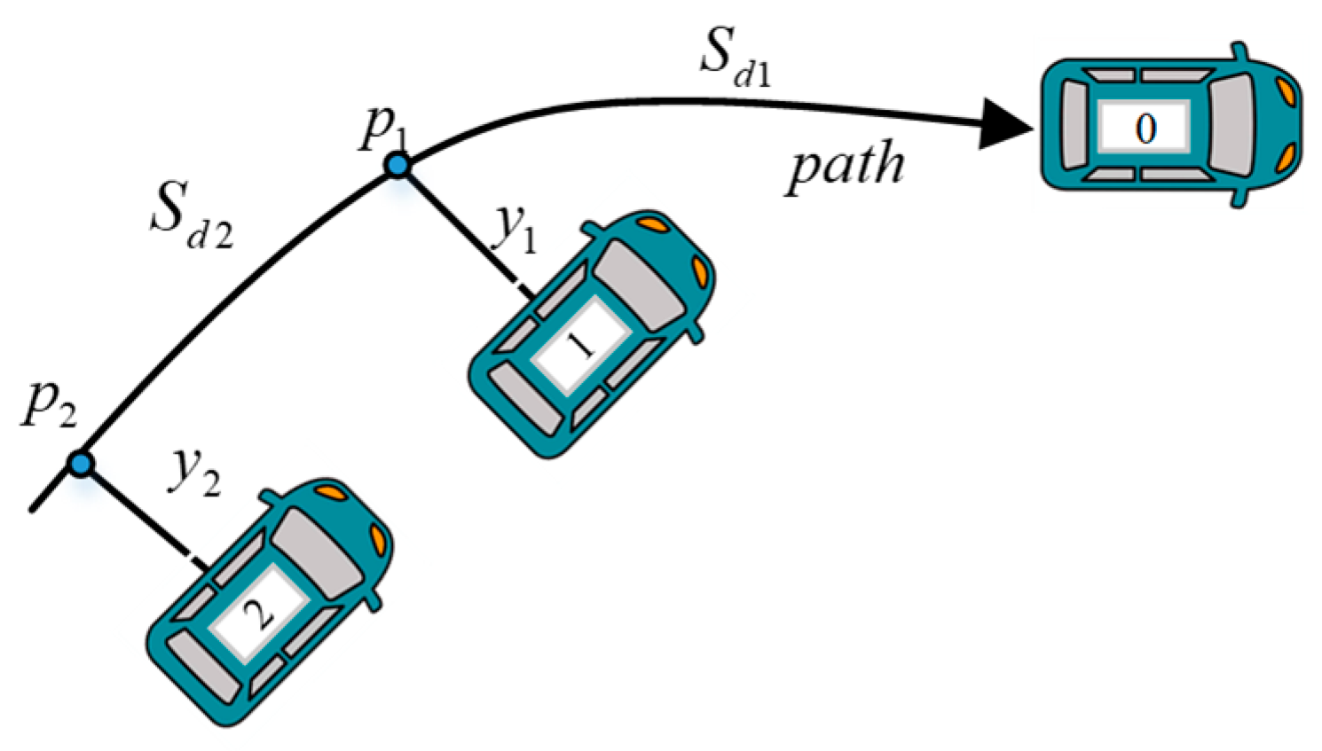
With these advantages, the path following strategy is selected in this paper. To facilitate the analysis of the positional relationship during the two-dimensional movement of the platoon, the path-following strategy is as shown in Figure 1. Sd is the expecting distance between the leading vehicle and balanced point. Taking the closest position of the following vehicle i as p(xgi), then S is the distance between p(xgi) and its stable point; yi denotes the distance between the position of vehicle i and the point p(xgi).
2.2. Particle Dynamic Model and Reference Vector Field
Vehicle motion is simplified in a 2-D plane, and the vehicle is considerate as a single particle. At this point, the particle has two degrees of freedom in the plane, including the longitudinal direction and lateral direction. Since the acceleration of the vehicle is limited by road adhesion, the control variable u(t) of the vehicle particle dynamics model is selected as acceleration, and the particle dynamics model can be simplified, as shown in formula (1), where xG and vG are 2-D vectors.
As is shown in Figure 2, the following flow vector w was built by following vehicle’s position and the balanced point. The integration of the vector forms a streamline that converges on the reference path. The tangent direction of each point on the streamline is the same as the vector w. R denotes the distance between the current position of the following vehicle and its balanced points. There is a flow vector that is associated with the current position of the following vehicle, regardless of whether the following vehicle is on either side of the path, and the vector w could be described as formula (2).
Apparently, when the leading vehicle is traveling in a straight line, there is .
The value of v is the norm of the vehicle speed vector, which can be selected as a fixed value when the path tracking control is performed separately; in the coordinated control of the platoon, v should be consistent with the speed of other intelligent vehicles in the platoon. To ensure that the distance between vehicles meets the requirements of the spacing control strategy, the value of v should be chosen carefully. The calculation method used in this paper is as shown in (3).
where V0 is the speed vector of the leading vehicle. According to (2), the curve that is formed by the integration of the flow vector has the relationship as is shown in (4).
To obtain a general solution to the differential Equation (4), the expression of the curve can be obtained as is shown in (5).
There is an initial error between the desired velocity vector determined by the flow vector and the actual velocity vector of the particle at the current location, as shown in (6).
To make the following vehicle’s path converge to the reference path of the leading vehicle, the following vehicle’s driving direction tends to the course of the streamline. Differentiate the (6) and (7) can be obtained.
where , .
- (1)
- Assuming that the initial error vector e is 0, the error can be kept at 0 by controlling value u1.
- (2)
- Assuming that the initial error vector e is not 0, thenwhere the first item of control u is based on the position feedback information of the vehicle, and the second item is used to eliminate the initial error. The usage of the friction circle is as shown in Figure 3.
To prevent the control variable from exceeding the limitation of the friction circle, there is a restriction, as shown in (10).
Based on the previous analysis and requirements, the control law for eliminating the error between the vehicle speed and the flow vector is constructed:
When the error is small enough, the use of the tire force can be reduced to make the vehicle converge to the path stably, so v0 is introduced as a judgment condition.
It can be seen from the analysis that the convergence time of the error is related to the use of the tire force. This paper numerically simulates different values of ε (the value of ε is defined between 0~μg, where μ is considered as 1.0 and g denotes the gravity acceleration, which is selected as 9.8 m/s2). The leading vehicle is driving along with a straight line—y = 0, while the initial position of the following vehicle is (0, −3). The results of numerical simulations are as shown in Figure 4.
As shown in Figure 4a, when the particle model is tracking the flow vector, the value of control law is used to eliminate the error between the actual vehicle speed and the streamline vector. If the tire force is insufficient, the error convergence speed will be small. As a result, the vehicle will oscillate around the reference path. As the ε increases, the oscillation amplitude and the error convergence speed increase gradually, and the overshoot gradually decreases. As can be seen in Figure 4b, the value of ε has a particular influence on the longitudinal spacing control. Moreover, as the utilization of the friction circle increases, the longitudinal spacing converges more rapidly and stably.
For theoretical analysis about the influence of ε on the convergence speed of the error between the velocity vector and the reference vector, Equation (9) is differentiated to obtain the Jacobian matrix H, and its eigenvectors are m1 and m2.
Let e be the norm of the error vector e, then (12) is obtained from the (7).
There is , (13) could be obtained with the combination of (7) and (12).
When m1 + m2 = 0, the streamline does not converge currently, and there is a maximum derivative of error convergence, as shown in (14).
Since the derivative of the error is bounded, when there is an initial error e > 0, the error will decrease to 0 within a finite time τ, where the magnitude of τ is as shown in (15). The results are in good consistent with the observed Figure 4.
2.3. Sufficient Conditions for Following Errors’ Convergence
In addition to the influence of the friction circle on the path tracking and the spacing control, the parameter k in Equation (3) also affects the perspective of subjective guessing. To explore the k’s influence on the error convergence of the trajectory and spacing, the same numerical simulation scenario as in 2.2 is used, and different control gain values are applied. The result is shown in Figure 5. It can be found from Figure 5 that, in the step input, the overshoot will increase when the error is enhanced with the increase of k. When k ≤ 0.2, the overshoot is eliminated; Figure 5 b shows the longitudinal spacing error. The convergence speed becomes faster as k increases, and when k = 0, the norm of the flow vector w is directly related to the speed of the leading vehicle. At this time, the current error can only be prevented from further enlarging, but the error will not converge. Therefore, the selection of k is a contradictory parameter for the convergence of trajectory tracking error and the longitudinal following error. Two tracking targets should be coordinated in the application.
To explore the conditions that enable the following vehicle to converge to the balanced point when the leading vehicle drives in a stable driving state (longitudinal uniform speed), this paper constructs a smooth positive function related to the distance between the vehicle and the balanced point, as shown in Figure 6. The expressions of R(x) is as shown in (16). xl denotes the position vector of balanced point and xg denotes the position vector of the following vehicle.
To make as , R(xg) is required to monotonically decrease. When , there is .
Assuming that , and the leading vehicle is in a stable and uniform straight-line driving state, the component of the speed in the path direction is zero. Suppose that the position of the vehicle at time t1 is xg1 and the position at time t2 is xg2, then R(xg) is asked to satisfy Equation (17).
where .
According to the previous analysis, the conditions that the error function trends to zero needs to satisfy:
(1) the flow vector converges to the balanced point in the reference trajectory;
(2) the error between the vehicle speed and the flow vector is bounded;
(3) the controlled variable-the acceleration is limited by the friction circle; and,
(4) the control gain k is greater than zero.
The above conditions need to be satisfied at the same time to ensure that the following vehicle gradually approaches the balanced point.
3. Dynamic Model and Integrated Controller of FWIDSV
To verify the practical performance of FWIDSV with the reference vector field as the following vehicle, the 3-DOF FWIDSV dynamics model and integrated controller are used in this section to describe the motion of FWIDSV. The control structure of FWIDSV is as shown in Figure 7. The desired lateral and longitudinal total force of the vehicle is obtained from the following control layer, and the desired yaw moment is obtained by the SMC. The tire force allocator layer uses LQP to decouple the total force and moment, and the tire force of each wheel are obtained. The desired tire force is achieved by the actuator control layer by controlling the tire steering angles and the driving torques.
3.1. Following Control Layer
The ideal aX and aY in the global coordinate system can be obtained from the RVF in the previous discussion. To obtain the total longitudinal and lateral forces of the vehicle in vehicle coordinates, the coordinate system is converted by Equation (18).
where φ denotes the yaw angle of the vehicle; axd and ayd are desired longitudinal acceleration and lateral acceleration in vehicle coordinate system.
When controlling the yaw moment of the vehicle, it is necessary to consider the tracking error of the yaw angle. In this paper, the ideal yaw moment is obtained by SMC. The non-singular interrupted sliding surface is adapted to ensure that the tracking error can converge in the effective time on the interrupted sliding surface and it has fast and high-precision response characteristics [18]. The structural sliding surface s is as shown in the (19).
where . α and β denote the positive constant; p and q are the positive odd number, which satisfies that .
The calculation method of Mz is as shown in the (20), in which η determines the approach rate of the system state on the sliding surface; Φ can smooth the chattering phenomenon in the control process. The controller parameters are shown in the Table 1.
3.2. Tire Force Allocator Layer
To facilitate the two-dimensional dynamic modeling and analysis of the vehicle, the following rationalization assumption is made: the road surface is flat, and the vertical motion of the vehicle is ignored.
The schematic diagram of FWIDSV is shown Figure 8. The meanings of the symbols are as shown in Table 2.
According to Newton’s second law, the balanced force equations of the vehicle along the x-axis, y-axis, and z-axis are obtained, as shown in (21).
where
As a redundant system, the dynamics model of FWIDSV has three degrees of freedom but it has eight controllable variables, including the lateral and longitudinal forces of each wheel in FWIDSV. The forces and moments output in the following control layer are distributed to four wheels for specific optimization purposes. LQP and pseudo-inverse are used to solve the math calculation in the most studies of the tire force distribution [11,12]. In this paper, LQP is introduced to distribute the tire force, as it is easier to solve optimization problems and add constraints. The objective function is shown in (22).
To solve the tire force through LQP, the optimization function needs to be converted into a standard form, as shown in (23).
Let matrix G and matrix in linear quadratic programming be
Proof:
When using LQP in tire force allocator layer, the lateral and longitudinal forces of the tires need to meet the limits of the friction circle. However, it is quite tricky and time consuming to use it as a nonlinear constrained optimizing problem. As shown in Figure 9, this paper adopts the linear polygon constraint method to simplify the nonlinear friction circle constraint [19], and the specific constraint is shown in (26).
3.3. Actuator Controller
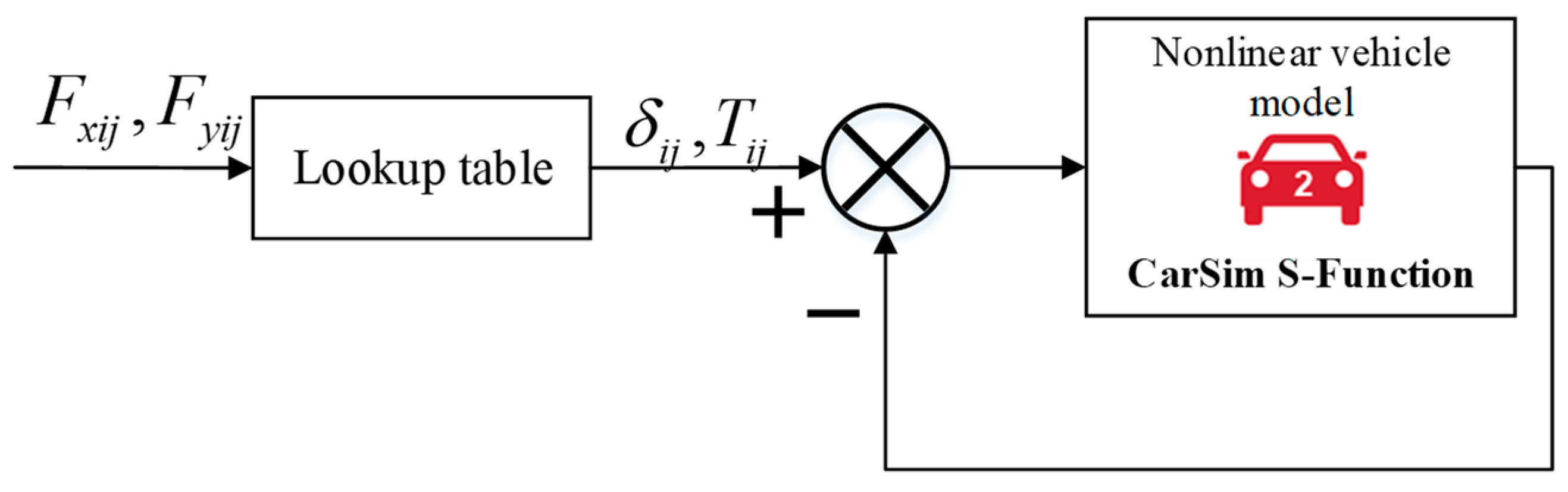
Actuator control layer of the FWIDSV is designed to obtain the desired tire force. The longitudinal and lateral forces of the tire are affected by the nonlinear deflection characteristics, respectively. Many methods for obtaining tire torque and wheel angle through the desired tire force include the linear tire force model [20], the non-linear Dugoff tyre model [12,21], magic tire model, and so on [22]. Information flow in Figure 10 shows the working principle of the actuator controlling layer.
4. Simulation Validation
A relatively brief set of simulations is presented with the aim of testing the feasibility of the reference flow vector and assessing the proximity between the dynamics model of FWIDSV and particle model. This section will focus on the convergence of the longitudinal error and the path tracking ability of the FWIDSV platoon under different scenarios.
The controllers are built in the Matlab/Simulink environment, and CarSim is used for the dynamic simulation. Two simulation cases, including ICC (Intelligent cruise control) and platoon merge maneuvers are conducted in this section. A high-fidelity B-class hatchback model is selected and modified into a FWIDSV, the inputs variables of which are steering angles and wheel torques. Assuming that the vehicle has a vehicle-to-vehicle communication function and sensor detection device, the following vehicle can obtain the speed of the leading vehicle and the path information. The key parameters of the FWIDSV are listed in the Table 3.
4.1. Intelligent Cruise Control of Single Following Vehicle
The cooperative control of the intelligent connected vehicle was developed by the adaptive cruise system (ACC). With the integration of the ACC and the LKS, some automotive companies developed and launched the traffic jam assistance system (TJA), also called ICC system. The particle model is compared with the FWIDSV model under the same control parameters, and a more realistic dynamic response verifies the effectiveness of the reference vector field control, tire force allocator, and actuator control layer.
As can be seen from parts (a) and (b) of Figure 11, the performance of the FWIDSV is worse than the ideal particle dynamics model, including the overshoot and tracking convergence speed and longitudinal spacing convergence speed while following a leading vehicle. This is understandable because of the nonlinear characteristics of the FWIDSV. It must also be mentioned that the error of lateral path tracking and spacing flowing still tend to zero, which proves the effectiveness of the controller.
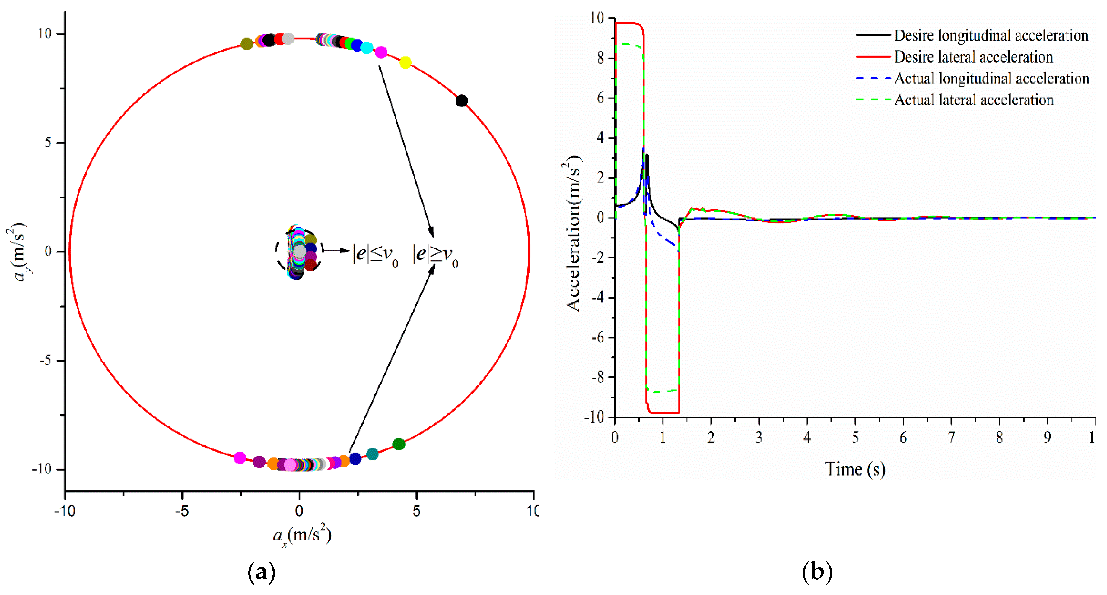
In Figure 12a, the ideal vehicle accelerations determined in the reference vector field are listed as discrete points. The acceleration is mainly distributed above, below, and the center of the friction circle, which is determined by ε, v0, and the specific working conditions. When |e|≤v0, using ε as much as possible will make the vehicle less prone to stability. Figure 12b shows the performance of the FWIDSV under tire force distribution and control layer control and it demonstrates that, when the initial error e is larger, the larger tire force is used to track the path and longitudinal spacing. However, after the error is reduced, the use of tire force is stabilized at around zero. In summary, the reference vector field and the FWIDSV integrated controller can guarantee the stable and reliable tracking of the path and the preceding vehicle by FWIDSV under this condition.
To verify the control effect of the actuator control layer, the desired accelerations of FWIDSV and the actual acceleration are compared. It can be seen from the Figure 12b that, through the direct integrated control of the FWIDSV wheel angle and torque, the actual acceleration response of the vehicle conforms to the changing trend of the desired acceleration. However, due to reasons, such as reasonable simplification or difficulty in modeling, there is a reasonable deviation between the two. The main reason is that in the calculation of the ideal acceleration, factors, such as resistance, are not considered. To more intuitively display the control process of the execution layer, the torque and steering angle of the FWIDSV are as shown in Figure 13.
4.2. Intelligent Cruise Control in Curve Road
To verify the effectiveness of the proposed control method in the two-dimensional driving scene, the leading vehicle will travel in a curve with a length of 200 m and the following vehicle is controlled according to the preset spacing and the trajectory of the leading vehicle. The initial longitudinal spacing of the following car and the navigator is 5m, while the desired spacing is 4m. Therefore, the initial distance (initial longitudinal tracking error) of the following vehicle and its balance point is 1 meter.
It can be seen from Figure 14a that the following vehicle’s trajectory is basically the same as the leading vehicle’s, indicating that, under the control of the RVF, the following vehicle can achieve lateral control accurately, so that it can travel on the path of the leading vehicle. Figure 14b shows that the following vehicle reaches the stable point in about 2s, and the inter-vehicular distance is guaranteed by real-time control.
4.3. Merging of the Platoon
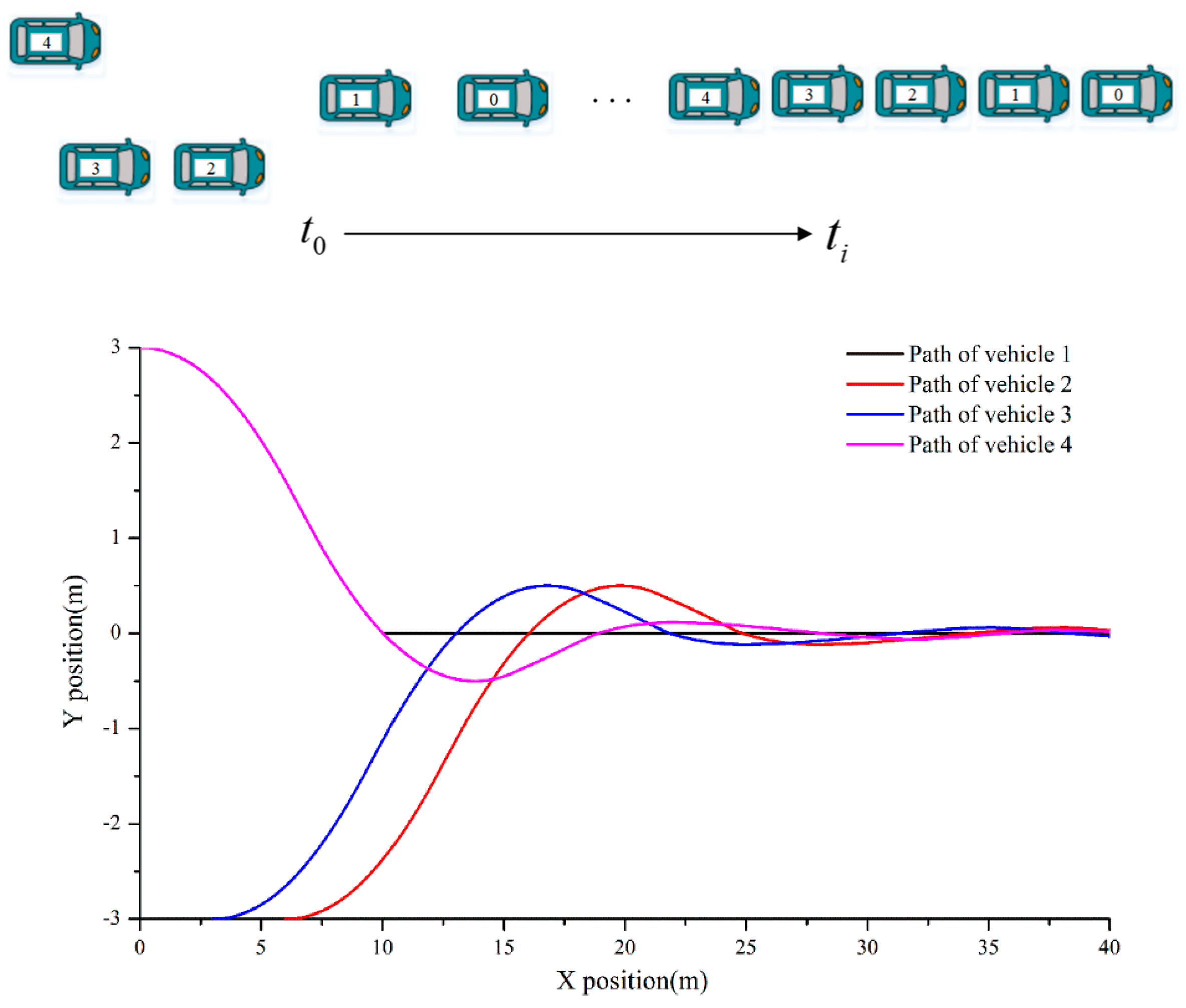
The platoon can be applied in the direction of commercial vehicles for medium and long-distance cargo transportation and common individual vehicles seeking collaborators to save fuel and reduce driver workload. When there are enough vehicles gathered for the same or similar purposes and ready for coordinated control, each vehicle needs to form the geometry that is required by the platoon. When the market share of cars with multi-vehicle coordination ability is low, the ratio of intelligent cooperative vehicles in a local area can be increased by this way, so that the advantages of queue coordination control become more obvious [25]. The aggregation of the platoon requires that, when the leading vehicle issues a platoon merging command, the potential following vehicle can arrive at a regular lane or a dedicated lane according to a particular order, and there is no additional acceleration, braking, or lane change in the process.
It is assumed that both the leading vehicle and the following vehicle have communication capabilities so that the balanced point of the leading vehicle setting can be known. To strike a balanced between accuracy and conciseness, it is assumed that: constant spacing control strategy is used in control, which means that the distance between the desired balanced point of the following vehicle and the leading vehicle is constant. In the platoon merging, different FWIDSVs in different positions determine their own balanced points under the coordination of the pilot vehicles, and coordinate and merge. The position and spacing information of the pilot vehicle and the FWIDSV as the following vehicle are shown in the Table 4.
Through the Figure 15, it can be seen that FWIDSVs located at different initial positions track the path and stabilize at their own balanced point after obtaining the coordinated command of the leading vehicle. The following vehicles at different locations can operate normally, which shows that the controller has good control performance under a longitudinal and lateral coupling situation.
5. Conclusions
In this paper, we investigated a FWIDSV vehicle platoon coordination and path tracking control method based on the RVF. When compared to other platoon coordination control systems, MPC has a complex calculation process and poor real-time computing ability; the PID controller is difficult to handle longitudinal and lateral coupling motion problem. The desired acceleration of following vehicle could be obtained via RVF to track the reference path and follow the leading vehicle simultaneously. It is a kind of coupling control system that can make full use of tire forces, hence it is more suitable for FWIDSV. Through the simulation validations and result analysis, some conclusions are briefly discussed here:
- Through simulation in ICC scenarios, the proposed control method shows great performance, indicating that a reasonable RVF has good applicability in the ICC scenarios. It can be found that the tire force is effectively distributed, so that the path tracking and spacing maintaining are conducted simultaneously. The error can be effectively converged by RVF.
- The desired acceleration from the RVF is achieved by constructing the FWIDSV integrated controller. The LQP-based tire force distribution method and the linerazing constraint avoid the problem of actuator saturation, thus ensuring the safety and stability of FWIDSV. It should be pointed out that there are reasonable errors between the desired accelerations obtained from following control layer and the actual accelerations of FWIDSV, which result form the hysteresis, non-linearity, and motion resistance of the execution system.
- In the platoon merging scenario, the following FWIDSVs are brought together in a line from different initial points, which means that FWIDSV platoon coordination and the tracking method based on RVF demonstrate great application potential, and can realize complex and practical driving tasks.
Our findings suggest that the use of RVF might provide a viable potential for cooperative platoon control in the future. In the construction of the RVF, to maintain the distance between the following vehicle and the leading vehicle in the longitudinal direction, the norm of the flow vector is set to be related to the speed of the leading vehicle and the longitudinal tracking error. The selection of the gain coefficient k has a particular impact on the tracking effect, even conflicting in the longitudinal and lateral directions. Therefore, the main parameters of the RVF can be optimized with specific optimization objectives, to obtain the optimal control effect in the further studies. Besides, a constant longitudinal spacing control strategy is adopted, provided that the distance between the balanced point and the leading vehicle is fixed. In the platoon merging scenario, it assumes that the safety and traffic rules have been taken into account when the leading vehicle coordinates the number of the following vehicles; thus, interaction between the following vehicles is weakened. Under the control of the RVF, the collision avoidance condition can also be discovered in the future, which has great significance for vehicle platoon control.
Author Contributions
Conceptualization, data curation, writing—original draft preparation, Y.L.; review and editing, C.Z.; formal analysis, T.J.G.; software and data analysis, G.L.; methodology providing, D.Z.
Funding
This research is funded by scientific study project for institutes of higher learning of Liaoning Provincial Department of Education (JP2016018).
Acknowledgments
In this section you can acknowledge any support given which is not covered by the author contribution or funding sections. This may include administrative and technical support, or donations in kind (e.g., materials used for experiments).
Conflicts of Interest
The authors declare no conflict of interest.
References
- Shladover, S.E.; Nowakowski, C.; Lu, X.Y.; Ferlis, R. Cooperative adaptive cruise control definitions and operating concepts. Transp. Res. Rec. J. Transp. Res. Board 2015, 2489, 145–152. [Google Scholar] [CrossRef]
- Gao, F.; Li, S.E.; Zheng, Y.; Kum, D. Robust control of heterogeneous vehicular platoon with uncertain dynamics and communication delay. IET Intell. Transp. Syst. 2016, 10, 503–513. [Google Scholar] [CrossRef]
- Liu, H.; Kan, X.; Shladover, S.E.; Lu, X.Y.; Ferlis, R.E. Impact of cooperative adaptive cruise control on multilane freeway merge capacity. J. Intell. Transp. Syst. 2018, 22, 263–275. [Google Scholar] [CrossRef]
- Arnaout, G.M.; Arnaout, J.P. Exploring the effects of cooperative adaptive cruise control on highway traffic flow using microscopic traffic simulation. Transp. Plan. Technol. 2014, 37, 186–199. [Google Scholar] [CrossRef]
- Khatir, M.E.; Davison, E.J. A decentralized lateral-longitudinal controller for a platoon of vehicles operating on a plane. In Proceedings of the 2006 American Control Conference, Minneapolis, MN, USA, 14–16 June 2006; pp. 5891–5896. [Google Scholar] [CrossRef]
- Englund, C.; Chen, L.; Ploeg, J.; Semsar-Kazerooni, E.; Voronov, A.; Bengtsson, H.H.; Didoff, J. The grand cooperative driving challenge 2016: Boosting the introduction of cooperative automated vehicle. IEEE Wirel. Commun. 2016, 23, 146–152. [Google Scholar] [CrossRef]
- Chang, C.; Yuan, Z. Combined longitudinal and lateral control of vehicle platoons. In Proceedings of the 2017 International Conference on Computer Systems, Electronics and Control, Dalian, China, 25–27 December 2017; pp. 848–853. [Google Scholar]
- Fujioka, T.; Suzuki, K. Control of longitudinal and lateral platoon using sliding control. Veh. Syst. Dyn. 1994, 23, 647–664. [Google Scholar] [CrossRef]
- Rajamani, R.; Tan, H.S.; Law, B.K.; Zhang, W.B. Demonstration of integrated longitudinal and lateral control for the operation of automated vehicles in platoons. IEEE Trans. Control Syst. Technol. 2000, 8, 695–708. [Google Scholar] [CrossRef]
- Shuai, Z.; Zhang, H.; Wang, J.; Li, J.; Ouyang, M. Lateral motion control for four-wheel-independent-drive electric vehicles using optimal torque allocation and dynamic message priority scheduling. Control Eng. Pract. 2014, 24, 55–66. [Google Scholar] [CrossRef]
- Huang, B.; Wu, S.; Huang, S.; Fu, X. Lateral stability control of four-wheel independent drive electric vehicles based on model predictive control. Math. Probl. Eng. 2018, 2018, 6080763. [Google Scholar] [CrossRef]
- Guo, J.; Luo, Y.; Li, K. An adaptive hierarchical trajectory Following control approach of autonomous four-wheel independent drive electric vehicles. IEEE Trans. Intell. Transp. Syst. 2018, 19, 2482–2492. [Google Scholar] [CrossRef]
- Gordon, T.J.; Best, M.C.; Dixon, P.J. An automated driver based on convergent vector fields. Proc. Inst. Mech. Eng. Part D J. Automob. Eng. 2002, 216, 329–347. [Google Scholar] [CrossRef] [Green Version]
- Pamosoaji, A.K.; Hong, K.S. A path-planning algorithm using vector potential functions in triangular regions. IEEE Trans. Syst. Man Cybern. Syst. 2013, 43, 832–842. [Google Scholar] [CrossRef]
- Matveev, A.S.; Hoy, M.C.; Savkin, A.V. Extremum seeking navigation without derivative estimation of a mobile robot in a dynamic environmental field. IEEE Trans. Control Syst. Technol. 2016, 24, 1084–1091. [Google Scholar] [CrossRef]
- Hoy, M.; Matveev, A.S.; Savkin, A.V. Algorithms for collision-free navigation of mobile robots in complex cluttered environments: A survey. Robotica 2015, 33, 463–497. [Google Scholar] [CrossRef]
- Jansen, W. Lateral Path-Following Control for Automated Vehicle Platoons. Master’s Thesis, Delft University of Technology, Delft, The Netherlands, 2016. [Google Scholar]
- Feng, Y.; Yu, X.; Man, Z. Non-singular terminal sliding mode conrol of rigid maniplators. Automatica 2002, 38, 2159–2167. [Google Scholar] [CrossRef]
- Song, P.; Tomizuka, M.; Zong, C. A novel integrated chassis controller for full drive-by-wire vehicles. Veh. Syst. Dyn. 2015, 53, 215–236. [Google Scholar] [CrossRef]
- Sakai, S.; Sado, H.; Hori, Y. Dynamic Driving/Braking Force Distribution in Electric Vehicle with Independently Driven Four Wheels. Electr. Eng. Jpn. 2000, 138, 79–89. [Google Scholar] [CrossRef]
- Li, B.; Du, H.; Li, W. A protential field approach-based trajectory control for autonomous electric vehicles with in-wheel motors. IEEE Trans. Intell. Transp. Syst. 2017, 18, 2044–2055. [Google Scholar] [CrossRef]
- Jiang, K. Real-Time Estimation and Diagnosis of Vehicle’s Dynamics States with Low-Cost Sensors in Different Driving Condition. Ph.D. Thesis, Federal University of Minas Gerais, Belo Horizont, Brazil, 2016. [Google Scholar]
- Chen, T.; Xu, X.; Chen, L.; Jiang, H.; Cai, Y.; Li, Y. Estimation of longitudinal force, lateral vehicle speed and yaw rate for four-wheel independent driven electric vehicles. Mech. Syst. Signal Process. 2018, 101, 377–388. [Google Scholar] [CrossRef]
- Mashadi, B.; Mahmoodi-K, M.; Kakaee, A.H.; Hosseini, R. Vehicle plath following control in the presence of driver inputs. J. Multi-Body Dyn. 2014, 227, 115–132. [Google Scholar] [CrossRef]
- Olia, A.; Razavi, S.; Abdulhai, B.; Abdelgawad, H. Traffic capacity implications of automated vehicles mixed with regular vehicles. J. Intell. Transp. Syst. 2017, 22, 244–262. [Google Scholar] [CrossRef]
Figure 1.
Platoon path following strategy. Vehicle 0 denotes the leading vehicle. Other vehicles denote the following vehicles in platoon.
Figure 1.
Platoon path following strategy. Vehicle 0 denotes the leading vehicle. Other vehicles denote the following vehicles in platoon.

Figure 2.
The diagram of reference vector.
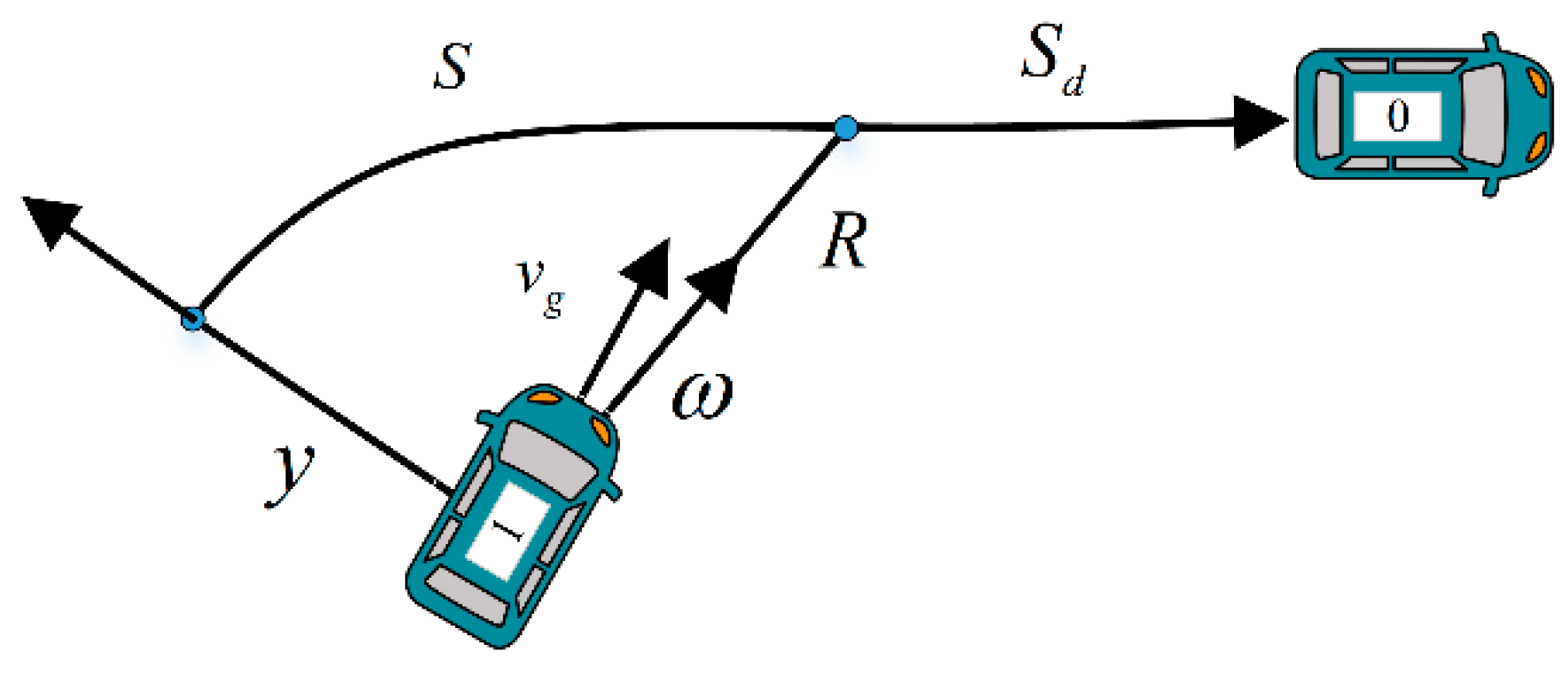
Figure 3.
Control variables in friction circle.
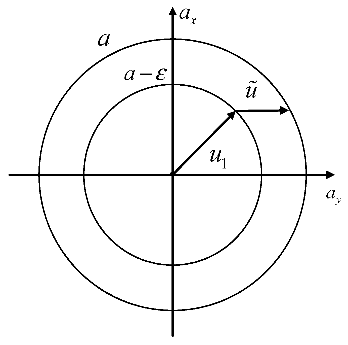
Figure 4.
Particle motion under the different values of ε: (a) The path of particle model in the global coordinate system under the different values of ε; and, (b) The longitudinal following error of particle model under the different values of ε.
Figure 4.
Particle motion under the different values of ε: (a) The path of particle model in the global coordinate system under the different values of ε; and, (b) The longitudinal following error of particle model under the different values of ε.
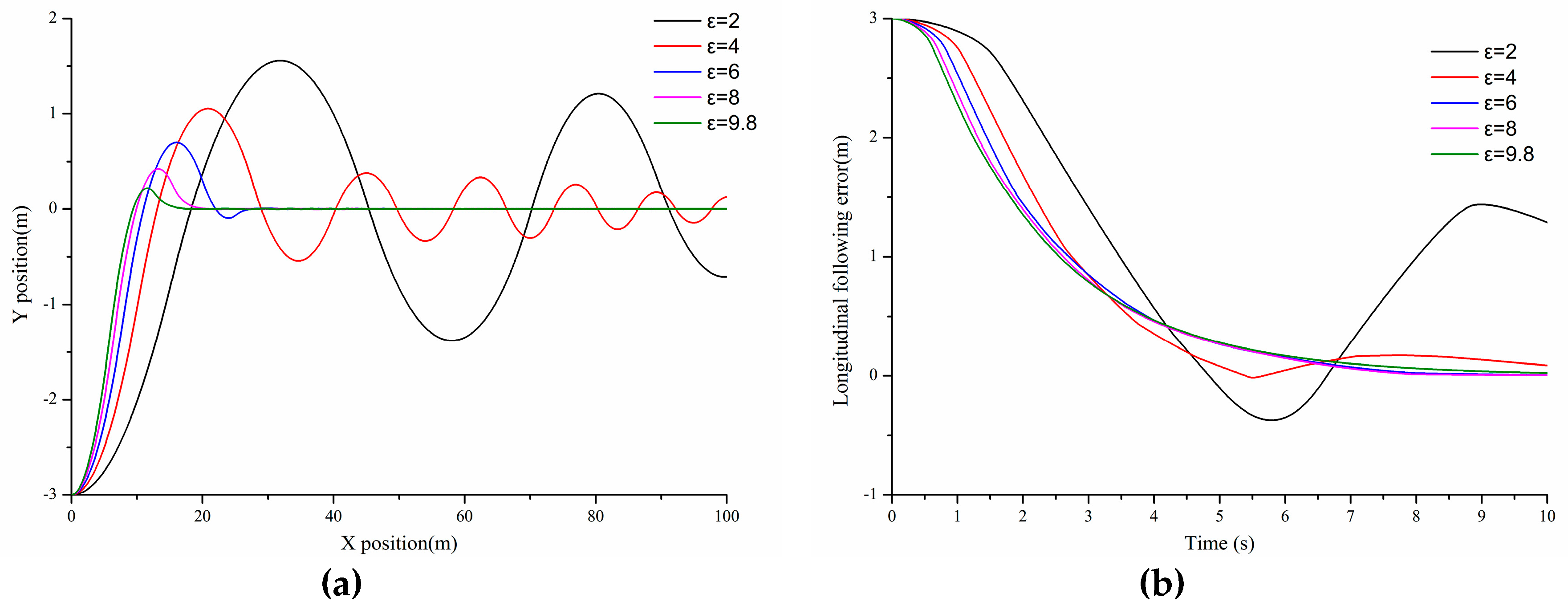
Figure 5.
Particle motion under the different values of k: (a) The path of particle model under the different values of k; and, (b) The following error of particle model under the different values of k.
Figure 5.
Particle motion under the different values of k: (a) The path of particle model under the different values of k; and, (b) The following error of particle model under the different values of k.
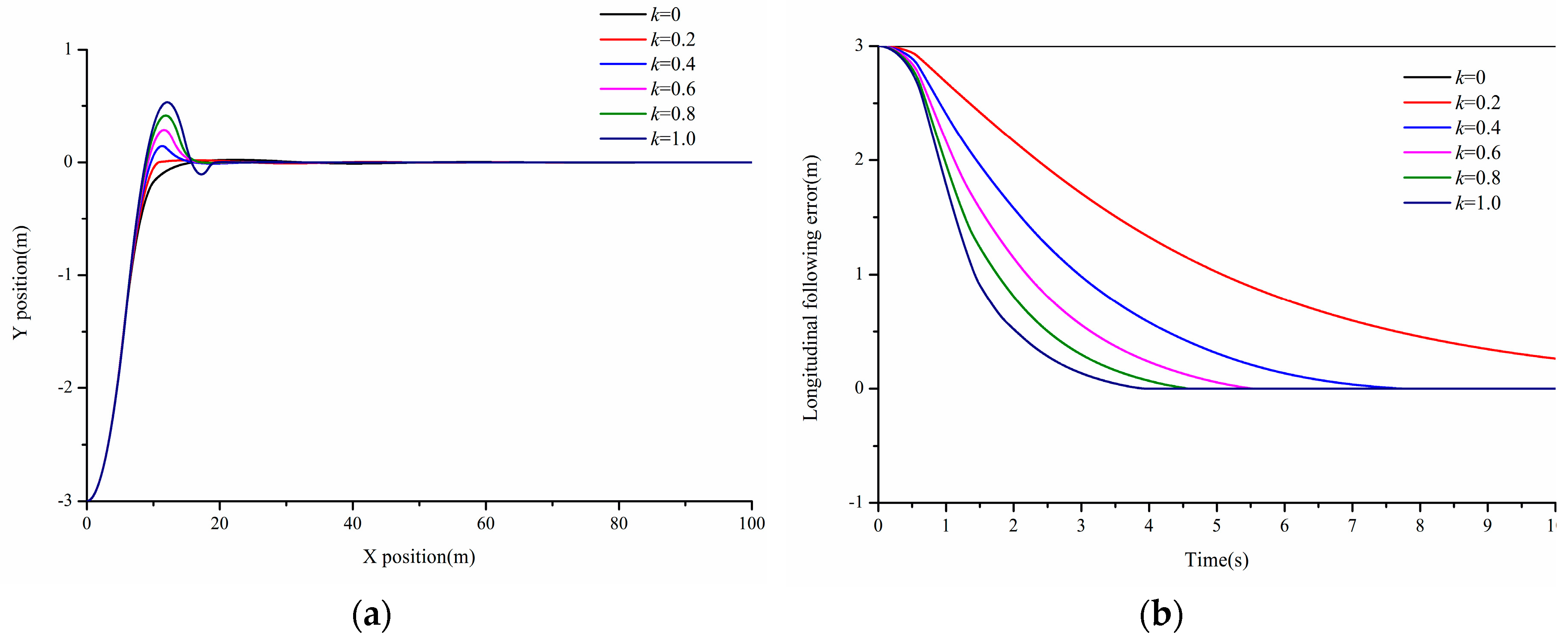
Figure 6.
Effect of the tracking error convergence.
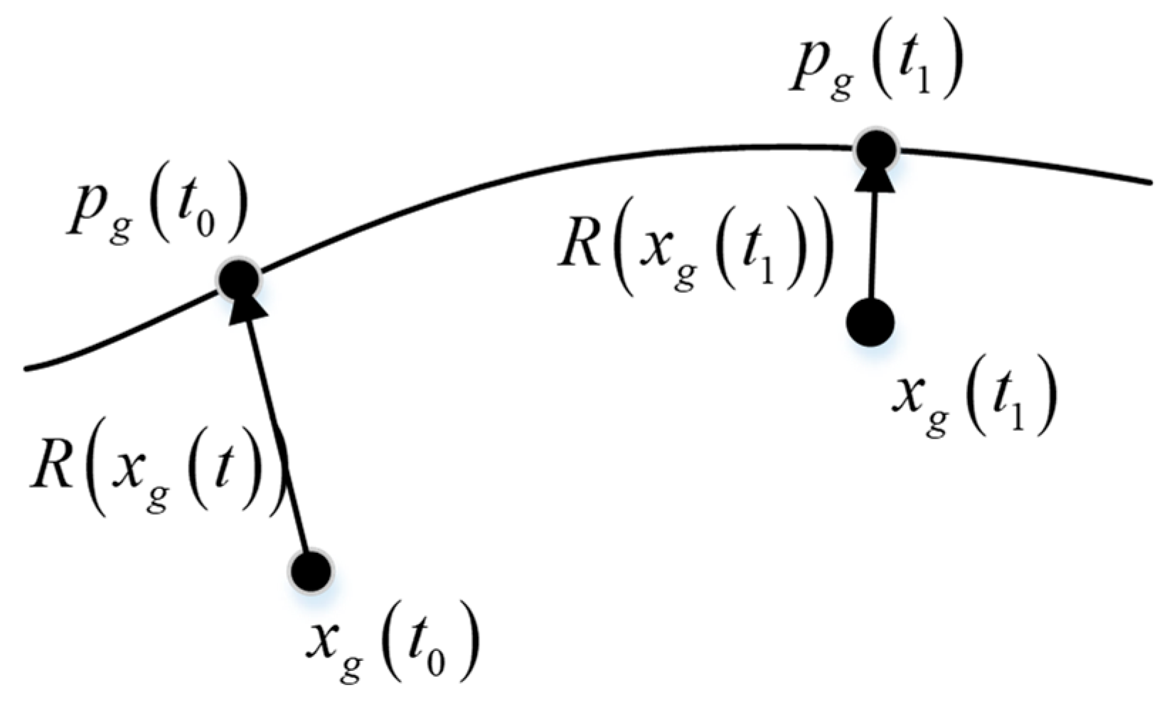
Figure 7.
Structure of four-wheel independent driving and steering (FWIDSV) platoon following control.
Figure 7.
Structure of four-wheel independent driving and steering (FWIDSV) platoon following control.
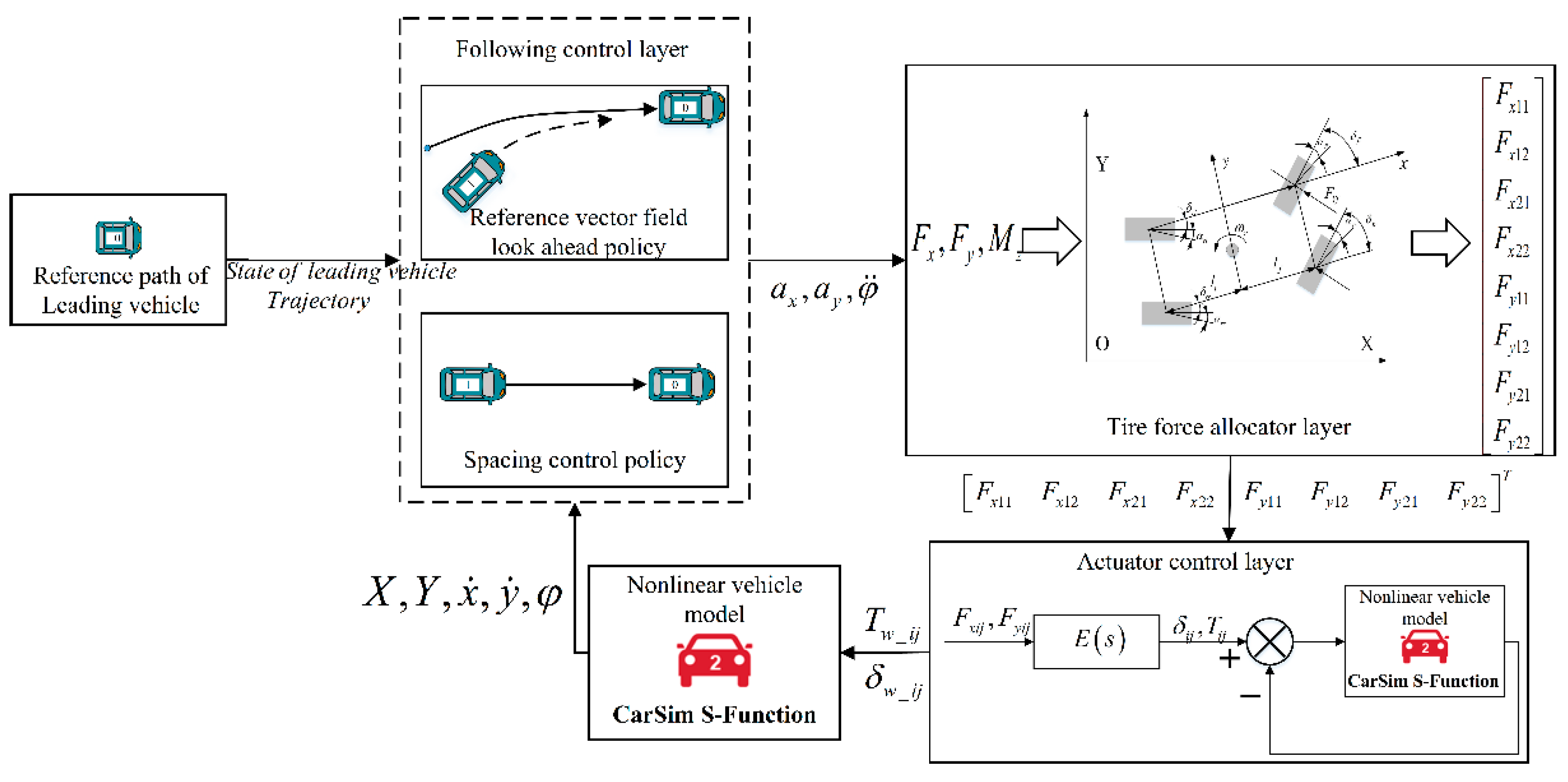
Figure 8.
The schematic of FWIDSV.
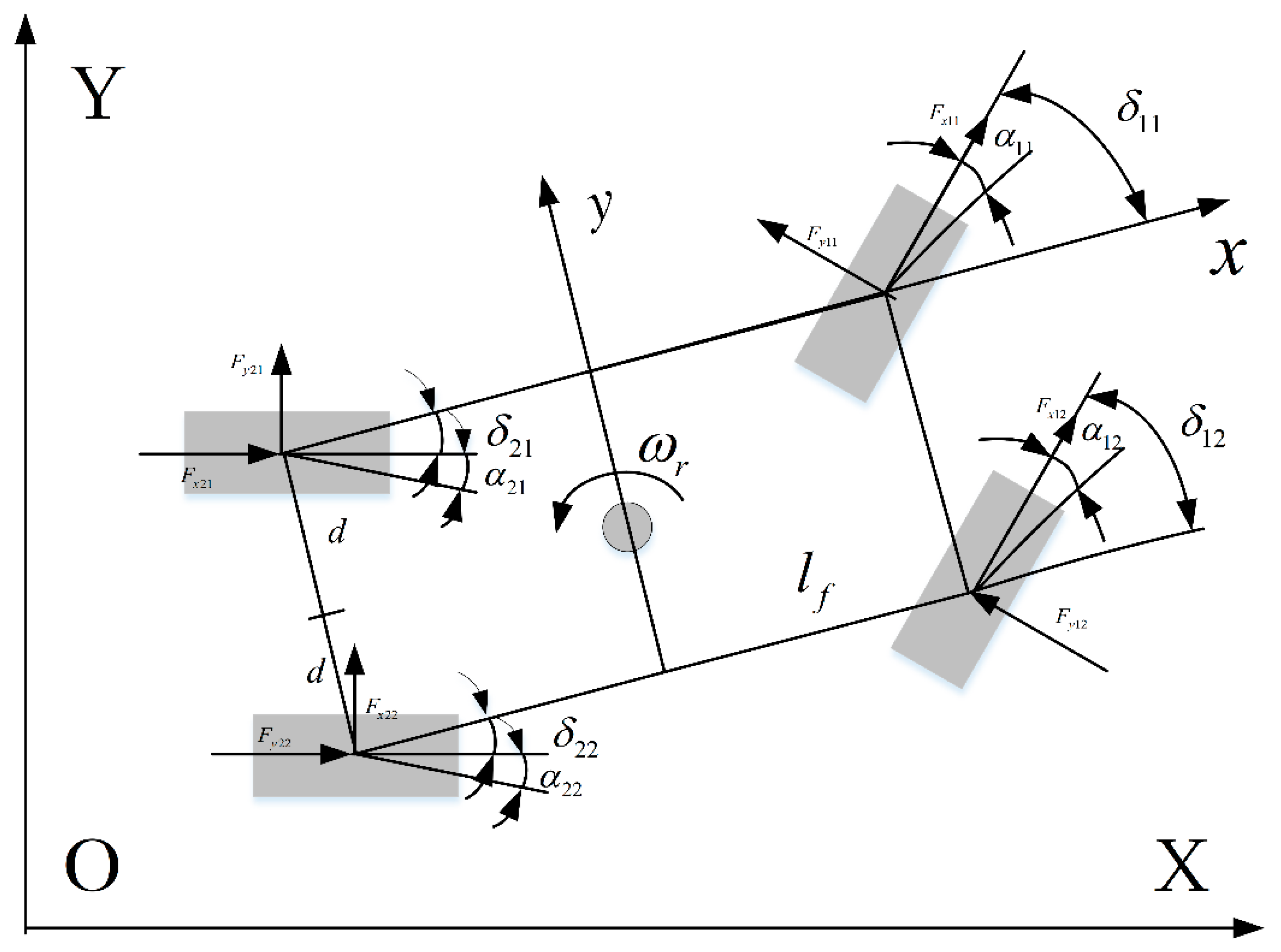
Figure 9.
The schematic of linear polygon constraint.
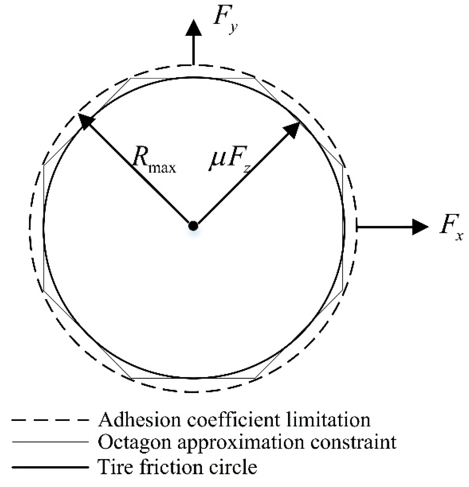
Figure 10.
Structure of actuator control layer.

Figure 11.
Motion of different model: (a) The path comparison of different models; and, (b) The following error comparison of different models.
Figure 11.
Motion of different model: (a) The path comparison of different models; and, (b) The following error comparison of different models.
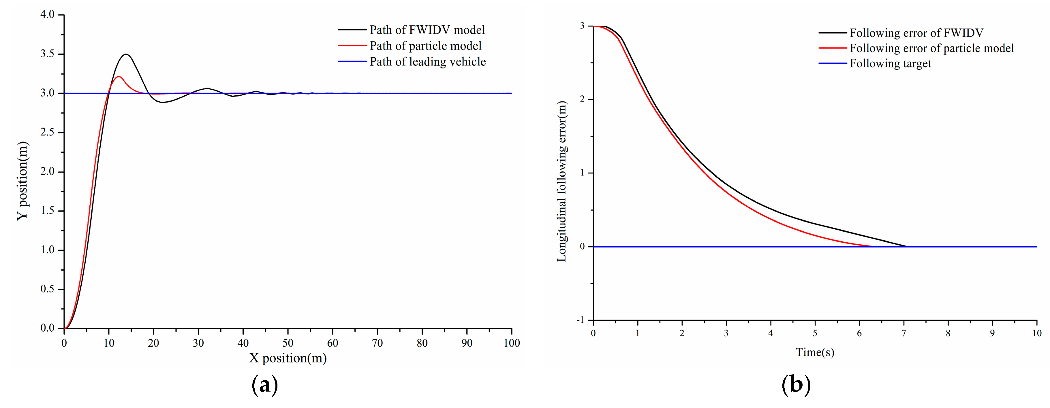
Figure 12.
The usage of tire force and acceleration curve: (a) The usage of friction circle; and, (b) The comparison between desire acceleration and actual acceleration.
Figure 12.
The usage of tire force and acceleration curve: (a) The usage of friction circle; and, (b) The comparison between desire acceleration and actual acceleration.

Figure 13.
Curves of driving torques and steering angles of FWIDSV: (a) The curves of driving torque; and, (b) The curves of steering angles.
Figure 13.
Curves of driving torques and steering angles of FWIDSV: (a) The curves of driving torque; and, (b) The curves of steering angles.

Figure 14.
Tracking performance in curved road: (a) The path of the vehicles; and, (b) The longitudinal following error.
Figure 14.
Tracking performance in curved road: (a) The path of the vehicles; and, (b) The longitudinal following error.
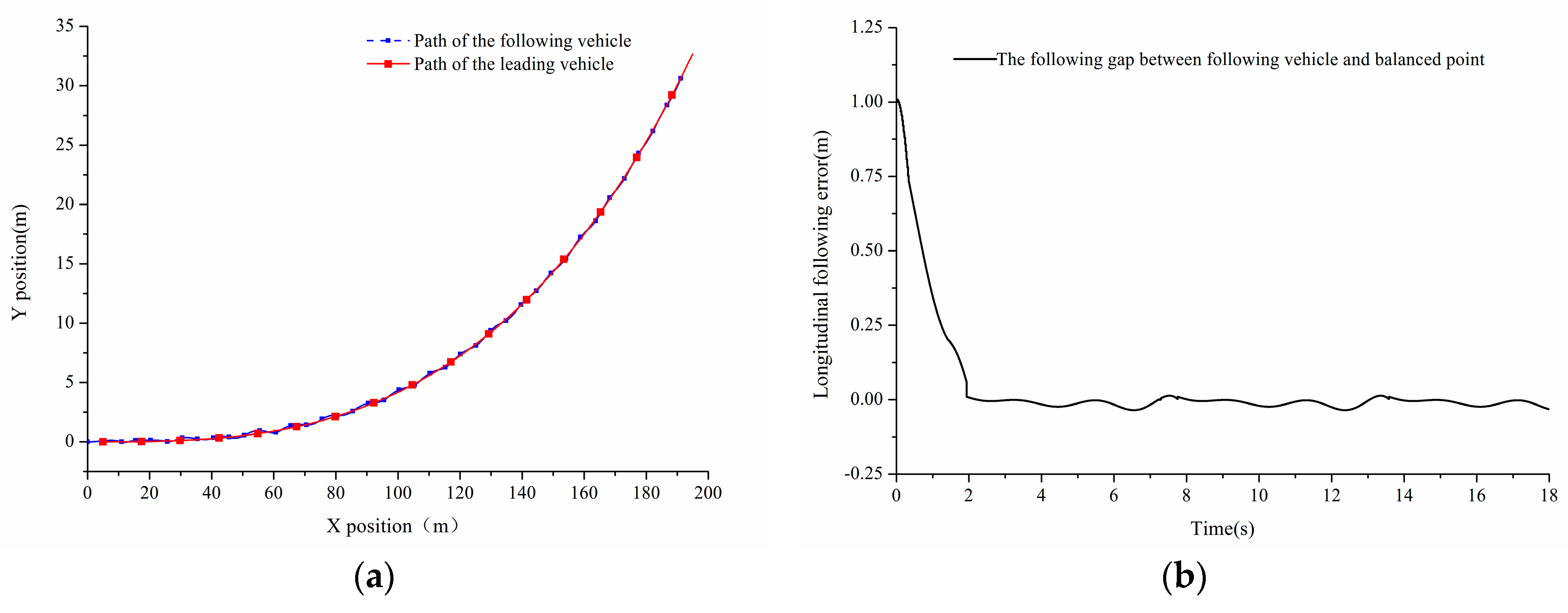
Figure 15.
Vehicle path in platoon merging.

Table 1.
Parameters of controller.
| Symbols | Value |
|---|---|
| α | 0.072 |
| β | 1 |
| q | 13 |
| p | 15 |
Table 2.
The meaning of the symbols.
| Symbols | Meaning | Symbols | Meaning |
|---|---|---|---|
| δij | Steering angles of roadwheels | ayd | Desired lateral acceleration in vehicle coordinate system |
| αij | Tire side angles | Yaw angle acceleration | |
| Longitudinal speed of vehicle | m | Mass | |
| Lateral speed of vehicle | l1 | Front wheelbase | |
| φ | Yaw of the vehicle | l2 | Rear wheelbase |
| Yaw rate of the vehicle | d | Half of the tread | |
| F | The tire forces | μ | Ground adhesion coefficient |
| axd | Desired longitudinal acceleration in vehicle coordinate system | Iz | Yaw inertia |
Table 3.
Vehicle parameters.
| Symbols | Descriptions | Values |
|---|---|---|
| M(kg) | Total mass of vehicle | 1020 |
| Iz(kg∙m2) | Moment of inertia around vertical axis | 1020 |
| lf(m) | Front wheelbase | 1.165 |
| lr(m) | Rear wheelbase | 1.165 |
| d(m) | Half of the wheel tread | 0.875 |
Table 4.
Vehicle parameters.
| Vehicle ID | Classification | Initial Position | The Pre-set Desired Inter-Vehicular Spacing |
|---|---|---|---|
| 0 | Leading vehicle | 15, 0 | \ |
| 1 | Following vehicle | 10, 0 | 3 |
| 2 | Following vehicle | 6, −3 | 3 |
| 3 | Following vehicle | 3, −3 | 3 |
| 4 | Following vehicle | 0, 3 | 3 |
© 2019 by the authors. Licensee MDPI, Basel, Switzerland. This article is an open access article distributed under the terms and conditions of the Creative Commons Attribution (CC BY) license (http://creativecommons.org/licenses/by/4.0/).
Share and Cite
MDPI and ACS Style
Liu, Y.; Zhang, D.; Gordon, T.; Li, G.; Zong, C. Approach of Coordinated Control Method for Over-Actuated Vehicle Platoon based on Reference Vector Field. Appl. Sci. 2019, 9, 297. https://doi.org/10.3390/app9020297
AMA Style
Liu Y, Zhang D, Gordon T, Li G, Zong C. Approach of Coordinated Control Method for Over-Actuated Vehicle Platoon based on Reference Vector Field. Applied Sciences. 2019; 9(2):297. https://doi.org/10.3390/app9020297
Chicago/Turabian StyleLiu, Yang, Dong Zhang, Timothy Gordon, Guiyuan Li, and Changfu Zong. 2019. "Approach of Coordinated Control Method for Over-Actuated Vehicle Platoon based on Reference Vector Field" Applied Sciences 9, no. 2: 297. https://doi.org/10.3390/app9020297
Note that from the first issue of 2016, this journal uses article numbers instead of page numbers. See further details here.