Model-Free Identification of Nonlinear Restoring Force with Modified Observation Equation


1
College of Civil Engineering, Hunan University, Changsha 410082, China
2
Key Laboratory of Building Safety and Energy Efficiency, Ministry of Education, Changsha 410082, China
3
College of Civil Engineering, Huaqiao University, Xiamen 361021, China
*
Author to whom correspondence should be addressed.
Appl. Sci. 2019, 9(2), 306; https://doi.org/10.3390/app9020306
Submission received: 12 December 2018
/
Revised: 29 December 2018
/
Accepted: 11 January 2019
/
Published: 16 January 2019
(This article belongs to the Special Issue Structural Damage Detection and Health Monitoring)
Abstract
:Nonlinearity exists widely in civil engineering structures; for example, the initiation and growth of damage under dynamic loadings is a typical nonlinear process. To date, for the purpose of structural evaluation and a better understanding nonlinear characteristics of complicated structures, a number of parametric and nonparametric methods have been developed for the identification of nonlinear restoring force (NRF). However, due to the highly individualistic nature of nonlinear systems, it would be inefficient to attempt to express the structural NRF in a general parametric form. For many nonparametric techniques, their nonparametric models or approximations may result in undesirable results or oscillations around unsmooth points. In this paper, on the basis of extended Kalman filter (EKF), a model-free NRF identification approach is proposed to circumvent the limitations mentioned above. The NRF to be identified was treated as ‘unknown fictitious input’, and thus, no prior assumptions or approximations for the NRF model were required. With the aid of a projection matrix, a modified version of observation equation was obtained. Based on the principle of EKF, the recursive solution of the proposed approach was analytically derived. The NRFs provided by the nonlinear components were identified by means of least squares estimation (LSE) at each time step. Numerical examples, including building structures equipped with magnetorheological (MR) damper and shape memory alloy (SMA) damper, demonstrated that the proposed approach is capable of satisfactorily identifying NRF without knowledge or intuitive assumptions of any nonlinear model class in advance.
1. Introduction
1.1. Background
Civil engineering structures are prone to deterioration or damage due to certain factors, such as strong dynamic loadings, material fatigue accumulation and environmental corrosion. To date, a variety of vibration-based damage detection and system identification methods have been developed [1,2]. Most of them are applicable when the structure of interest is linear. However, nonlinearity is generic in nature, and linear behavior is an exception [3]. The occurrence of a fault in an initially linear structure will, in many cases, result in nonlinear behavior. Therefore, it is highly desirable to develop nonlinear identification algorithms to facilitate the evaluation of the structural performance and condition for the purpose of prevention of potentially catastrophic events.
It is known that typical sources of nonlinearities include geometric nonlinearity, inertia nonlinearity, material nonlinearity and boundary nonlinearity. It is of importance to have an accurate model for the description of the nonlinear behavior of the physical structure prior to parameter estimation. Nonlinear modeling is a challenging step, because nonlinearity may be caused by many different mechanisms and may result in plethora of dynamic phenomena. Without a precise understanding of the nonlinear mechanisms involved, the identification process is bound to fail. A priori knowledge and nonlinearity classification may help to select a reasonably accurate model of the nonlinearity. If little is known about the form of the model before starting the identification process, one may resort to nonparametric approximations or expressions.
1.2. Literature Survey
Since the restoring force can act as an indicator of the extent of the nonlinearity and be used to quantitatively evaluate the absorbed energy during vibration, the research on nonlinear restoring force (NRF) identification has been actively conducted over years and the comprehensive literature reviews can be found [3,4]. Broadly speaking, the existing NRF identification methods can be divided into two groups, i.e., parametric identification and nonparametric identification. In parametric identification methods, a model structure is specified, whereas the primary quantities obtained from the nonparametric identification methods do not directly specify equations of motion [5]. Once the structural model is fixed, the nonlinear identification problem is reduced to parameter estimation as only the coefficients of the model terms remain unspecified. The subject of parametric nonlinear identification is extremely broad, and an extensive literature exists (e.g., [6,7,8,9,10]). It is not intended to provide a comprehensive overview of the past and current approaches for the parametric identification of nonlinearity in this paper. Instead, some relevant research regarding extended Kalman filter (EKF)-based nonlinear parameter identification methods is introduced herein. For example, Yang et al. [11] proposed an EKF-based adaptive tracking technique for the identification of time-vary parameters of linear and nonlinear hysteretic structures. The performance of EKF and Unscented Kalman filter (UKF) for the nonlinear identification was discussed in details by Wu and Smyth [12]. Based on the sequential application of extended Kalman estimator and least squares estimation (LSE), Lei et al. [13] proposed an algorithm for the identification of nonlinear structural parameters. On the basis of the orthogonal decomposition of excitation, Ding et al. [14] proposed an EKF-based method for the condition assessment of linear and nonlinear hysteretic structures. By using EKF to estimate time-invariant parameters of the nonlinear material constitutive models, a novel nonlinear finite element model updating framework was proposed by Ebrahimian et al. [15]. A two-stage NRF identification method was proposed by Lei et al. [16] by using EKF for the determination of nonlinear locations in the first stage and the estimation of NRFs in the second stage. This method was extended by Liu et al. [17] for identifying strong nonlinearity parameters. With the combination of EKF and dynamic statistical process control, Jin et al. [18] presented a novel real-time damage detection method for identifying the parameters of both linear and nonlinear structures under different damage scenarios. Xiao et al. [19] proposed an adaptive three-stage EKF method to solve state and fault estimation in nonlinear discrete-time system. A dual adaptive filtering approach was proposed by Astroza [20] for nonlinear finite element model updating with the consideration of modeling uncertainty. The performance of different model updating techniques using EKF, UKF and iterated EKF were further compared by Astroza et al. [21] in terms of convergence, accuracy, robustness and computational demand.
The methods mentioned above are all capable of identifying the NRF of a preset nonlinear model. However, accessing prior knowledge of nonlinear characteristics may prove difficult in many circumstances owing to the highly individualistic nature of real nonlinearities. Moreover, it is sometimes difficult to define a specific physically-motivated model to precisely describe the encountered nonlinear phenomena such as the initiation and development of crack. The lack of high-fidelity, physics-based and robust models that could accurately reflect the multidimensional behavior of these nonlinear systems would hinder the application of the computational tools or methods in identifying the complex nonlinearities in the design stage. Thus, nonparametric nonlinear identification solely using input and output data is necessary. Increasing attention has been received in this area and much progress has been made. Early contributions to nonparametric nonlinear identification can be traced back to the 1980s when Masri et al. developed their famous restoring force surface (RFS) methods by using Chebyshev polynomial [22,23,24,25]. The data processing and experimental design for the investigation of RFS method were further conducted by Worden [26,27]. A two-stage general procedure was presented by Masri et al. [28] for developing data-based, model-free representations of complex nonlinear systems under arbitrary dynamic loads. By using a power series polynomial to represent the NRF, a data-based approach was proposed for the identification of chain-like structure equipped with magneto-rheological (MR) damper [29,30] and shape memory alloy (SMA) damper [31]. The generalized two-variable Chebyshev polynomials and their relevant relations were further discussed by Cesarano and Fornaro [32,33]. A data-based nonlinear identification approach was proposed by Xu et al. [34] for mass and NRF identification under incomplete loadings. By introducing an equivalent linear structural system and a power series polynomial, Lei et al. [35] proposed an EKF-based model-free NRF identification approach for the identification of the unknown coefficients of the power series polynomials and other structural parameters. Su et al. [36] proposed a two-step approach to identify the nonlinearities of model-free MR damper with partial response data. Based on the Hilbert transform, two novel nonparametric identification approaches were proposed by Yuan et al. [37] for nonlinear piezoelectric mechanical systems. Ondra et al. [38] proposed a zero-crossing method for nonparametric identification of systems with asymmetric NRFs. As the rapid development of computers and their associated computational capabilities, the intelligent black-box methods for nonparametric nonlinear identification using artificial neural networks, fuzzy networks, genetic algorithms and so forth have received increasing attention. The literature review on these natural computing methods with different emphasis can be found [4,39].
1.3. Scope
Most of the aforementioned nonparametric identification methods are based on the usage of some specific nonparametric expressions to describe or approximate the nonlinear properties. The key of these methods is to properly determine the values of the coefficients in their nonparametric expressions basing on the input and output data. Such approximations may, however, result in undesirable oscillations or inaccurate results around unsmooth points. In this paper, an EKF-based model-free nonlinear identification approach is proposed for the identification of NRFs and other structural parameters. By using a projection matrix, a modified version of observation equation is obtained. The NRF is treated as ‘unknown fictitious input’ and identified by means of LSE. Based on the principle of EKF, the recursive solution of the proposed approach is analytically derived. The proposed approach requires input and output data only, without knowledge or intuitive assumptions of any nonlinear model class in advance.
The present research work is organized as follows: Section 2: formulation of the proposed model-free NRF identification procedure; Section 3: validation of the proposed approach via a building structure equipped with MR damper and SMA damper; Section 4: conclusions and discussions of the proposed approach.
2. Formulas of the Proposed Approach
The general equation of motion of a discrete n-DOFs nonlinear structure under external excitations can be expressed as:
in which M is the mass matrix and assumed to be known; C and K are the damping matrix and stiffness matrix, respectively; and x(t) are acceleration, velocity and displacement responses, respectively; is the vector of NRF; f(t) is the external excitation and assumed to be available in this study; ηu and φ are the influence matrix associated with and f(t), respectively.
Here, the state vector of the structure is defined as , where θ is the unknown time-invariant structural parameters (i.e., stiffness and damping coefficients). Then, the following state equation can be found:
where w(t) is model noise vector with zero mean and a covariance matrix .
It should be noted, besides the unknown structural parameters, the NRF is assumed to be unavailable as well. Since the NRF is treated as ‘unknown fictitious inputs’ herein, it can be found the prior knowledge or intuitive assumptions of any nonlinear model class of NRF is not required. Let and be the estimations of and , respectively. Using Taylor expansion, Equation (2) can be linearized at time instant t = k × ∆t with the sampling interval of ∆t:
where the subscript k denotes the k-th time step:
In consideration of , one can obtain the following expression with the aid of Equations (2) and (3):
Generally, the acceleration responses are more easily obtained and reliable as compared with other responses, such as displacement and velocity. Thus, the acceleration is assumed to be measured in this study. The discretized observation equation can be then expressed as:
where yk is the measured acceleration vector; the subscript k denotes time step t = k × ∆t; vk is the measurement noise vector assumed to be a Gaussian white noise vector with zero mean and a covariance matrix Equation (6) can be also re-written as:
where ; .
The re-arrangement of Equation (7) leads to the following expression:
The closest solution of can be then obtained using LSE as:
The error of the aforementioned solution can be calculated as:
where I is an identity matrix; is known as the projection matrix. As a limit, the error shown in Equation (10) should tend to be zero, leading to:
in which . As compared with Equation (6), it can be found that multiple unknown issues have been transformed into a single unknown problem. Then, the EKF technique can be used to deal with such single regression problem.
Analogous to the traditional EKF, the priori state estimate can be given as:
Then, with the combination of Equation (5), the priori estimate error can be found as:
Focusing on the second term on the right-hand-side of Equation (13), the following transformation can be obtained:
Similarly, can be linearized as follows:
where:
Substituting Equations (14) and (15) into Equation (13) leads to:
where:
The priori estimate error covariance matrix can be then determined as:
Based on Equation (11) and the principle of KF, the posteriori state estimate herein can be calculated as a linear combination of the priori state estimate and a weighted difference between the actual measurements and the corresponding predictions:
where Gk+1 is the gain matrix at time step t = (k + 1) × Δt. Based on Equations (5), (15) and (20), the posteriori estimate error can be calculated as:
where Hk+1|k can be determined using Equation (16) when .
Accordingly, the posteriori estimate error covariance matrix can be obtained as:
Based on the principle of EKF, the gain matrix can be determined by the following equation:
where tr(·) denotes the trace operator. Then, one can obtain:
Once the posteriori state estimate is determined through Equation (20), the unknown NRF can be determined by Equation (9) as follows:
It is clear that the recursive solution for the proposed approach includes priori estimation through Equations (12) and (19), posteriori estimation through Equations (20) and (22), gain matrix calculation by Equation (24), as well as NRF identification by Equation (25). The effectiveness and robustness of the proposed method will be verified via several numerical examples in the following section.
3. Numerical Application
Here, a six-story shear building structure equipped with different types of nonlinear hysteretic dampers was used to demonstrate the effectiveness of the proposed approach. The parameters of the building structure were assumed to be mi = 300 kg and ki = 1.8 × 10⁵ N/m (i = 1, 2, …, 6). The Rayleigh damping assumption was adopted with the proportional coefficients for the mass matrix and stiffness matrix being α = 0.2644 and β = 2.578 × 10⁻³, respectively. For all of the examples, the covariance matrices of measurement noise and model noise were chosen to be = 100 × I and = 10−3 × I, where I is the identity matrix with appropriate dimension. All the measured signals will be superimposed with the corresponding noise with 5% noise-to-signal ratio in root mean square (RMS).
3.1. Building Structure Equipped with MR Damper
The building structure equipped with MR damper on the first floor, as shown in Figure 1, was considered as the first example. The modified Dahl model [40], as expressed by Equations (26) and (27), was employed for the description of NRF provided by MR damper:
where kd, cd, fd and f0 are the coefficients of the model; s and are the relative displacement and relative velocity of the MR damper, respectively. Since the MR damper is located on the first floor, s and are equal to the relative displacement and relative velocity of the first floor, respectively. zi is a dimensionless hysteretic coefficient using for the description of Coulomb friction:
in which σ is the coefficient controlling the shape of the hysteretic loop; sgn(·) denotes signum function.
The parameters of the aforementioned model were set to be kd = 25 N/m, cd = 2000 N·s/m, fd = 50 N and σ = 1.0 × 10³ s/m. The El-Centro seismic excitation with peak ground acceleration (PGA) of 0.34 g was applied to the building structure. The nonlinear structural responses were calculated by using the Runge-Kutta method with a time interval of 0.001 s. It should be noted that after the calculation of structural responses, the NRF provided by MR damper was viewed as ‘unknown fictitious input’. No assumption or prior knowledge of the NRF was made. The unknown quantities to be identified include the extended state vector and the NRF provided by MR damper. The acceleration responses were measured for the identification. The initial values of the unknown parameters were all chosen to be 50% of the corresponding actual ones.
Based on the proposed approach, the unknown structural parameters were identified as shown in Table 1. It can be seen from Table 1 that the maximum error was only 0.42% indicating the proposed approach can accurately identify the structural parameters. Figure 2 gives the convergence process of the parameters as dash lines. Due to the limitation of paper length, only the identified stiffness coefficients of the first and third floor are shown in Figure 2 as examples. Similar results can be found for the remaining parameters. It is clear that the identified parameters can accurately and stably converge to the actual ones. Moreover, the unknown NRF provided by MR damper can be identified at the same time as shown in Figure 3. Obviously, a good agreement between the identified results and the actual ones can be found.
3.2. Building Structure Equipped with SMA Damper
In this example, an SMA damper rather than MR damper is employed to investigate the performance of the proposed approach for the identification of NRF around the unsmooth points. The NRF provided by SMA damper in a double-flag form as shown in Figure 4 can be given by the following equation:
where and are the stiffness provided by SMA in different stages as shown in Figure 4; sgn(·) is the sign function; s is relative displacement of the damper as mentioned before. The definition of sa, sb, sc and sd can be found in Figure 4. It can be seen that the stiffness as well as NRF provided by SMA damper at these points has a sudden change.
Here, the SMA damper was assumed to be located on the second floor of the aforementioned six-story building, and a random excitation was applied to the top floor of the structure. The following parameters were selected for SMA damper: N/m, , sa = 4 × 10⁻³ m and sb = 8 × 10⁻³ m. The acceleration responses were measured with the sampling frequency of 1000 Hz for the identification. Here, the quantities to be identified included the extended state vector and the NRF provided by SMA damper. The initial values of the unknowns were set to be 50% of the corresponding actual ones.
By using the proposed approach, the unknown structural parameters could be identified as shown in Table 2. Obviously, the maximum error of the identified parameters was very small. Similarly, only the stiffness of the second and fifth floor is given in Figure 5 as examples. It can be clear that the prompt and stable convergence process can be obtained.
Besides the identification of structural parameters including stiffness and damping coefficients, the NRF provided by SMA damper can be simultaneously identified as well. Moreover, to demonstrate the effectiveness of the proposed approach around the unsmooth points, another nonparametric NRF identification method basing on power series polynomial model (PSPM) is employed [24,25]. The identified results by means of the proposed approach and PSPM method are plotted in Figure 6. It can be found from Figure 6a that more accurate results can be obtained by using the proposed approach especially around the unsmooth points. Figure 6b gives the comparison of time histories of the identified error by using the proposed approach and PSPM method. Because the initial values of the structural parameters are 50% of the actual ones, the identified NRF error of the proposed approach is larger than that of PSPM method at the beginning. As the parameters are being identified promptly and accurately, the identified error of the proposed approach becomes much smaller than the error obtained from PSPM method. The comparison results show that the proposed approach is capable of satisfactorily identifying the NRF around the unsmooth points without any assumption of the nonlinear model in advance.
3.3. Building Structure Equipped with SMA and MR Damper
To investigate the performance of the proposed approach for the identification of the structure with multi-type nonlinear characteristics, the six-story building structure with SMA damper and MR damper was considered. All of the parameters for the six-story structure, SMA damper and MR damper were the same as the previous two examples. The SMA damper and MR damper were installed on the first and fourth floor of the building structure, respectively. A random excitation was applied to the top floor, and the structural responses were calculated by the Runge-Kutta method with the time interval of 0.001 s. In this example, the unknowns include and the NRFs provided by SMA damper and MR damper. The initial values were chosen to be 50% of the corresponding actual ones.
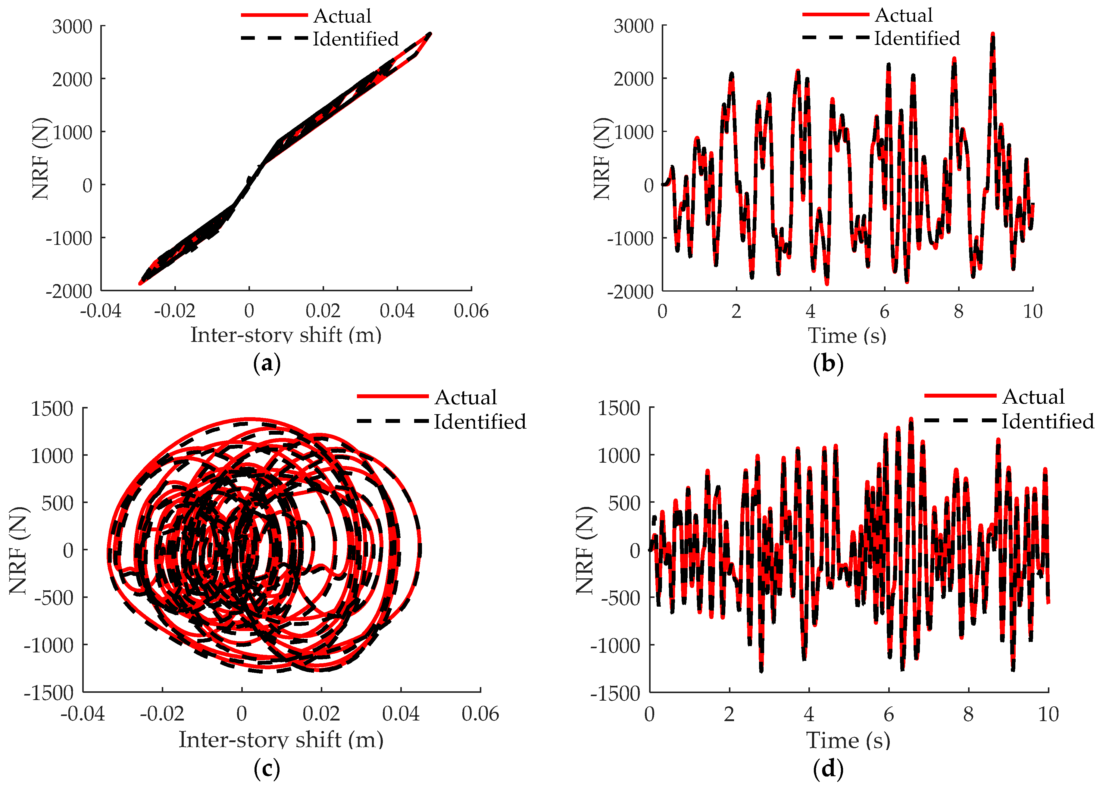
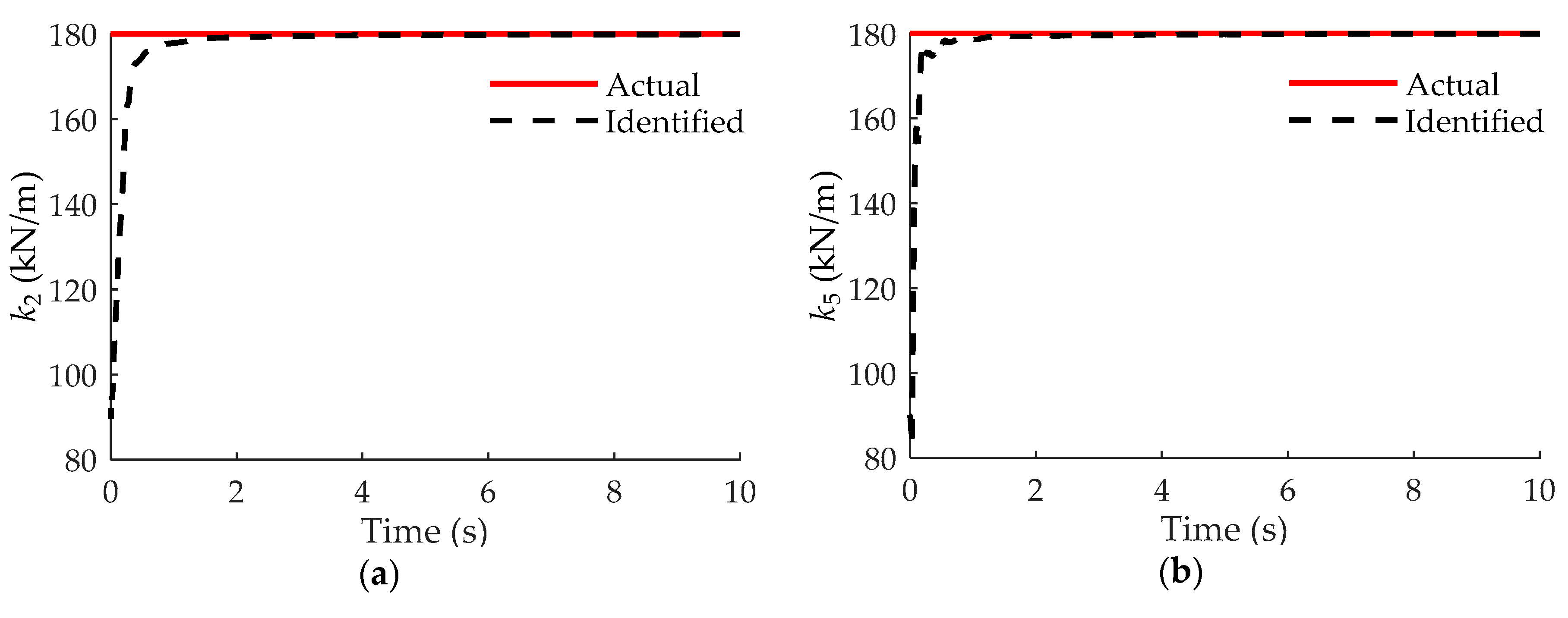
Based on the proposed approach, the unknown parameters could be identified as shown in Table 3. Clearly, the relative errors were quite small. Figure 7 gives the identified k1 and k4 as examples. It can be seen that the identified results can converge to the actual ones fast. Moreover, the NRFs provided by SMA damper and MR damper are identified and plotted in Figure 8 as dashed lines, whereas the theoretical ones are shown as solid lines. It can be observed the identified NRFs are all close to the actual ones.
4. Conclusions
In this paper, a model-free NRF identification approach was proposed basing on the principle of EKF. The NRFs provided by the nonlinear components such as the MR damper and SMA damper were treated as ‘unknown fictitious input’, and thus, no prior assumptions or approximations for the NRF model were required. A modified version of observation equation was obtained on the basis of the usage of a projection matrix. The recursive solution of the proposed approach was analytically derived. The structural parameters, including the stiffness and damping coefficients, were identified at each time step. The NRFs were also identified by means of LSE at the same time. The effectiveness and robustness of the proposed approach was numerically validated via a six-story building structure equipped with MR damper and/or SMA damper. A further comparison of the proposed approach with the PSPM method was made to demonstrate the reliability of the proposed approach for the identification of NRFs around the unsmooth points. The results show that the proposed approach is capable of satisfactorily identifying the structural parameters and unknown NRFs provided by the nonlinear components.
Although no prior knowledge of NRF model is required, the proposed approach should be performed under the condition that the influence matrix ηu associated with NRFs is available. Nonlinearities may often be located easily, at least for simple structures [3]. However, for complex structural systems, it is difficult to precisely determine the spatial localization of nonlinearities. Therefore, further research can be conducted towards the model-free NRF identification without the assumption of influence matrix being available.
Author Contributions
J.H. presented the framework of the proposed approach and wrote the paper; X.Z. and M.Q. gave the numerical examples for the validation of the proposed approach and participated in paper revision; B.X. showed the suggestions for the development of the algorithm and polished the manuscript.
Funding
The authors gratefully acknowledge the financial support from the National Natural Science Foundation of China through grant No. 751201239. The support from the Natural Science Foundation of Hunan Province (No. 2018JJ3054) and the Fundamental Development Funds for Young Researchers of Hunan University (No. 531107050912) are also greatly appreciated.
Conflicts of Interest
The authors declare no conflict of interest.
References
- Fan, W.; Qiao, P.Z. Vibration-based damage identification methods: A review and comparative study. Struct. Health Monit. 2011, 10, 83–111. [Google Scholar] [CrossRef]
- Xu, Y.L.; He, J. Smart Civil Structures; CRC Press: Boca Raton, FL, USA, 2017; pp. 333–389. [Google Scholar]
- Kerschen, G.; Worden, K.; Vakakis, A.F.; Golinval, J. Past, present and future of nonlinear system identification in structural dynamics. Mech. Syst. Signal Proc. 2006, 20, 505–592. [Google Scholar] [CrossRef]
- Kerschen, G.; Noël, J.P. Nonlinear system identification in structural dynamics: 10 more years of progress. Mech. Syst. Signal Proc. 2017, 83, 2–35. [Google Scholar]
- Worden, K.; Tomlinson, G.R. Nonlinearity in Structural Dynamics; IOP Publishing Ltd.: Bristol, UK, 2001; pp. 301–350. [Google Scholar]
- Di Massa, G.; Russo, R.; Strano, S.; Terzo, M. System structure identification and adaptive control of a seismic isolator test rig. Mech. Syst. Signal Proc. 2013, 40, 736–753. [Google Scholar] [CrossRef]
- Pagano, S.; Russo, R.; Strano, S.; Terzo, M. Non-linear modelling and optimal control of a hydraulically actuated seismic isolator test rig. Mech. Syst. Signal Proc. 2013, 35, 255–278. [Google Scholar] [CrossRef]
- Zaghari, B.; Rustighi, E.; Tehrani, M.G. Improved Modelling of a Nonlinear Parametrically Excited System with Electromagnetic Excitation. Vibration 2018, 1, 157–171. [Google Scholar] [CrossRef]
- Zhang, P.; Huo, L.; Song, G. Impact fatigue of viscoelastic materials subjected to pounding. Appl. Sci. 2018, 8, 117. [Google Scholar] [CrossRef]
- Kaloop, M.R.; Hu, J.W.; Bigdeli, Y. Identification of the response of a controlled building structure subjected to seismic load by using nonlinear system models. Appl. Sci. 2016, 6, 301. [Google Scholar] [CrossRef]
- Yang, J.N.; Lin, S.; Huang, H.W.; Zhou, L. An adaptive extended Kalman filter for structural damage identification. Struct. Control Health Monit. 2006, 13, 849–867. [Google Scholar] [CrossRef]
- Wu, M.; Smyth, A.W. Application of the unscented Kalman filter for real-time nonlinear structural system identification. Struct. Control Health Monit. 2007, 14, 971–990. [Google Scholar] [CrossRef]
- Lei, Y.; Wu, Y.; Li, T. Identification of nonlinear structural parameters under limited input and output measurements. Int. J. Nonlinear Mech. 2012, 47, 1141–1146. [Google Scholar] [CrossRef]
- Ding, Y.; Zhao, B.Y.; Wu, B. Structural system identification with extended Kalman filter and orthogonal decomposition of excitation. Math. Probl. Eng. 2014, 2014, 987694. [Google Scholar] [CrossRef]
- Ebrahimian, H.; Rodrigo Astroza, R.; Conte, J.P. Extended Kalman filter for material parameter estimation in nonlinear structural finite element models using direct differentiation method. Earth. Eng. Struct. Dyn. 2015, 44, 1495–1522. [Google Scholar] [CrossRef]
- Lei, Y.; Hua, W.; Luo, S.; He, M. Detection and parametric identification of structural nonlinear restoring forces from partial measurements of structural responses. Struct. Eng. Mech. 2015, 54, 291–304. [Google Scholar] [CrossRef]
- Liu, J.; Lei, Y.; He, M. A two-stage parametric identification of strong nonlinear structural systems with incomplete response measurements. Int. J. Struct. Stab. Dyn. 2016, 16, 1640022. [Google Scholar] [CrossRef]
- Jin, C.; Jang, S.; Sun, X. An integrated real-time structural damage detection method based on extended Kalman filter and dynamic statistical process control. Adv. Struct. Eng. 2017, 20, 549–563. [Google Scholar] [CrossRef]
- Xiao, M.; Zhang, Y.; Wang, Z. An adaptive three-stage extended Kalman filter for nonlinear discrete-time system in presence of unknown inputs. ISA Trans. 2018, 75, 101–117. [Google Scholar] [CrossRef]
- Astroza, R.; Alessandri, A.; Conte, J.P. A dual adaptive filtering approach for nonlinear finite element model updating accounting for modeling uncertainty. Mech. Syst. Signal Proc. 2019, 115, 782–800. [Google Scholar] [CrossRef]
- Astroza, R.; Ebrahimian, H.; Conte, J.P. Performance comparison of Kalman−based filters for nonlinear structural finite element model updating. J. Sound Vib. 2019, 438, 520–542. [Google Scholar] [CrossRef]
- Masri, S.F.; Caughey, T.K. A nonparametric identification technique for nonlinear dynamic problems. J. Appl. Mech. 1979, 46, 433–447. [Google Scholar] [CrossRef]
- Masri, S.F.; Sassi, H.; Caughey, T.K. A nonparametric identification of nearly arbitrary nonlinear systems. J. Appl. Mech. 1982, 49, 619–628. [Google Scholar] [CrossRef]
- Masri, S.F.; Miller, R.K.; Saud, A.F.; Caughey, T.K. Identification of nonlinear vibrating structures; part I: Formulation. J. Appl. Mech. 1987, 109, 918–922. [Google Scholar] [CrossRef]
- Masri, S.F.; Miller, R.K.; Saud, A.F.; Caughey, T.K. Identification of nonlinear vibrating structures; part II: Application. J. Appl. Mech. 1987, 109, 923–929. [Google Scholar] [CrossRef]
- Worden, K. Data processing and experiment design for the restoring force surface method, part I: Integration and differentiation of measured time data. Mech. Syst. Signal Proc. 1990, 4, 295–319. [Google Scholar] [CrossRef]
- Worden, K. Data processing and experiment design for the restoring force surface method, part II: Choice of excitation signal. Mech. Syst. Signal Proc. 1990, 4, 321–344. [Google Scholar] [CrossRef]
- Masri, S.F.; Tasbihgoo, F.; Caffrey, J.P.; Smyth, A.W.; Chassiakos, A.G. Data-based model-free representation of complex hysteretic MDOF systems. Struct. Control Health Monit. 2006, 13, 365–387. [Google Scholar] [CrossRef]
- Xu, B.; He, J.; Masri, S.F. Data-based Identification of nonlinear restoring force under spatially incomplete excitations with power series polynomial model. Nonlinear Dyn. 2012, 67, 2063–2080. [Google Scholar] [CrossRef]
- He, J.; Xu, B.; Masri, S.F. Restoring force and dynamic loadings identification for a nonlinear chain-like structure with partially unknown excitations. Nonlinear Dyn. 2012, 69, 231–245. [Google Scholar] [CrossRef]
- Xu, B.; He, J.; Dyke, S.J. Model-free nonlinear restoring force identification for SMA dampers with double Chebyshev polynomials: Approach and validation. Nonlinear Dyn. 2015, 82, 1507–1522. [Google Scholar] [CrossRef]
- Cesarano, C.; Fornaro, C. Operational identities on generalized two-variable Chebyshev polynomials. Int. J. Pure Appl. Math. 2015, 100, 59–74. [Google Scholar] [CrossRef]
- Cesarano, C.; Fornaro, C. A note on two-variable Chebyshev polynomials. Georgian Math J. 2017, 24, 339–349. [Google Scholar]
- Xu, B.; He, J.; Masri, S.F. Data-based model-free hysteretic restoring force and mass identification for dynamic systems. Comput. Aided Civ. Infrastruct. Eng. 2015, 30, 2–18. [Google Scholar] [CrossRef]
- Lei, Y.; Luo, S.J.; He, M.Y. Identification of model-free structural nonlinear restoring forces using partial measurements of structural responses. Adv. Struct. Eng. 2017, 20, 69–80. [Google Scholar] [CrossRef]
- Su, H.; Yang, X.; Liu, L.; Lei, Y. Identifying nonlinear characteristics of model-free MR dampers in structures with partial response data. Measurement 2018, 130, 362–371. [Google Scholar] [CrossRef]
- Yuan, T.C.; Yang, J.; Chen, L.Q. Nonparametric identification of nonlinear piezoelectric mechanical systems. J. Appl. Mech. 2018, 85, 111008. [Google Scholar] [CrossRef]
- Ondra, V.; Sever, I.A.; Schwingshackl, C.W. A method for non-parametric identification of non-linear vibration systems with asymmetric restoring forces from a resonant decay response. Mech. Syst. Signal Proc. 2019, 114, 239–258. [Google Scholar] [CrossRef]
- Worden, K.; Staszewski, W.J.; Hensman, J.J. Natural computing for mechanical systems research: A tutorial overview. Mech. Syst. Signal Proc. 2011, 25, 4–111. [Google Scholar] [CrossRef]
- Zhou, Q.; Qu, W.L. Two mechanic models for magnetorheological damper and corresponding test verification. Earthq. Eng. Eng. Vib. 2002, 22, 144–150. [Google Scholar]
Figure 1.
Building structure equipped with magnetorheological (MR) damper.

Figure 2.
The identified stiffness (building with MR damper): (a) first floor; (b) third floor.
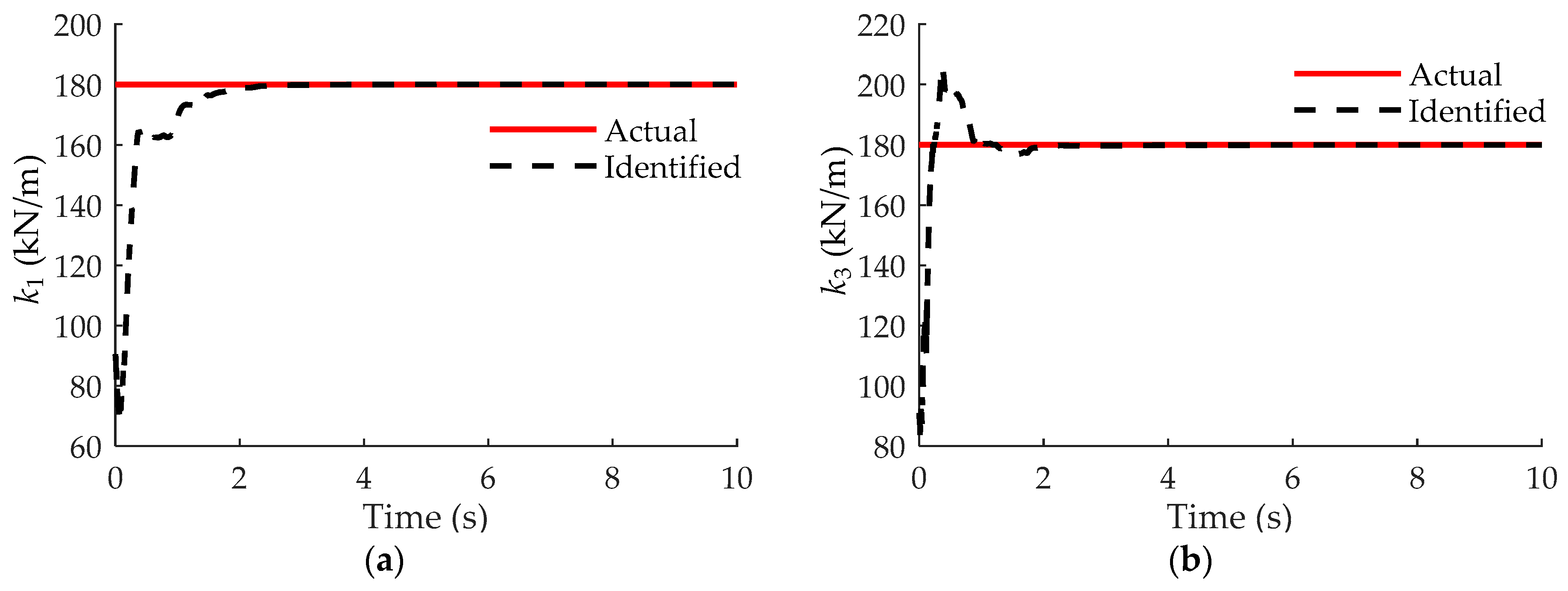
Figure 3.
Comparison of the identified MR damper force: (a) Hysteretic loop; (b) Time history of nonlinear restoring force (NRF).
Figure 3.
Comparison of the identified MR damper force: (a) Hysteretic loop; (b) Time history of nonlinear restoring force (NRF).
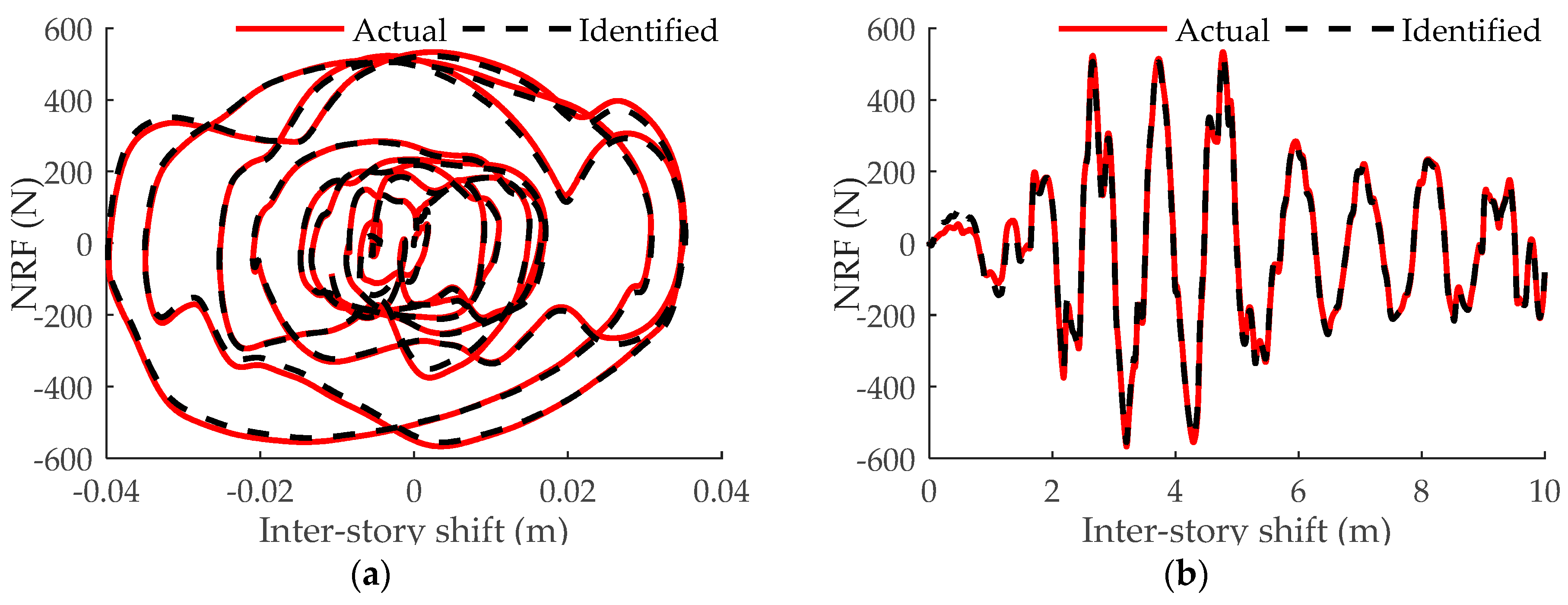
Figure 4.
NRF provided by shape memory alloy (SMA) damper.
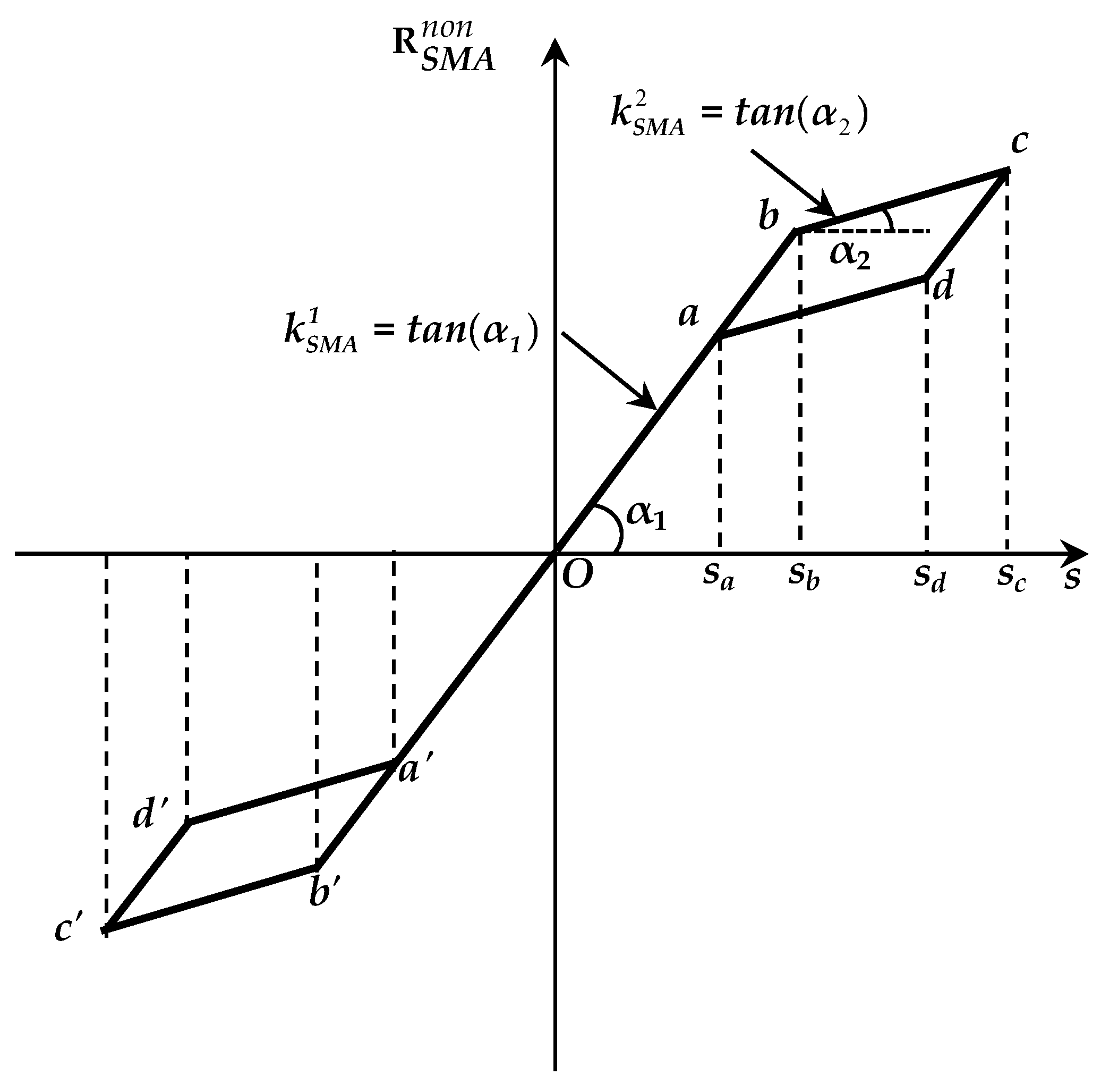
Figure 5.
The identified stiffness (building with SMA damper): (a) second floor; (b) fifth floor.

Figure 6.
Comparison of SMA damper force: (a) hysteretic loop; (b) time history of the identified error.
Figure 6.
Comparison of SMA damper force: (a) hysteretic loop; (b) time history of the identified error.

Figure 7.
The identified stiffness (building with SMA damper and MR damper): (a) first floor; (b) fourth floor.
Figure 7.
The identified stiffness (building with SMA damper and MR damper): (a) first floor; (b) fourth floor.
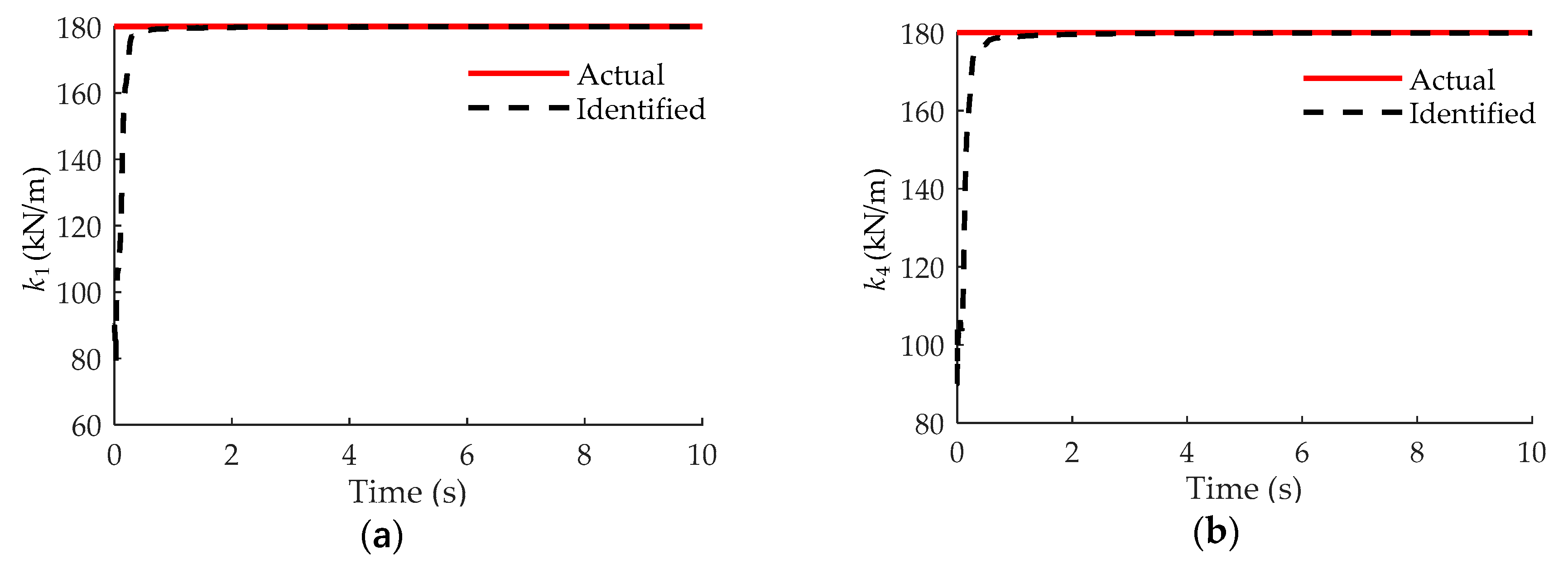
Figure 8.
Comparison of NRFs: (a) hysteretic loop of SMA damper; (b) time history of NRF by SMA damper; (c) hysteretic loop of MR damper; (d) time history of NRF by MR damper.
Figure 8.
Comparison of NRFs: (a) hysteretic loop of SMA damper; (b) time history of NRF by SMA damper; (c) hysteretic loop of MR damper; (d) time history of NRF by MR damper.

Table 1.
The identified results of building structure equipped with MR damper.
| Parameters | Actual | Identified | Error (%) | Parameters | Actual | Identified | Error (%) |
|---|---|---|---|---|---|---|---|
| k1 (kN/m) | 180.00 | 180.05 | 0.03 | k5 (kN/m) | 180.00 | 179.47 | −0.29 |
| k2 (kN/m) | 180.00 | 180.76 | 0.42 | k6 (kN/m) | 180.00 | 179.84 | −0.09 |
| k3 (kN/m) | 180.00 | 179.94 | -0.04 | α | 0.2644 | 0.2662 | 0.67 |
| k4 (kN/m) | 180.00 | 180.24 | 0.13 | β | 2.578 × 10⁻³ | 2.565 × 10⁻³ | −0.30 |
Table 2.
The identified results of building structure equipped with SMA damper.
| Parameters | Actual | Identified | Error (%) | Parameters | Actual | Identified | Error (%) |
|---|---|---|---|---|---|---|---|
| k1 (kN/m) | 180.00 | 179.92 | −0.05 | k5 (kN/m) | 180.00 | 179.94 | −0.04 |
| k2 (kN/m) | 180.00 | 179.88 | −0.06 | k6 (kN/m) | 180.00 | 179.83 | −0.10 |
| k3 (kN/m) | 180.00 | 179.84 | −0.09 | α | 0.2644 | 0.2643 | −0.04 |
| k4 (kN/m) | 180.00 | 179.90 | −0.06 | β | 2.578 × 10⁻³ | 2.591 × 10⁻³ | 0.55 |
Table 3.
The identified results of structural parameters equipped with SMA and MR damper.
| Parameters | Actual | Identified | Error (%) | Parameters | Actual | Identified | Error (%) |
|---|---|---|---|---|---|---|---|
| k1 (kN/m) | 180.00 | 179.96 | −0.02 | k5 (kN/m) | 180.00 | 179.98 | −0.01 |
| k2 (kN/m) | 180.00 | 179.94 | −0.03 | k6 (kN/m) | 180.00 | 179.86 | −0.08 |
| k3 (kN/m) | 180.00 | 179.95 | −0.03 | α | 0.2644 | 0.2642 | −0.07 |
| k4 (kN/m) | 180.00 | 179.92 | −0.05 | β | 2.578 × 10⁻³ | 2.589 × 10⁻³ | 0.31 |
© 2019 by the authors. Licensee MDPI, Basel, Switzerland. This article is an open access article distributed under the terms and conditions of the Creative Commons Attribution (CC BY) license (http://creativecommons.org/licenses/by/4.0/).
Share and Cite
MDPI and ACS Style
He, J.; Zhang, X.; Qi, M.; Xu, B. Model-Free Identification of Nonlinear Restoring Force with Modified Observation Equation. Appl. Sci. 2019, 9, 306. https://doi.org/10.3390/app9020306
AMA Style
He J, Zhang X, Qi M, Xu B. Model-Free Identification of Nonlinear Restoring Force with Modified Observation Equation. Applied Sciences. 2019; 9(2):306. https://doi.org/10.3390/app9020306
Chicago/Turabian StyleHe, Jia, Xiaoxiong Zhang, Mengchen Qi, and Bin Xu. 2019. "Model-Free Identification of Nonlinear Restoring Force with Modified Observation Equation" Applied Sciences 9, no. 2: 306. https://doi.org/10.3390/app9020306
Note that from the first issue of 2016, this journal uses article numbers instead of page numbers. See further details here.