Deep Learning-Based Damage, Load and Support Identification for a Composite Pipeline by Extracting Modal Macro Strains from Dynamic Excitations

Featured Application

The proposed novel approach presented in this paper offers a highly effective and reliable scheme for damage detection and safety assessment of pipeline systems and can be incorporated as a practical and highly reliable structural health monitoring approach for the safe operationty of existing and new pipeline systems.

Abstract

Modal macro strain-based damage identification is a promising approach since it has the advantages of high sensitivity and effectiveness over other related methods. In this paper, a basalt fiber-reinforced polymer (BFRP) pipeline system is used for analysis by using long-gauge distributed fiber Bragg grating (FBG) sensors. Dynamic macro strain responses are extracted to form modal macro strain (MMS) vectors. Both longitudinal distribution and circumferential distribution plots of MMS are compared and analyzed. Results show these plots can reflect damage information of the pipeline based on the previous work carried out by the authors. However, these plots may not be good choices for accurate detection of damage information since the model is 3D and has different flexural and torsional effects. Therefore, by extracting MMS information in the circumferential distribution plots, a novel deep neural network is employed to train and test these images, which reflect the important and key information of modal variance in the pipe system. Results show that the proposed Deep Learning based approach is a promising way to inherently identify damage types, location of the excitation load and support locations, especially when the structural types are complicated and the ambient environment is changing.

1. Introduction

Building resilient, ecological and sustainable infrastructure systems is increasingly becoming important since these systems degrade with time and are prone to damage when they are subjected to natural hazards and other unexpected disturbances. Pipelines, such as gas and utility pipeline systems and networks, are some of the most critical components of civil infrastructure. Therefore, to meet the goal that they have highly reliable serviceability performance under general or unforeseen loading scenarios, they must be properly designed to resist damage and deterioration over their entire lifespans. More importantly, implementation and utilization of an effective structural health monitoring system to assure the safety and potential damage detection of pipeline systems is important. Structural health monitoring can be divided into three major components including damage identification and its associated feature characterization, algorithm interpretation for diagnosis and prognostics, and structural reliability and risk assessment [1,2,3]. In engineering applications, composite structures have several distinct advantages such as high strength/weight ratio and corrosion resistance property, especially under the freeze and thaw cycle effects. Some disadvantages of composite structures are that they are prone to matrix cracks, fiber breakage, and delamination. These problems and faults are usually invisible and may lead to catastrophic structural failures [4,5]. Design methods, manufacturing process, and quality control are common factors that may cause internal and external damage. Several main failure modes of fiber reinforced polymer composites (FRP) include temperature-induced failure, corrosion-induced failure, bend failure, tensile failure, stress failure, impact failure, attachment joint failure, improper installation, etc. These failure types are complex and are not easy to identify, localize and quantify especially when structures are subjected to joint effects of multiple factors.

Different monitoring and analytical approaches have been proposed and employed for damage identification. By employing an improved conjugated beam method (ICBM), distributed structural deformation was monitored when the structure was subjected to combined actions of loads, support settlements and temperature variations [6]. This method has also been used to identify the settlement and lateral displacement of a statically indeterminate shield tunnel [7]. A theory regarding a long gauge strain influence line coefficient was introduced to detect damage and evaluate the bearing capacity of a bridge [8].

For long-gauge fiber applications, overall bonding and point fixation methods were investigated experimentally to develop non-slippage optical fibers, and critical effective sensing length was further studied [9]. A type of long distance fiber based sensing and monitoring system was employed to collect vibration signal responses of soil around the pipeline, and classify different kinds of activities using an artificial neural network [10]. A hydrostatic leak test for a water pipeline was studied using a distributed optical fiber vibration sensing system, which was based on phase-sensitive optical time-domain reflectometer (OTDR) technology [11] and fatigue damage identification for composite pipeline systems using electrical capacitance sensors [12].

A modal macro-strain vector was proposed and verified as an efficient damage identification algorithm to localize damage for flexural structures by directly extracting modal parameters from the dynamic responses of macro-strain [13,14]. By using macro-strain based distributed sensing and high-density point sensing, a comprehensive comparison of macro-strain modes and displacement modes was presented [15]. Local parameters such as bending stiffness and the global parameters, such as mass density and rotational stiffness of support, were well identified by introducing these parameters in the objective function and updating the finite element model [16]. Further field validation was conducted in a steel stringer bridge with area sensing [17].

For civil and industrial structures, it is difficult to monitor the structural health state in real time when the types of structures are complicated and the signals measured from the structures are corrupted due to environmental noise. Therefore, it is necessary to propose a non-model based approach to identify structural damage. Deep learning can address this problem in a satisfactory way due to its superior adaptive learning of datasets.

A large and deep convolutional neural network (CNN) was employed to make a classification of 1.2 million high-resolution images [18]. Derivation and implementation of convolutional neural networks were presented [19]. A vibration-based damage detection and localization in real-time was proposed by using 1D convolutional neural networks [20,21,22,23,24]. A sparse coding algorithm was applied to a large number of unlabeled examples to train a feature extractor, and features were then used to be fed to a neural network classifier to distinguish various damage statuses of bridges [25]. To overcome challenges such as lighting and shadow changes, a type of convolutional neural network with deep architecture was used for detection of concrete cracks without directly extracting defect features [26]. Responses of a healthy and loosened connection structure were analyzed via wavelet coefficient differences to indicate damage of a steel structure [27,28]. Wavelets were used to detect spikes in the wavelet details of responses of a framed structure subjected to strong earthquake excitation, indicating damage occurrence [29]. A combined wavelets, neural networks, and Hilbert transform, inspired by the deep learning paradigm, was presented to form a new signal-processing algorithm [30]. This was further studied to identify the fault condition of a roller bearing using three types of deep neural network models such as deep Boltzmann machines, deep belief networks and stacked auto-encoders [31]. Compared with a traditional support vector machine and back-propagation neural network, conditions of the planetary gearbox could be detected effectively with the best diagnosis accuracy using deep convolutional neural networks [32]. By applying wide linear models and deep neural networks, joint wide and deep learning was employed to combine the benefits of both generalization and memorization capability for recommender systems [33]. Concrete slabs with induced damage were investigated by applying big data analytics in online structural health monitoring [34]. A multi-scale structural health monitoring system was constructed to monitor the health states and assess the serviceability of large-scale bridges by employing the Hadoop Ecosystem (MS-SHM-Hadoop). A Bayesian network was studied to evaluate the reliability of specific components according to serviceability and inter-component correlations [35] and a hybrid response surface method [36].

Unlike buildings or bridges, for pipeline systems damage usually initiates from the internal surface especially when the internal temperature is higher than external temperature. Micro damage, matrix cracking [37], delamination [38,39], Webepage [40], and fiber failure are the three stages that result in ultimate failure of FRP composite structure, and damages may probably initiate and concentrate inside the pipes rather than outside the surface. Previous studies have shown that by acquiring images from structural damage areas (mostly outside surfaces of structures), it may be good to distinguish the different health states of structures. Images captured from the external surface of pipelines may not be an appropriate way to identify damage.

While modal macro strain (MMS) is an effective way to reflect damage condition, it has been only demonstrated in a 1D beam model [13,14,15,16], and a 3D pipeline model has not been validated. This paper extracts the section feature of modal macro strain of pipelines and applies deep learning algorithm to classify and identify different damage cases, and identify loading location and support locations. This approach is proved as a promising way to identify structural damages especially for completed structural types or rugged environment. The two main theories used in this paper include modal macro strain theory and convolutional neural network. Modal macro strain theory is mainly used for inherently extracting sensitive information of structures, which is later regarded as MMS distribution plots. These plots and images are fed into convolutional neural network for identifying damage severity, load location and support locations.

2. Modal Macro Strain (MMS)-Based Monitoring Strategy

Modal macro strain within the long gauge sensor can be measured from the peak value of the power spectral density (PSD) of macro strain signals from distributed dynamic response when the pipeline is subjected to ambient excitation. The normalized modal macro strain vector can be used to identify damage efficiently. Generally, the excitation of pipeline structure is unknown, therefore, the macro strain frequency response function (FRF) extracted from the ratio between output macro strain signals and input signals is unknown. The macro strain FRF denoted by $H_{mp}^{\overline{\epsilon }}\left(\omega \right)$ can be viewed as a ratio between the measurement from the mth sensor and the signal excitation pth degree of freedom (DOF), and can be acquired by:

$$H_{mp}^{\overline{\epsilon }}\left(\omega \right)=\frac{{\overline{\epsilon }}_{\omega }\left(\omega \right)}{P_P\left(\omega \right)},$$

(1)

where the superscript $\overline{\epsilon }$ is macro strain, and $P_P\left(\omega \right)$ is the signal excitation measured at the pth point. By studying the relationship between frequency response function and power spectral density, the power spectral density of macro strain in the dynamical response for mth long gauge sensor can be denoted as:

$$S_m^{\overline{\epsilon }}\left(\omega \right)={\left|H_{mp}^{\overline{\epsilon }}\left(\omega \right)\right|}^2{S}_P\left(\omega \right),$$

(2)

where power spectral density of the excitation at the pth point can be denoted as $S_P\left(\omega \right)$. The above equation can be represented as the following for a specific mode:

$$S_m^{\overline{\epsilon }}\left({\omega }_r\right)={\left|H_{mp}^{\overline{\epsilon }}\left({\omega }_r\right)\right|}^2{S}_P\left({\omega }_r\right),$$

(3)

$$\frac{\sqrt{S_m^{\overline{\epsilon }}\left({\omega }_r\right)}}{\sqrt{S_P\left({\omega }_r\right)}}=A_{pr}\left|{\delta }_{mr}\right|,$$

(4)

where, ${\delta }_{mr}$ is the macro strain measured within the mth gauge length, and the corresponding macro strain modal constant is expressed as:

$$A_{pr}=\frac{{\varphi }_{pr}}{2M_r{\xi }_r{\omega }_r^2},$$

(5)

where ${\varphi }_{pr}$, $M_r$, ${\xi }_r$ and ${\omega }_r$ respectively represent rth displacement mode shape at pth DOF, rth damping ratio, and rth natural frequency.

Through extracting the macro strain response from the PSD of dynamic signal for every long-gauge macro strain sensor, the modal macro strain is normalized in regard to that in the supposed mth reference sensor, and it can be acquired by:

$$\left[\begin{array}{c}\frac{{\delta }_{1r}}{{\delta }_{mr}}\\ \frac{{\delta }_{2r}}{{\delta }_{mr}}\\ ⋮\\ 1\\ ⋮\\ \frac{{\delta }_{nr}}{{\delta }_{mr}}\end{array}\right]=\left[\begin{array}{c}\frac{\sqrt{S_1^{\overline{\epsilon }}\left({\omega }_r\right)}}{\sqrt{S_m^{\overline{\epsilon }}\left({\omega }_r\right)}}\\ \frac{\sqrt{S_2^{\overline{\epsilon }}\left({\omega }_r\right)}}{\sqrt{S_m^{\overline{\epsilon }}\left({\omega }_r\right)}}\\ ⋮\\ 1\\ ⋮\\ \frac{\sqrt{S_n^{\overline{\epsilon }}\left({\omega }_r\right)}}{\sqrt{S_m^{\overline{\epsilon }}\left({\omega }_r\right)}}\end{array}\right],$$

(6)

The above equation means that the dynamic macro strain extracted from the power spectral density from all long-gauge sensors uniquely determines the structural modal macro strain. The peak values of power spectrum density of dynamic macro strain identify the natural frequencies and modal macro strain. The reference sensor is necessarily chosen for comparative study. For undamaged cases, the ratio of power spectral density at ${\omega }_i$ of dynamic macro strain from target sensor to that of the reference sensor remains invariant. The ratio varies obviously if damage develops and occurs within the area that the target sensors cover.

The time history of the macro strain from mth sensor within L_m gauge length is expressed as:

$${\overline{\epsilon }}_m\left(t\right)=\frac{h}{L_m}\left({\nu }_i\left(t\right)-{\nu }_j\left(t\right)\right).$$

(7)

where the distance from the sensor location to inertial axis is denoted as h, while ${\nu }_i\left(t\right)$ and ${\nu }_j\left(t\right)$ respectively denote rotational degree at first node of first element (ith DOF) within the gauge and that at second node of last element (jth DOF) within the gauge.

3. Convolutional Neural Networks (CNN)

A convolutional neural network generally consists of both alternating convolution operation and sub-sampling operation, and the last layer is denoted as a general multi-layer network. Interspersed with sub-sampling layers, convolutional layers are established to increase computation efficiency and further improve configural and spatial invariance.

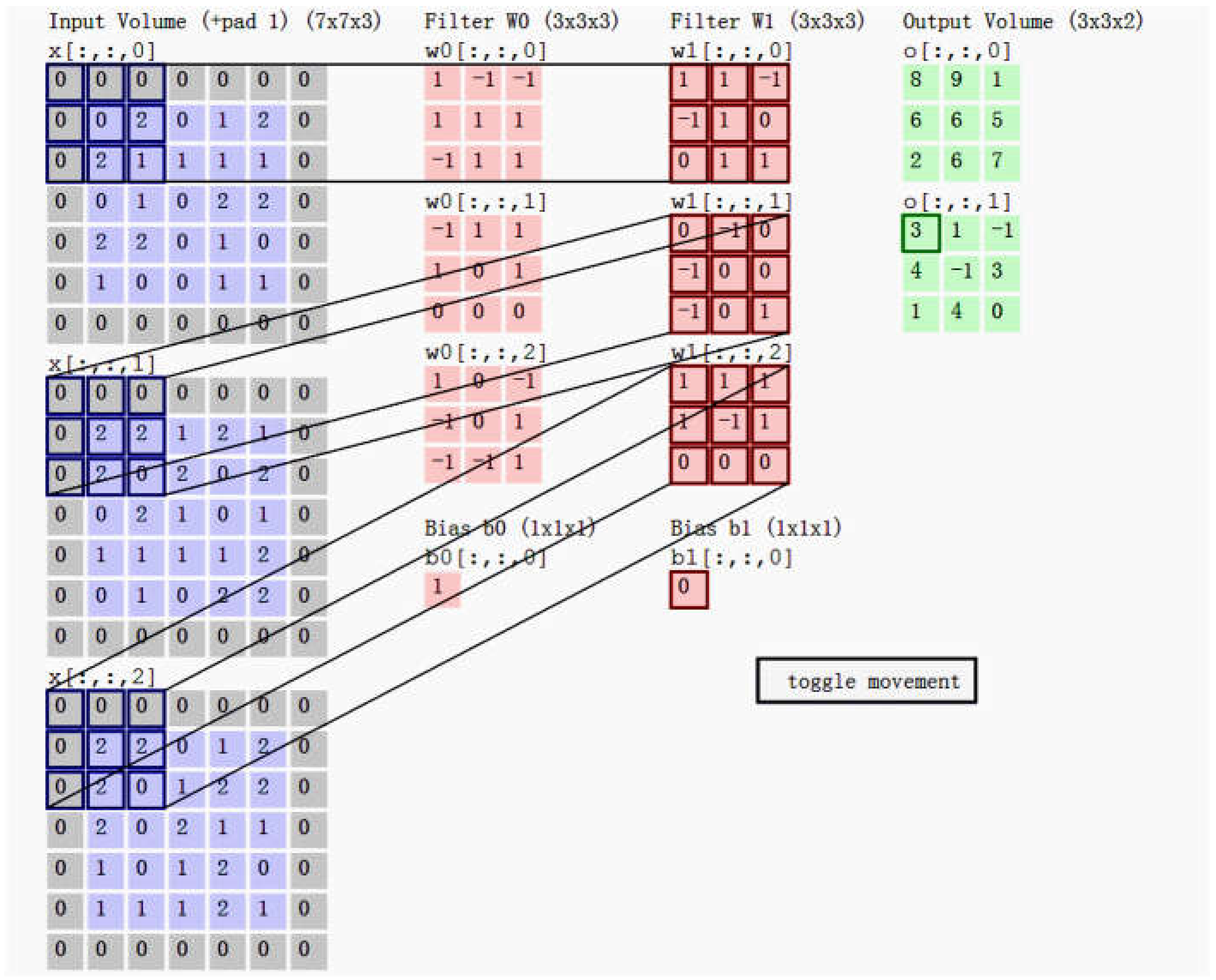
3.1. Convolution Layers

At a convolution layer, feature maps extracted from previous layers are convoluted with specific kernels and then activated to generate new feature maps. Multiple input feature maps are combined through the convolution operation until output is expressed as the following:

$${\mathbf{x}}_j^l=f\left({\displaystyle \sum }_{i\in M_j}{\mathbf{x}}_i^{l-1}*{\mathbf{k}}_{ij}^l+b_j^l\right).$$

(8)

where $M_j$ denotes a set of input feature maps, and each output feature map is added with an additive bias $b$. The input feature maps are convolved with distinct kernels for a particular output feature map.

3.2. Gradients in the Convolution Layers

The down-sampling layer $l+1$ follows the convolution layer $l$. For sensitivity computation, the nodes of units for the next layer $l+1$ are connected to the nodes of interest in the current layer $l$, and the connections between the two layers are associated with weights defined at layer $l+1$. We define that the “weights” at a down-sampling layer map are equivalent to $\beta$, and the previous result scaled by $\beta$ is computed to achieve ${\beta }^l$. Each map $j$ repeats the same computation in the convolutional layer with a paired map calculated in the subsampling layer:

$${\mathbf{\delta }}_j^l={\beta }_j^{l+1}\left(f^{\prime }\left({\mathbf{u}}_j^l\right)\circ up\left({\mathbf{\delta }}_j^{l+1}\right)\right),$$

(9)

where $up(\cdot )$ represents an operation of up-sampling which tiles each pixel in the input horizontally and vertically $n$ times in the output if the subsampling layer subsamples by a factor of $n$.

The gradients regarding bias $b_j$ and kernel weight ${\mathbf{k}}_{ij}^l$ are described as:

$$\frac{\partial E}{\partial b_j}={\displaystyle \sum }_{u,v}{\left({\mathbf{\delta }}_j^l\right)}_{uv},$$

(10)

$$\frac{\partial E}{\partial {\mathbf{k}}_{ij}^l}={\displaystyle \sum }_{u,v}{\left({\mathbf{\delta }}_j^l\right)}_{uv}{\left({\mathbf{p}}_i^{l-1}\right)}_{uv}$$

(11)

where ${\left({\mathbf{p}}_i^{l-1}\right)}_{uv}$ is the patch in ${\mathbf{x}}_i^{l-1}$ multiplied by ${\mathbf{k}}_{ij}^l$ via elementwise operation to calculate the element at $\left(u, v\right)$ in the output map ${\mathbf{x}}_j^l$ in the convolutional layer.

3.3. Sub-Sampling Layers

Down-sampled versions of the input maps are produced at a subsampling layer:

$${\mathbf{x}}_j^l=f\left({\beta }_j^{l}down\left(x_j^{l-1}\right)+b_j^l\right)$$

(12)

where $down(\cdot )$ denotes a sub-sampling operation.

3.4. Gradients in the Sub-Sampling Layers

Convolutional layers surround the subsampling layers above and below. Learnable parameters such as bias parameters $\beta$ and $b$ need to update:

$$\frac{\partial E}{\partial b_j}={\displaystyle \sum }_{u,v}{\left({\mathbf{\delta }}_j^l\right)}_{uv},$$

(13)

$$\frac{\partial E}{\partial {\beta }_j}={\displaystyle \sum }_{u,v}{\left({\mathbf{\delta }}_j^l\circ {\mathbf{d}}_j^l\right)}_{uv}.$$

(14)

3.5. Learning Combinations of Feature Maps

Let ${\alpha }_{ij}$ represents the weight that connects output map $j$ and input map $i$. The output map $j$ can be expressed as:

$$x_j^l=f\left({\displaystyle \sum }_{i=1}^{N_{in}}{\alpha }_{ij}\left(x_i^{l-1}*k_i^l\right)+b_j^l\right).$$

(15)

Subject to the constraints:

$${\displaystyle \sum }_i{\alpha }_{ij}=1 \mathrm{and} 0\le {\alpha }_{ij}\le 1.$$

(16)

The derivative of the soft max operation can be expressed as:

$$\frac{\partial {\alpha }_k}{\partial c_i}={\delta }_{ki}{\alpha }_i-{\alpha }_i{\alpha }_k.$$

(17)

While the derivative of error with respect to ${\alpha }_i$ and $c_i$ is given by:

$$\frac{\partial E}{\partial {\alpha }_i}=\frac{\partial E}{\partial u^l}\frac{\partial u^l}{\partial {\alpha }_i}={\displaystyle \sum }_{u, v}{\left({\mathbf{\delta }}^l\circ \left(x_i^{l-1}*k_i^l\right)\right)}_{uv}.$$

(18)

Herein, given inputs $\mathbf{u}$, ${\mathbf{\delta }}^l$ denote the sensitivity map with respect to an output map. A chain rule is employed to calculate the error gradients of the network regarding the underlying weights $c_i$:

$$\frac{\partial E}{\partial c_i}={\displaystyle \sum }_k\frac{\partial E}{\partial {\alpha }_k}\frac{\partial {\alpha }_k}{\partial c_i}={\alpha }_i\left(\frac{\partial E}{\partial {\alpha }_i}-{\displaystyle \sum }_k\frac{\partial E}{\partial {\alpha }_k}{\alpha }_k\right).$$

(19)

3.6. Enforcing Sparse Combinations

The distribution of weights ${\alpha }_i$ is imposed with sparseness constraints for a given map by incorporating a regularization penalty term $\mathsf{\Omega }\left(\alpha \right)$ into final error function. The regularization penalty $\mathsf{\Omega }\left(\alpha \right)$ can be derived as:

$$\frac{\partial \mathsf{\Omega }}{\partial {\alpha }_i}=\mathsf{\lambda }sign\left({\alpha }_i\right),$$

(20)

$$\frac{\partial \mathsf{\Omega }}{\partial c_i}={\displaystyle \sum }_k\frac{\partial \mathsf{\Omega }}{\partial {\alpha }_k}\frac{\partial {\alpha }_k}{\partial c_i}=\mathsf{\lambda }\left(\left|{\alpha }_i\right|-{\alpha }_i{\displaystyle \sum }_k\left|{\alpha }_k\right|\right).$$

(21)

Some examples are given to explain convolution and pooling processes, in the convolution operation, and we can see from Figure 1 that, the input data is composed of $a 7\times 7\times 3$ dataset, where $7\times 7$ represents width and height pixels, and 3 represents R, G, B color channels.

Filter W0 and filter W1 are two different filters. The stride is two, indicating that the window extracts $3\times 3$ local data, and strides two steps for each time. Zero padding = 1. With the left window moving smoothly, the filters convolve by using different local data covered by the window. Respectively, two filters are used to calculate convolution operation and two groups of results are shown.

In the convolutional neural network, filters (neurons with a group of fixed weights) are used to operate convolution for local input data. After calculating the data in each window, the data window moves smoothly with a specific stride, until the convolution operation is finished. There are a few parameters that need to be figured out:

(1)

Depth: the number of neurons (filters), determining the depth,

(2)

Stride: the number of stride covering through the data,

(3)

Zero padding: Supplement a few zeros to make the window more from the initial location to the end of the dataset.

Figure 2 is max pooling operation, which means taking the maximum value of the specific data window area. The other pooling method is average pooling in the CNN algorithm, i.e., take the average value of the specific data window area. Average pooling is applied in this paper.

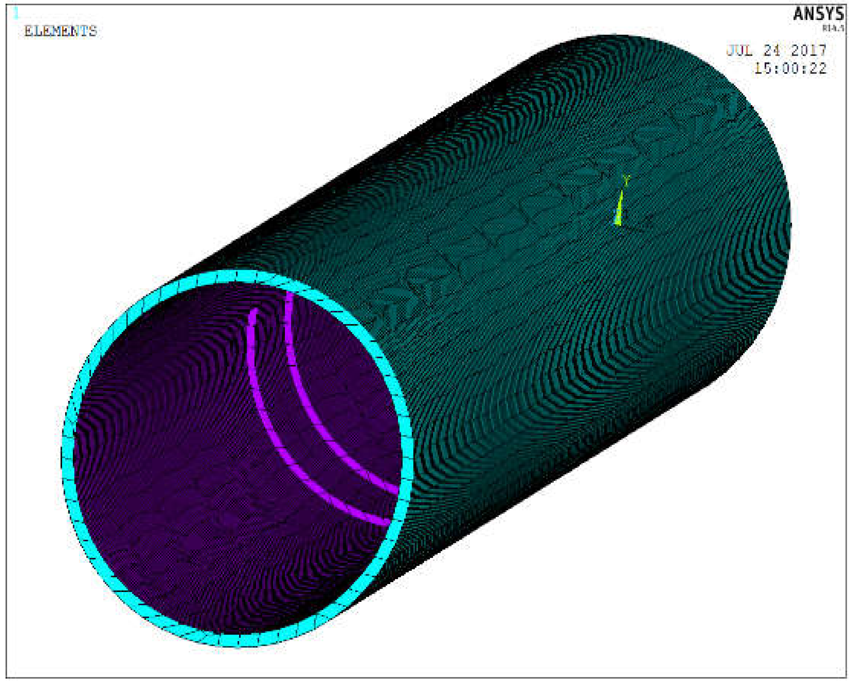
4. Pipeline System Modeling

A basalt fiber reinforced polymer (BFRP) composite pipeline finite element model is established as shown in Figure 3.

The ANSYS software version is R14.5 [41,42,43], and both tetrahedron meshing and free meshing are applied, the minimum element size is set 0.005 m. The element type of the composite pipeline is SHELL 181. The composite pipeline is 1 m long, the distribution of which is [−45, 45, −45, 45, −45]. The density of the model is 2.8 g/cm³. The internal radius is 0.04 m, and the external radius is 0.043 m. The boundaries are fixed for both two ends of the pipeline. Random excitation load is perpendicular to the wall of the pipe. Damage is modeled by reducing part of the stiffness of the pipeline. An enlarged view of damaged areas (marked in purple) in the pipeline is depicted in Figure 4.

Table 1. Basalt fiber reinforced polymer (BFRP) composite structural property.

Element Type	EX (Pa)	EY (Pa)	EZ (Pa)	PRXY	PRYZ	PRXZ	GXY (Pa)	GYZ (Pa)	GXZ (Pa)
SHELL181	93.5 × 109	20× 109	20× 109	0.28	0.3	0.28	8.5× 109	2.35× 109	2.35× 109

shows a detailed parameter list of structural property of BFRP composite pipeline.

Three damage levels are introduced, i.e., location: D1: 0.42–0.48 m, D2: 0.52–0.58 m, D3: 0.42–0.48 m + 0.52–0.58 m, all damages went across 180–360°, and are assumed to occur at the internal surface. The characteristics of the damages are:

• D1, D2: Same damage extent but different locations
• D3: Larger damage extent than D1 and D2 (D1 + D2)

Random excitation (Rand1) (−400~400 kN) is shown in Figure 5, and Figure 6 shows power spectral density (log) of random excitation. Sampling frequency is 1000 Hz, and the duration is 1 s. Twenty groups of random forces are loaded 0.2 m away from the right support of the pipeline, and for each loading, four different extents of damage are considered, and 10 modal macro strain feature maps are captured along the pipeline.

4.1. Modal Analysis of the Pipeline

Figure 7 shows 1st, 2nd and 3rd frequency of the intact pipeline.

Table 2. Structural frequency.

Frequency Order	D0 (Hz)	D1 (Hz)	D2 (Hz)	D3 (Hz)
1st order (Lateral Bending)	233.55	232.85	232.13	230.79
2nd order (Vertical Bending)	315.62	312.67	312.64	310.11
3rd order (Torsion)	824.38	822.90	822.48	820.85

lists all the values of frequency orders for different damage cases (D0–D3).

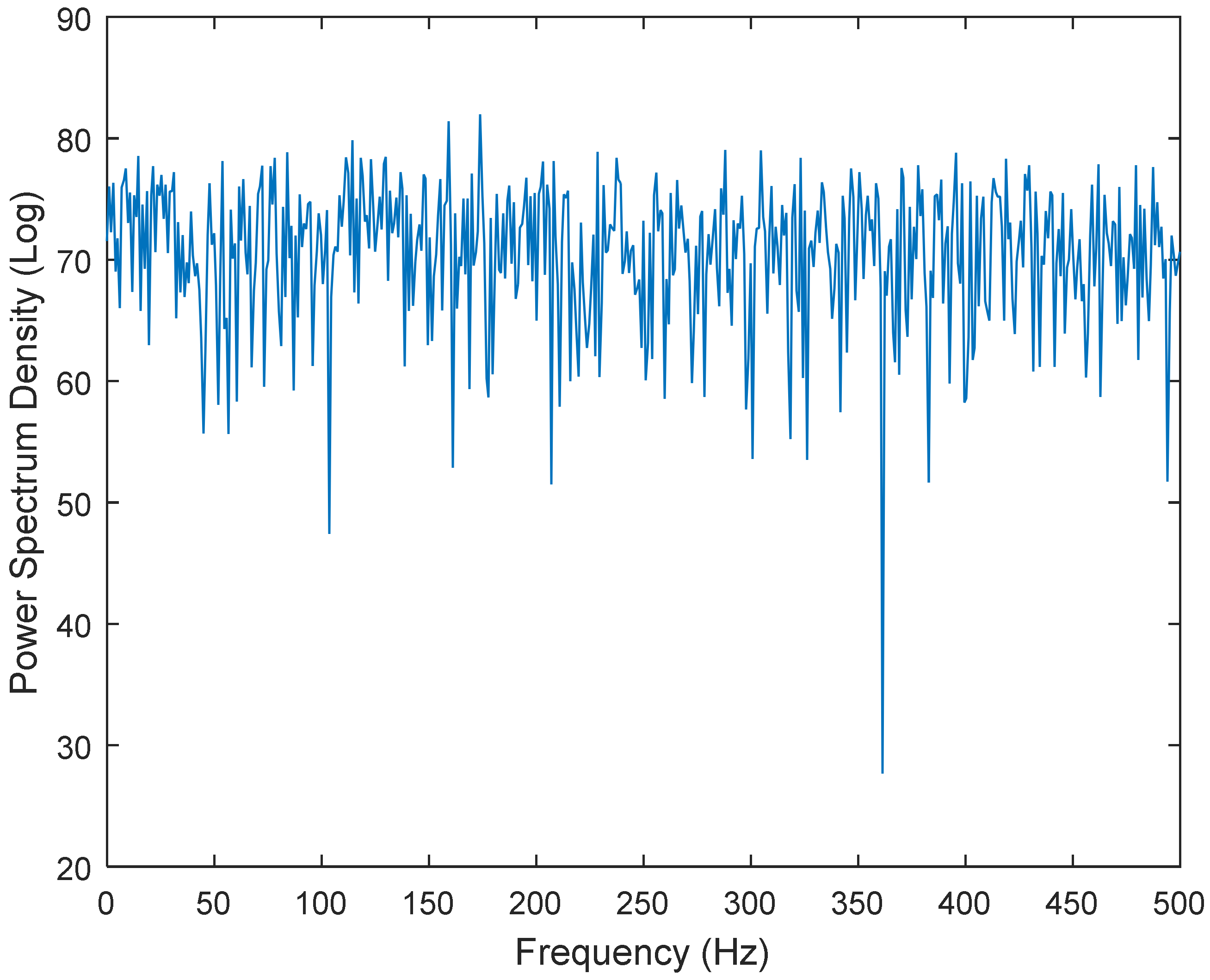
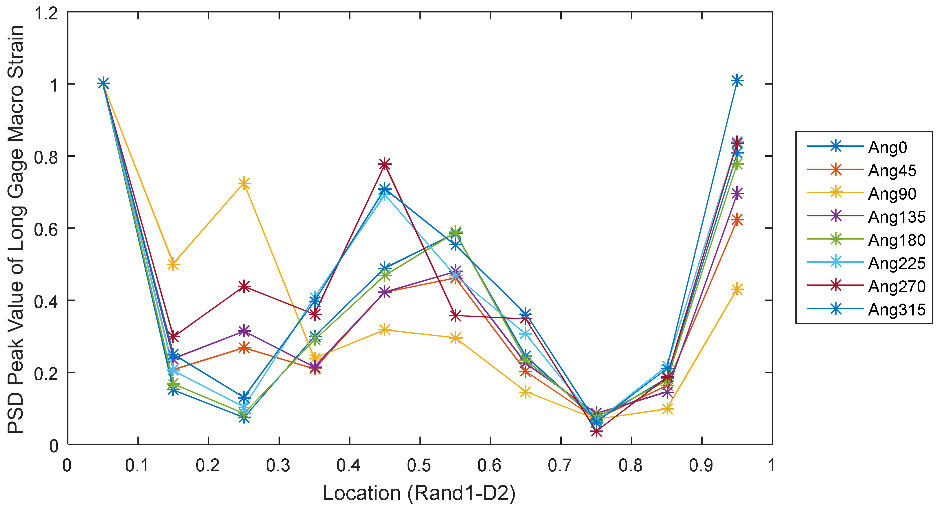
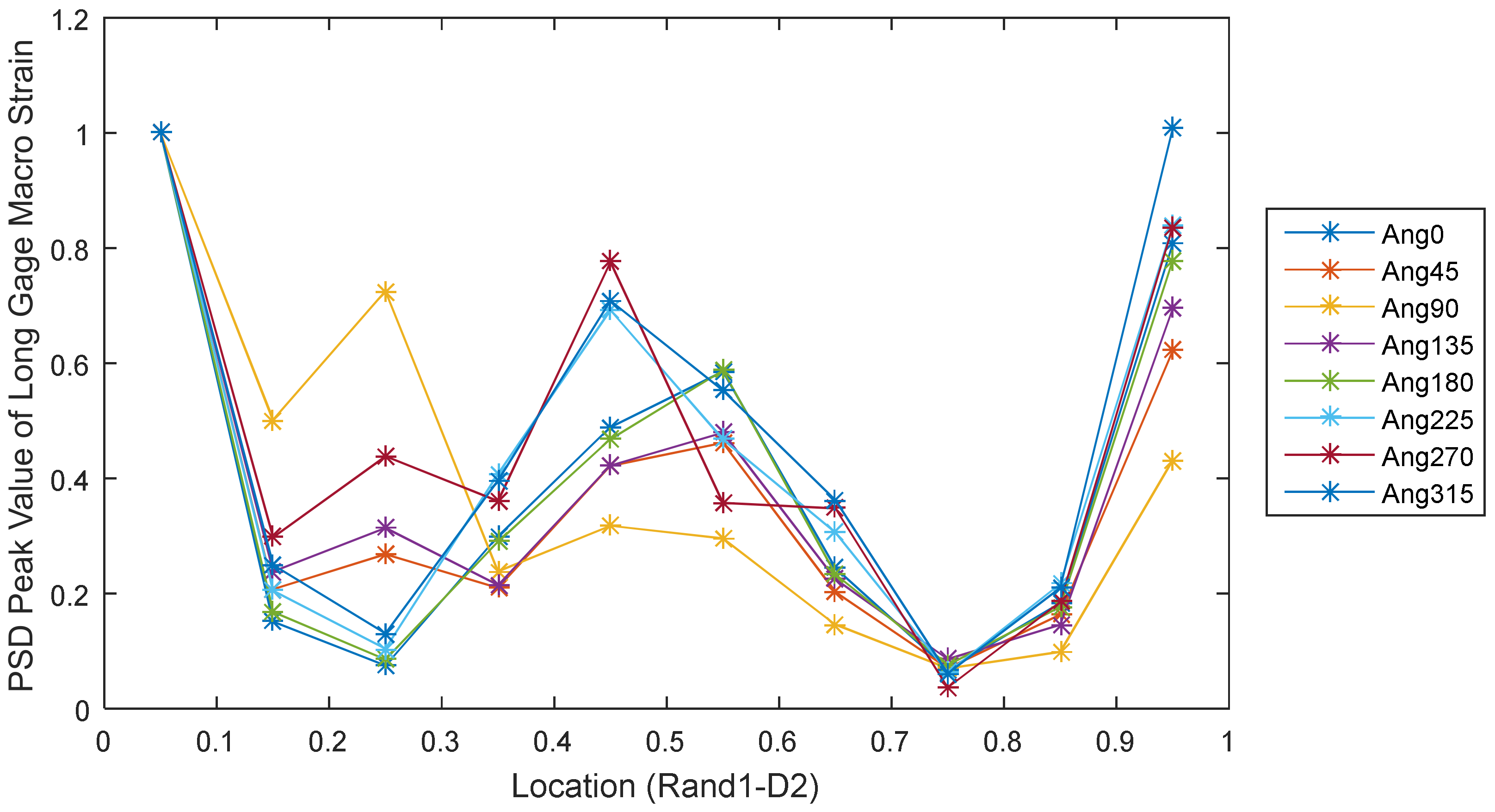
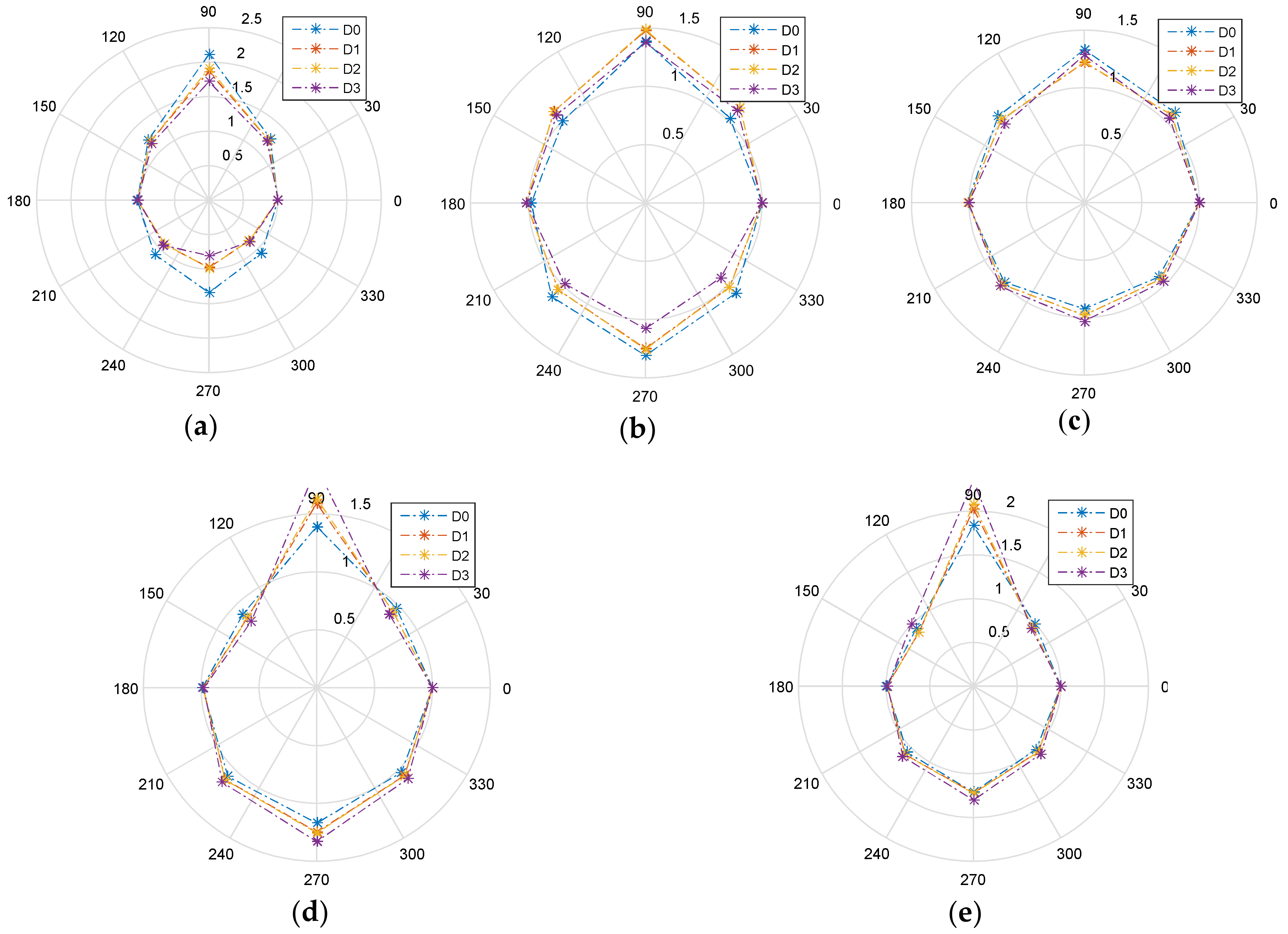
4.2. Identification Using Modal Macro Strain Method

Modal macro strain is calculated using the rotational displacements which are perpendicular to the radial direction measured by installed distributed angular displacement sensors, and then power spectral density is acquired via Fast Fourier Transform (FFT). By extracting the peak values, the modal macro strain relative values (normalized modal macro strain) are achieved. Grange length is chosen to be 0.1 m, and eight groups of macro strain dynamic responses are captured from eight angle direction (0°, 45°, 90°, 135°, 180°, 225°, 270°, 315°). Figure 8 shows the power spectral density of the dynamic strain response of the intact structure under the excitation of random force 1, and the power spectral density of macro strain dynamic responses is extracted from four groups of signals (angle 0°, 90°, 180°, 270°).

As shown in Figure 9, Figure 10, Figure 11 and Figure 12, modal macro strain vectors are extracted from eight-angles of each section, and 10 long gauges in the longitudinal direction of the pipeline are acquired. The reference macro strain location is Z = 0 m.

From Figure 9, we know that for the case of D0, two supports’ locations are well identified, and for angle = 90°, the MMS shows a hump compared with other cases, and the curves at 0.42–0.48 m and 0.52–0.58 m keep steady.

From Figure 10, we can see for the case of D1 (Location: 0.42–0.48 m), two supports’ locations are well identified, and for angle = 90°, the MMS shows a hump compared with other cases, and for angle = 0° and angle = 180° (the edges of damage areas), the MMS of the location 0.42–0.48 m shows a hump compared with other cases, but for the angle = 270° (the center of damage area), the MMS of the location 0.52–0.58 m shows a hump, this might be the result of an abrupt change of relative stiffness.

From Figure 11, we can see for the case of D2 (Location: 0.52–0.58 m), two supports’ locations are well identified, and for angle = 90°, the MMS shows a hump compared with other cases, and for angle = 0° and angle = 180° (the edges of damage areas), the MMS of the location 0.52–0.58 m shows a hump compared with other cases, but for the angle = 2700° (the center of damage area), the MMS of the location 0.42–0.48 m shows a hump, and this also might be as a result of abrupt change of relative stiffness.

From Figure 12, we can see for the case of D3 (Location: 0.42–0.48 m + 0.52–0.58 m), two supports’ locations are well identified, and for angle = 90°, the MMS shows a hump compared with other cases, and almost for all the angles, the MMSs of the location 0.42–0.48 m and 0.52–0.58 m are evident, especially for the case when angle = 2700°.

Figure 13 indicates the normalized modal macro strain distribution of 10 long gauges under rand1 excitation.

Figure 14 shows the normalized modal macro strain distribution of supports (Z = 0–0.1 m) of the pipeline under five random excitations.

From Figure 14, we can see that MMS distribution for different damage cases are not overlapped, and the shapes of MMS distribution tend to be circular. (Random excitation location is close to this support).

The case of MMS distribution (Z = 0–0.1 m) for different damage cases show that they are overlapped, and the shapes of MMS distribution tend to be circular. (Random excitation location is far away from this support).

Characteristics of MMS Plot of Cross Section at the Loading Point

Figure 15 and Figure 16 show the normalized modal macro strain distribution of external random excitations (Z = 0.1–0.2 m and Z = 0.2–0.3 m) of the pipeline under five random excitations.

From Figure 15 and Figure 16 we can see that the MMS distribution for different damage cases are almost overlapped, and the shapes of MMS distribution tend to be sharp. (Random excitation location is close to this gauge). The cases were also analyzed by studying the normalized modal macro strain distributions of external random excitations (Z = 0.4–0.5 m and Z = 0.5–0.6 m) of the pipeline under five random excitations. In these cases, MMS distributions for different damage cases are not overlapped, and the shapes of the MMS distributions tend to be circular. However, when the damage is more severe, the MMS distribution may not be larger. This is because the pipeline model is a 3D model and the damage can go through an area. Compared with 1D beam model and damage identification [13,14] this performs in a more complicated way.

4.3. Damage, Load and Support Identification Using CNN

In the previous section, MMS distributions were studied for the intact and damaged pipeline system. However, due to the 3D modeling and its inherent complexity, different damage levels can hardly be identified. Therefore, a more efficient way to extract the features of MMS distribution is employed for damage, load and support identification. The schematic diagram of the application of the convolutional neural network can be shown in Figure 17.

As discussed above, the convolution operation can be viewed as a neuron with fixed weights. The function of convolution layer is to identify local features of the previous layer, and the sampling layer is merging the similar features with the same feature.

▪

Cnnsetup: Each feature map is the number of feature map multiplied by the size of patch map for convolution. By moving a kernel window in the feature map, each neuron of feature map is traversed. The kernel window is composed of elements with the size of kernelsize × kernelsize. Each element is an independent weight, so there are kernelsize × kernelsize weights that need to be learned. Due to weight sharing, for the same feature map layer, the kernel window with the size of kernelsize × kernelsize has the same weights, which means weights are only determined by the kernel window. For different feature maps, the kernel windows are different, which means the weights are different.

▪

cnntrain: First reorder the sample, and randomly train and calculate the weights of network input and output. Then calculate the derivative of the error with respect to weights by the back propagation (BP) algorithm. Weight updating method will be used to update the network.

▪

Cnnff: Use the neural network to predict the input vector. First reorder the samples and then randomly train them. Samples are input to the network and are mapped for prediction. For each feature map of the last layer, the size of the feature map after convolution is: (feature map width-conv kernel width + 1) × (feature map height-conv kernel height + 1).

▪

cnnbp: The convolution layer is used for up-sampling and subsampling layer is used for down-sampling. The weights (size is onum × fvnum) between the last layer and the output neurons; where onum is the number of labels, and fvnum is the number of output neurons at the last layer.

▪

Cnnapplygrads: The Cnnapplygrads is used for weight updating. The training dataset is 256 × 256 × 6000, testing dataset is 256 × 256 × 800, labeled training dataset is 7 × 6000, and the labeled testing dataset is 7 × 800. The construction of the conventional neural network is 6c–2s–12c–2s (c: convolution layer, s: sub sampling layer), learning efficiency Alpha = 1, Batchsize = 50, and Numepoch = 1.

The superior characteristics of deep learning is that the outputs of intermediate layers can be used as another expression of data, therefore regarding it as the learned features through network adaptive learning, and these features can later be used for similarity comparison. The amounts of data can be used to effectively train parameters of deep learning network. In this study, the convolutional neural network includes two convolutional layers, two sub-sampling layers, and a full connection layer. Each layer tuned parameters and the corresponding weights. The input image size is 256 × 256.

The basic architecture of the connection of the convolutional layer and sub-sampling layer is depicted in Figure 18. C1 is a convolutional layer composed of six feature maps. By doing convolutional operation, the feature of the original signal can be enhanced and also reduce noise effects. Each neuron of the feature map is connected with 16 × 16 neighborhood of input images. The feature map size is 196 × 196. C1 has 156 tuned parameters (each filter has 16 × 16 unit parameters and a bias parameter, 6 filters in total, so (16 × 16 + 1) × 6 = 1542 parameters in total). One kernel is used between input and C1, so 1542 × (196 × 196) = 59,237,472 connections in total.

S2 is a sub-sampling layer. According to the local correlation principle of image, sub-sampling can be applied to images, thus decreasing data processing ability and retaining useful information. Two 98 × 98 feature maps are used. Each unit of feature map is connected with 8 × 8 neighborhood of C1. Sixteen inputs of each unit of S2 are added, multiplied by a tuned parameter with a tuned bias. The result can be calculated by sigmoid function. Tuned parameters and bias control the non-linearity of the sigmoid function. If these parameters are relatively small, the operation is as similar as linear operation. Sub-sampling is equivalent to fuzzy images by decreasing the pixels of the images. If these parameters are relatively larger, sub-sampling can be regarded as “or” or “and” operations with noise. 8 × 8 receptive field is not overlapped for each unit, therefore the size of each feature map in S2 is 1/4 of that of C1. S2 has (1 + 1) × 2 = 4 tuned parameters and (8 × 8 + 1) × 2 × (98 × 98) = 1,248,520 connections.

C3 and S4 have similar architectures, and output layers are composed of Euclidean radial basis function units. Images are fed into the network and the output $O_p=F_n\left(\cdots \left(F_2\left(F_1\left(X_p{W}^{\left(1\right)}\right)W^{\left(2\right)}\right)\right)\cdots W^{\left(n\right)}\right)$, and the error between practical output $O_p$ and desired output $Y_p$ can be calculated by back propagation with tuned weight parameters.

Table 3. Labeled dataset.

Label	1	2	3	4	5	6	7
Case	Support 1	Support 2	Excitation	D0	D1	D2	D3
Location	0–0.1 m	0.9–1 m	0.1–0.2 m/0.2–0.3 m	Other Cases	0.4–0.5 m	0.5–0.6 m	0.4–0.5 m/0.5–0.6 m

labels all the cases regarding two supports, excitation loads and different damage cases (D0–D3).

Table 4. Label settings for different damage cases.

Case	Str1	Str2	Str3	Str4	Str5	Str6	Str7	Str8	Str9	Str10
D0	label1	label3	label3	label4	label4	label4	label4	label4	label4	label2
D1	label1	label3	label3	label4	label5	label4	label4	label4	label4	label2
D2	label1	label3	label3	label4	label4	label6	label4	label4	label4	label2
D3	label1	label3	label3	label4	label7	label7	label4	label4	label4	label2

displays all the label settings for 10 strain gauge strain in the longitudinal direction for different damage cases.

Table 5. Identification testing results.

Label	1	2	3	4	5	6	7
Number	80	80	160	400	20	20	40
TPR	75 (93.75%)	77 (96.25%)	156 (97.5%)	388 (97%)	18 (90%)	18 (90%)	37 (92.5%)
TNR	704 (97.78%)	701 (97.36)	623 (97.34%)	379 (94.75%)	766 (98.21%)	764 (97.95%)	748 (98.42%)
FPR	16 (2.22%)	19 (2.64%)	17 (2.66%)	21 (5.25%)	14 (1.79%)	16 (2.05%)	12 (1.58%)
FNR	5 (6.25%)	3 (3.75%)	4 (2.5%)	12 (3%)	2 (10%)	2 (10%)	3 (7.5%)

Remark: true positive (TP): prediction is positive and the sample is positive. True negative (TN): prediction is negative and the sample is negative. False positive (FP): prediction is positive and the sample is negative. False negative (FN): prediction is negative and the sample is positive.

shows the damage, load and support identification results for seven labels with respect to true positive rate (TPR), true negative rate (TNR), false positive rate (FPR) and false negative rate (FNR).

Images are scaled to the same size 900 × 1200 × 3 and then 256 × 256 × 1 without any annotation.

For labeled dataset, the location for the specific case (Support 1, Support 2, Excitation, D0, D1, D2, D3) is labeled 1 while other locations are labeled 0.

Different evaluation rates can be calculated by:

(1)

True positive rate (TPR) = TP/(TP + FN),

(2)

True negative rate (TNR) = TN/(TN + FP),

(3)

False positive rate (FPR) = FP/(FP + TN),

(4)

False negative rate (FNR) = FN/(TP + FN).

Eight hundred testing datasets are employed to verify the effectiveness of convolutional neural network, and it is promising to apply CNN to the identification of different extents of damage, load excitation location and support location.

For engineering applications, to the best of the authors’ knowledge, most work presented in the literature use artificial neural network-related methods to process images taken from bridges, tunnels, pipes. The disadvantages of this method include the fact that images may not inherently reflect the structural health status, and even if these images are fed into convolutional neural network, the trained images may not have a good generalization ability to evaluate the test samples. By combining the modal macro strain method and convolutional neural network, the sensitive strain distribution information can be extracted and then fed it into convolutional neural network for training and testing. The combination of these two methods can be used effectively to solve actual practical problems in complex civil engineering structures based on the numerical and analytical results shown in this study. A composite pipeline prototype model also is being experimentally conducted at the National and Local Joint Research Center for Basalt Fiber Production and Application Technology to verify the effectiveness and applicability of the combined modal macro strain and convolutional neural network methods.

5. Conclusions

This paper first presented the basic theory of modal macro strain-based long gauge distributed sensing technology, and deep learning theory. Both longitudinal distribution and circumferential distribution of modal macro strain were investigated and results indicated some characteristics of damage extent, load excitation location and support location. Image-based damage identification using deep learning tools could only identify the external damage of structures while internal damage images could hardly be reflected if images were acquired from outside of the structures. As concluded, the other disadvantages of image-based damage identification is that these images may include the disturbances of noise, and different extents of light and shadows. The advantages of the work presented in this paper overcomes 1D beam-based damage identification; a 3D model was built to reflect the real status of structures. Combined with long gauge distributed sensing technology, modal macro strains were extracted from peak values of power spectral density from the dynamic responses of different locations of long gauges, and a convolutional neural network was applied to circumferential distribution plots of modal macro strain. Compared with direct methods of image extraction for damage identification, the proposed methodologies first study the plot distribution map of structural modal macro strains, which is a sensitive parameter to structural damage. Then by training and testing these “feature maps” using convolutional neural network, the extents of damages, external excitation location and support locations can be inherently identified. This is especially suitable for complicated structural types, complex and changing environments.

References

1. Lynch, J.P.; Farrar, C.R.; Michaels, J.E. Structural health monitoring: Technological advances to practical implementations. Proc. IEEE 2016, 104, 1508–1512. [Google Scholar] [CrossRef]
2. Ying, Z.; Mohammad, N.; Seyed, B.B.; Altabey, W.A. Mode shape based damage identification for a reinforced concrete beam using wavelet coefficient differences and multi-resolution analysis. J. Struct. Control Health Monit. 2017, 25, 1–41. [Google Scholar] [CrossRef]
3. Ying, Z.; Mohammad, N.; Altabey, W.A. Damage detection for a beam under transient excitation via three different algorithms. J. Struct. Eng. Mech. 2017, 63, 803–817. [Google Scholar] [CrossRef]
4. Kesavan, A.; John, S.; Herszberg, I. Strain-based structural health monitoring of complex composite structures. J. Struct. Health Monit. 2008, 7, 203–213. [Google Scholar] [CrossRef]
5. Altabey, W.A. An exact solution for mechanical behavior of BFRP Nano-thin films embedded in NEMS. J. Adv. Nano Res. 2017, 5, 337–357. [Google Scholar] [CrossRef]
6. Shen, S.; Wu, Z.; Yang, C.; Wan, C.; Tang, Y.; Wu, G. An improved conjugated beam method for deformation monitoring with a distributed sensitive fiber optic sensor. J. Struct. Health Monit. 2010, 9, 361–378. [Google Scholar] [CrossRef]
7. Shen, S.; Wu, Z.; Lin, M. Distributed settlement and lateral displacement monitoring for shield tunnel based on an improved conjugated beam method. J. Adv. Struct. Eng. 2013, 16, 1411–1425. [Google Scholar] [CrossRef]
8. Wu, B.; Wu, G.; Yang, C.; He, Y. Damage identification and bearing capacity evaluation of bridges based on distributed long-gauge strain envelope line under moving vehicle loads. J. Intell. Mater. Syst. Struct. 2016, 27, 2344–2358. [Google Scholar] [CrossRef]
9. Wu, Z.; Zhang, H.; Yang, C. Development and performance evaluation of non-slippage optical fiber as Brillouin scattering-based distributed sensors. J. Struct. Health Monit. 2010, 9, 413–431. [Google Scholar] [CrossRef]
10. Wang, L.; Wang, Y.H.; Xiao, X.L.; Yan, H.; Shi, G.S.; Wang, Q.R. A fiber-sensor-based long-distance safety monitoring system for buried oil pipeline. In Proceedings of the IEEE International Conference on Networking, Sensing and Control, Sanya, China, 6–8 April 2008; Volume 6, pp. 451–456. [Google Scholar] [CrossRef]
11. Wu, H.; Sun, Z.; Qian, Y.; Zhang, T.; Rao, Y. A hydrostatic leak test for water pipeline by using distributed optical fiber vibration sensing system. In Proceedings of the Fifth Asia-Pacific Optical Sensors Conference, International Society for Optics and Photonics, Jeju, Korea, 1 July 2015; Volume 1, p. 9655 (965543). [Google Scholar]
12. Ying, Z.; Mohammad, N.; Altabey, W.A.; Zhishen, W. Fatigue Damage Identification for Composite Pipeline Systems Using Electrical Capacitance Sensors. J. Smart Mater. Struct. 2018, 27, 085023. [Google Scholar] [CrossRef]
13. Tang, Y.; Wu, Z.; Yang, C.; Wu, G.; Wan, C. A model-free damage identification method for flexural structures using dynamic measurements from distributed long-gauge macro-strain sensors. J. Intell. Mater. Syst. Struct. 2014, 25, 1614–1630. [Google Scholar] [CrossRef]
14. Hong, W.; Wu, Z.; Yang, C.; Wan, C.; Wu, G. Investigation on the damage identification of bridges using distributed long-gauge dynamic macrostrain response under ambient excitation. J. Intell. Mater. Syst. Struct. 2012, 23, 85–103. [Google Scholar] [CrossRef]
15. Hong, W.; Zhang, J.; Wu, G.; Wu, Z. Comprehensive comparison of macro-strain mode and displacement mode based on different sensing technologies. Mech. Syst. Signal Process. 2015, 50, 563–579. [Google Scholar] [CrossRef]
16. Hong, W.; Wu, Z.; Yang, C.; Wu, G.; Zhang, Y. Finite element model updating of flexural structures based on modal parameters extracted from dynamic distributed macro-strain responses. J. Intell. Mater. Syst. Struct. 2015, 26, 201–218. [Google Scholar] [CrossRef]
17. Zhang, J.; Hong, W.; Tang, Y.; Yang, C.; Wu, G.; Wu, Z. Structural health monitoring of a steel stringer bridge with area sensing. J. Struct. Infrastruct. Eng. 2014, 10, 1049–1058. [Google Scholar] [CrossRef]
18. Krizhevsky, A.; Sutskever, I.; Hinton, G.E. Imagenet classification with deep convolutional neural networks. J. Adv. Neural Inf. Process. Syst. 2012, 1097–1105. [Google Scholar] [CrossRef]
19. Bouvrie, J. Notes on Convolutional Neural Networks; Center for Biological Learning, Department of Brain and Cognitive Sciences, Massachusetts Institute of Technology: Cambridge, MA, USA, 2006. [Google Scholar]
20. Altabey, W.A. Free vibration of basalt fiber reinforced polymer (FRP) laminated variable thickness plates with intermediate elastic support using finite strip transition matrix (FSTM) method. J. Vibroeng. 2017, 19, 2873–2885. [Google Scholar] [CrossRef]
21. Altabey, W.A. Prediction of natural frequency of basalt fiber reinforced polymer (FRP) laminated variable thickness plates with intermediate elastic support using artificial neural networks (ANNs) method. J. Vibroeng. 2017, 19, 3668–3678. [Google Scholar] [CrossRef]
22. Altabey, W.A. High performance estimations of natural frequency of basalt FRP laminated plates with intermediate elastic support using response surfaces method. J. Vibroeng. 2018, 20, 1099–1107. [Google Scholar] [CrossRef] [Green Version]
23. Al-Tabey, W.A. Vibration analysis of laminated composite variable thickness plate using finite strip transition matrix technique. In MATLAB Verifications MATLAB-Particular for Engineer; Kelly, B., Ed.; InTech: West Palm Beach, FL, USA, 2014; Volume 21, pp. 583–620. ISBN 980–953-307-1128-8. [Google Scholar]
24. Abdeljaber, O.; Avci, O.; Kiranyaz, S.; Gabbouj, M.; Inman, D.J. Real-time vibration-based structural damage detection using one-dimensional convolutional neural networks. J. Sound Vib. 2017, 388, 154–170. [Google Scholar] [CrossRef]
25. Guo, J.; Xie, X.; Bie, R.; Sun, L. Structural health monitoring by using a sparse coding-based deep learning algorithm with wireless sensor networks. J. Pers. Ubiquitous Comput. 2014, 18, 1977–1987. [Google Scholar] [CrossRef]
26. Cha, Y.J.; Choi, W.; Büyüköztürk, O. Deep learning-based crack damage detection using convolutional neural networks. J. Comput.-Aided Civ. Infrastruct. Eng. 2017, 32, 361–378. [Google Scholar] [CrossRef]
27. Pnevmatikos, N.G.; Blachowski, B.; Hatzigeorgiou, G.D.; Swiercz, A. Wavelet analysis based damage localization in steel frames with bolted connections. J. Smart Struct. Syst. 2016, 18, 1189–1202. [Google Scholar] [CrossRef]
28. Mohammad, N.; Haifegn, W.; Altabey, W.A.; Ahmad, I.H.S. A Modified Wavelet Energy Rate Based Damage Identification Method for Steel Bridges. Int. J. Sci. Technol. Sci. Iran. 2018. [Google Scholar] [CrossRef]
29. Pnevmatikos, N.G.; Hatzigeorgiou, G.D. Damage detection of framed structures subjected to earthquake excitation using discrete wavelet analysis. J. Bull. Earthq. Eng. 2017, 15, 227–248. [Google Scholar] [CrossRef]
30. Kanarachos, S.; Christopoulos, S.R.; Chroneos, A.; Fitzpatrick, M.E. Detecting anomalies in time series data via a deep learning algorithm combining wavelets, neural networks and Hilbert transform. Expert Syst. Appl. 2017, 85, 292–304. [Google Scholar] [CrossRef]
31. Chen, Z.; Deng, S.; Chen, X.; Li, C.; Sanchez, R.V.; Qin, H. Deep neural networks-based rolling bearing fault diagnosis. J. Microelectron. Reliab. 2017, 75, 327–333. [Google Scholar] [CrossRef]
32. Jing, L.; Wang, T.; Zhao, M.; Wang, P. An adaptive multi-sensor data fusion method based on deep convolutional neural networks for fault diagnosis of planetary gearbox. J. Sens. 2017, 17, 414. [Google Scholar] [CrossRef]
33. Cheng, H.T.; Koc, L.; Harmsen, J.; Shaked, T.; Chandra, T.; Aradhye, H.; Anderson, G.; Corrado, G.; Chai, W.; Ispir, M.; et al. Wide & deep learning for recommender systems. In Proceedings of the 1st Workshop on Deep Learning for Recommender Systems, Boston, MA, USA, 15 September 2016; ACM: New York, NY, USA; pp. 7–10. [Google Scholar]
34. Cai, G. Big Data Analytics in Structural Health Monitoring. Doctoral Dissertation, Vanderbilt University, Nashville, TN, USA, 2017. [Google Scholar]
35. Liang, Y.; Wu, D.; Liu, G.; Li, Y.; Gao, C.; Ma, Z.J.; Wu, W. Big data-enabled multiscale serviceability analysis for aging bridges. J. Digit. Commun. Netw. 2016, 2, 97–107. [Google Scholar] [CrossRef]
36. Ying, Z.; Mohammad, N.; Altabey, W.A.; Naiwei, L. Reliability Evaluation of a Laminate Composite Plate Under Distributed Pressure Using a Hybrid Response Surface method. Int. J. Reliab. Qual. Saf. Eng. 2017, 24, 1750013. [Google Scholar] [CrossRef]
37. Altabey, W.A.; Mohammad, N. Detection of fatigue crack in basalt FRP laminate composite pipe using electrical potential change method. J. Phys. Conf. Ser. 2017, 842, 012079. [Google Scholar] [CrossRef]
38. Altabey, W.A. Delamination evaluation on basalt FRP composite pipe by electrical potential change. J. Adv. Aircr. Spacecr. Sci. 2017, 4, 515–528. [Google Scholar] [CrossRef]
39. Altabey, W.A. EPC method for delamination assessment of basalt FRP pipe: Electrodes number effect. J. Struct. Monit. Maint. 2017, 4, 69–84. [Google Scholar] [CrossRef]
40. Altabey, W.A.; Mohammad, N. Monitoring the water absorption in GFRE pipes via an electrical capacitance Sensors. J. Adv. Aircr. Spacecr. Sci. 2018, 5, 411–434. [Google Scholar] [CrossRef]
41. Altabey, W.A.; Mohammad, N.; Wang, L. Using ANSYS for Finite Element Analysis: A Tutorial for Engineers, Volume I; Momentum Press: New York, NY, USA, 2018; ISBN 978-1-94708-321-9. [Google Scholar]
42. Altabey, W.A.; Mohammad, N.; Wang, L. Using ANSYS for Finite Element Analysis: Dynamic, Probabilistic, Design and Heat, Transfer Analysis, Volume II; Momentum Press: New York, NY, USA, 2018; ISBN 978-1-94708-323-3. [Google Scholar]
43. Al-Tabey, W.A. Finite Element Analysis in Mechanical Design Using ANSYS: Finite Element Analysis (FEA) Hand Book For Mechanical Engineers With ANSYS Tutorials; LAP Lambert Academic Publishing: Saarbrucken, Germany, 2012; ISBN 978-3-8454-0479-0. [Google Scholar]
Figure 1. Convolution operation.
Applsci 08 02564 g001
Figure 2. Max pooling operation.
Applsci 08 02564 g002
Figure 3. Pipeline modeling.
Applsci 08 02564 g003
Figure 4. Damaged areas in the pipeline.
Applsci 08 02564 g004
Figure 5. Random noise.
Applsci 08 02564 g005
Figure 6. Power spectrum density.
Applsci 08 02564 g006
Figure 7. First three frequencies of intact structure (a) 1st Order (b) 2nd Order (c) 3rd Order.
Applsci 08 02564 g007aApplsci 08 02564 g007b
Figure 8. Power spectrum density of intact structure (Rand1). (a) Angle 0°. (b) Angle 90°. (c) Angle 180 . (d) Angle 270 .
Applsci 08 02564 g008aApplsci 08 02564 g008b
Figure 9. Modal macro strain (Rand1, D0).
Applsci 08 02564 g009
Figure 10. Modal macro strain (Rand1, D1).
Applsci 08 02564 g010
Figure 11. Modal macro strain (Rand1, D2).
Applsci 08 02564 g011
Figure 12. Modal macro strain (Rand1, D3).
Applsci 08 02564 g012
Figure 13. Normalized modal macro strain distribution (Rand1) long gauge (Z): (a) 0–0.1 m, (b) 0.1–0.2 m, (c) 0.2–0.3 m, (d) 0.3–0.4 m, (e) 0.4–0.5 m, (f) 0.5–0.6 m, (g) 0.6–0.7 m, (h) 0.7–0.8 m, (i) 0.8–0.9 m, (j) 0.9–1 m.
Applsci 08 02564 g013aApplsci 08 02564 g013b
Figure 14. Normalized modal macro strain distribution long gauge (Z = 0–0.1 m): (a) Rand1, (b) Rand2, (c) Rand3, (d) Rand4, (e) Rand5.
Applsci 08 02564 g014
Figure 15. Normalized modal macro strain distribution long gauge (Z = 0.1–0.2 m): (a) Rand1, (b) Rand2, (c) Rand3, (d) Rand4, (e) Rand5.
Applsci 08 02564 g015
Figure 16. Normalized modal macro strain distribution long gauge (Z = 0.2–0.3 m): (a) Rand1, (b) Rand2, (c) Rand3, (d) Rand4, (e) Rand5.
Applsci 08 02564 g016
Figure 17. Identification schematic using a convolutional neural network.
Applsci 08 02564 g017
Figure 18. Connection of convolutional layer and sub-sampling layer.
Applsci 08 02564 g018