Adaptive Natural Gradient Method for Learning of Stochastic Neural Networks in Mini-Batch Mode

Abstract

Gradient descent method is an essential algorithm for learning of neural networks. Among diverse variations of gradient descent method that have been developed for accelerating learning speed, the natural gradient learning is based on the theory of information geometry on stochastic neuromanifold, and is known to have ideal convergence properties. Despite its theoretical advantages, the pure natural gradient has some limitations that prevent its practical usage. In order to get the explicit value of the natural gradient, it is required to know true probability distribution of input variables, and to calculate inverse of a matrix with the square size of the number of parameters. Though an adaptive estimation of the natural gradient has been proposed as a solution, it was originally developed for online learning mode, which is computationally inefficient for the learning of large data set. In this paper, we propose a novel adaptive natural gradient estimation for mini-batch learning mode, which is commonly adopted for big data analysis. For two representative stochastic neural network models, we present explicit rules of parameter updates and learning algorithm. Through experiments on three benchmark problems, we confirm that the proposed method has superior convergence properties to the conventional methods.

1. Introduction

In the age of the fifth generation (5G), artificial intelligence (AI) technologies are widening their application fields [1,2,3]. Particularly, neural networks and deep learning methods are playing essential roles of analyzing huge amounts of data from diverse sensors attached in 5G networks. Gradient descent learning method is the key algorithm that has realized the current remarkable success of deep learning technologies [4]. The well-known error-backpropagation is the most representative algorithm based on the gradient descent approach. Though learning behavior of the classic error-backpropagation algorithm has several undesirable properties, such as learning plateau and local minima, they have been partially overcome by well-designed network architecture, such as convolutional neural networks as well as some technical ideas including new types of activation functions and batch normalization [5,6]. Various stochastic optimization methods [7,8,9] have also been developed for improving learning efficiency, and some preconditioning techniques [10,11,12] have been studied as well. However, there are still many open issues that should be addressed through theoretical analysis and empirical experiments [13].

Natural gradient, which is one of the stochastic gradient descent learning algorithms derived from information geometry [14], is known to have ideal convergence properties and shows good learning dynamics such as eliminating plateau phenomena [15,16,17,18,19]. Although a theoretically derived version of natural gradient cannot be directly applied for training neural networks in real-world applications, its approximation has also been proposed, which estimates the natural gradients adaptively along with parameter updates during online learning process [20,21]. Even though numerous studies conducting theoretical analysis and empirical experiments have shown its efficiency, the underlying assumption that unseen samples are successively given in training stage is not plausible in usual developing environments, and this discrepancy causes instability of learning and sensitivity to the choice of user-defined parameters.

In order to deal with this problem and to provide a stable and practically plausible algorithm in the application of the 5G network environment, this paper proposes a modified version of adaptive natural gradient in order to exploit it for mini-batch learning mode. We also give explicit algorithms for two representative stochastic models of feed forward neural networks. Unlike online learning mode, mini-batch learning mode assumes a large fixed training dataset, and divides it into a number of small subsets. Since a single update of parameters is done for a single subset of data, the mini-batch learning mode can still retain stochastic uncertainty of online learning while gaining computational efficiency through matrix calculation for a set of data as in batch mode. For this practical learning strategy, we propose a method for iterative estimation of natural gradient, which is more stable and efficient than the conventional online adaptive natural gradient estimation. This paper is an extended version of our previous work [22], which presents a basic idea and preliminary algorithm for a simple model used in [20]. In this paper, we extend it to various stochastic models used in [21], and give elaborated algorithms and experimental results.

In the next section, we start from the brief description on the concept of stochastic neural networks including two representative models and gradient descent learning method. The original natural gradient and online adaptive natural gradient are reviewed in Section 3, and our proposed method for adaptive estimation of natural gradient using mini-batch subsets is presented in Section 4. In particular, we give an explicit learning algorithm for two representative stochastic models mentioned in Section 2. Some experimental results are shown in Section 5, and conclusions are made in Section 6.

2. Gradient Descent Learning of Stochastic Neural Networks

2.1. Stochastic Neural Networks

Since the natural gradient is derived from stochastic neural network models, let us start from the brief description of the two popular stochastic models. Although typical neural networks, including deep networks, are defined as deterministic input-output mapping functions $\mathit{y}=f\left(\mathit{x},\mathit{\theta }\right)$ of input $\mathit{x}$, output $\mathit{y}$, and parameter $\mathit{\theta }$, the observed data for training the networks always have inevitable noises and thus the input-output relation can be described in the stochastic manner. In other words, the observed output $\mathit{y}$ can be regarded as a random vector that is dependent on the deterministic function $f\left(\mathit{x},\mathit{\theta }\right)$ and some additional stochastic process that is described by the conditional probability $p\left(\mathit{y}|\mathit{x},\mathit{\theta }\right)=p\left(\mathit{y}|\mathit{f}\left(\mathit{x},\mathit{\theta }\right)\right)$.

Then the goal of learning is to find an optimal value of parameter ${\mathit{\theta }}^{*}$ that minimizes the loss function defined as negative log likelihood of given input-output sample $\left(\mathit{x},\mathit{y}\right)$. The loss function can then be written as

$$l\left(\mathit{x},\mathit{y};\mathit{\theta }\right)=-\log p\left(\mathit{x},\mathit{y};\mathit{\theta }\right)=-\log p\left(\mathit{y}|\mathit{x},\mathit{\theta }\right)q\left(\mathit{x}\right)=-\log p\left(\mathit{y}|\mathit{x},\mathit{\theta }\right)-\log q\left(\mathit{x}\right),$$

(1)

and the optimal parameter is described as

$${\mathit{\theta }}^{*}={\mathrm{argmin}}_{\mathit{\theta }}\left\{l\left(\mathit{x},\mathit{y};\mathit{\theta }\right)\right\}={\mathrm{argmin}}_{\mathit{\theta }}\left\{\log p\left(\mathit{y}|\mathit{x},\mathit{\theta }\right)\right\}.$$

(2)

Note that the last term $\log q\left(\mathit{x}\right)$ in equation (1) is independent of parameter $\mathit{\theta }$ and can be ignored in the objective function for optimization.

Based on the general definition, the conventional neural networks can be regarded as a special case with a specific conditional probability distribution, $p\left(\mathit{y}|\mathit{x},\mathit{\theta }\right)$. For example, consider that the output $\mathit{y}$ is observed with additive noise to the deterministic neural networks function such as

$$\mathit{y}=\mathit{f}\left(\mathit{x},\mathit{\theta }\right)+\mathit{\xi },$$

(3)

where $\mathit{\xi }$ is a random noise vector. When we assume that the random vector $\mathit{\xi }$ is subject to the standard Gaussian distribution, its probability density $p\left(\mathit{\xi }\right)=p\left(\mathit{y}-\mathit{f}\left(\mathit{x},\mathit{\theta }\right)\right)$ is defined as the normal distribution function, and its loss function becomes the well-known squared error function, which can be written as

$$l\left(\mathit{x},\mathit{y};\mathit{\theta }\right)=\Vert \mathit{y}-\mathit{f}\left(\mathit{x},\mathit{\theta }\right){\Vert }^2.$$

(4)

Therefore, the stochastic neural network model with additive Gaussian noise is equivalent to the typical neural network model trained with squared error function, which is widely used for regression task.

On the other hand, in case that the output $\mathit{y}$ is a binary vector, the corresponding probability distribution can be defined by using a logistic model, such as

$$p\left(\mathit{y}|\mathit{x},\mathit{\theta }\right)={{\displaystyle \prod }}_{i=1}^L{f}_i{\left(\mathit{x},\mathit{\theta }\right)}^{{\mathit{y}}_i}$$

(5)

where $f_i\left(\mathit{x},\mathit{\theta }\right)$ and $y_i$ are the i-th component of L-dimensional vector $\mathit{f}\left(\mathit{x},\mathit{\theta }\right)$ and $\mathit{y}$, respectively. Since the typical problems with binary target output vector is pattern classification, the logistic model is appropriate for L-class classification tasks. The corresponding loss function of the logistic model is obtained by taking negative log likelihood of Equation (5), which can be written as,

$$l\left(\mathit{x},\mathit{y};\mathit{\theta }\right)=-\log p\left(\mathit{y}|\mathit{x},\mathit{\theta }\right)=-{\displaystyle \sum }_{i=1}^L{\mathit{y}}_i\log f_i\left(\mathit{x},\mathit{\theta }\right).$$

(6)

Noting that this is the well-known cross-entropy error, we can say that the logistic regression model is equivalent to the typical neural networks with cross-entropy error, which is widely used for classification task.

Likewise, by defining a proper stochastic model, we can derive various types of neural network models, which can explain the given task more adequately and get a new insight to solve many unresolved problems in the field of neural network learning. Natural gradient is also derived from a new metric for the space of probability density function of stochastic neural networks. In this paper, we present explicit algorithms of adaptive natural gradient learning method for two representative stochastic neural network models: The additive Gaussian noise model and the logistic regression model.

2.2. Gradient Descent Learning

Once a specific model of stochastic neural networks and its corresponding loss function are determined, the weight parameters are optimized by gradient descent method. The well-known error-backpropagation algorithm is the standard type of gradient descent learning method. There have been numerous variations of the standard gradient descent method, including second-order methods, momentum method, and adaptive learning rate methods [23,24]. Since the natural gradient learning method is also based on the gradient descent method, we describe the basic formula of gradient descent learning and its online version that is called stochastic gradient descent method.

When a set of training data $D={\left\{\left({\mathit{x}}_i,{\mathit{y}}_i\right)\right\}}_{i=1\dots N}$ is given, a neural network is trained in order to find an input-output mapping $\mathit{f}\left(\mathit{x},\mathit{\theta }\right)$ that is specified with weight parameter vector $\mathit{\theta }$. The error of neural network for the whole data set $D$ can then be defined by using a loss function such as

$$E\left(D,\mathit{\theta }\right)={{\displaystyle \sum }}_{i=1}^{N}l\left({\mathit{x}}_i,{\mathit{y}}_i,\mathit{\theta }\right),$$

(7)

and the goal of learning is to get the optimal $\mathit{\theta }$ minimizing $E\left(D,\mathit{\theta }\right)$. To achieve the goal, the weight parameter is updated starting from the current position ${\mathit{\theta }}_t$, according to the opposite direction of the gradient of $E\left(D, \mathit{\theta }\right)$, which can be written as

$${\mathit{\theta }}_{t+1}={\mathit{\theta }}_t-\eta \frac{\partial E\left(D,{\mathit{\theta }}_t\right)}{\partial \mathit{\theta }} .$$

(8)

This update rule is called batch learning mode, meaning that an update is done for the whole batch set $D$. Theoretically, the batch mode learning gives the steepest descent direction of $E\left(D,{\mathit{\theta }}_t\right)$ at the current position of ${\mathit{\theta }}_t$, but it has two practical drawbacks. First, it is too stable to be easily trapped in undesirable local minima. In addition, when the number of data $N$ is large, it needs large amounts of computation for just a single update, making the learning process slow.

To overcome this practical inefficiency, online stochastic gradient decent learning is proposed [23], in which parameters are updated for each data sample by using gradient of loss function $l\left(\mathit{x},\mathit{y},\mathit{\theta }\right)$ defined with a single data pair $\left(\mathit{x},\mathit{y}\right)$, such as

$${\mathit{\theta }}_{t+1}={\mathit{\theta }}_t-\eta \frac{\partial l\left(\mathit{x},\mathit{y},{\mathit{\theta }}_t\right)}{\partial \mathit{\theta }}.$$

(9)

Compared to the batch mode learning, the update direction of online learning mode is theoretically incorrect because it does not calculate the gradient of total error $E\left(D,\mathit{\theta }\right)$ and has some stochastic randomness due to the online sample $\left(\mathit{x},\mathit{y}\right)$ at each update. Nevertheless, it can be a good practical alternative, because its convergence properties have been well-studied and the stochastic uncertainty can make the possibility of jumping over shallow undesirable local minima [23].

2.3. Mini-Batch Learning Mode

The online learning mode, which is also known as stochastic gradient descent learning, has been widely used in practical applications. However, it is not proper for the tasks with a huge data set, because the number of updates in online learning is equal to the number of data samples. It can cause unnecessary fluctuation and redundant movements. As a practical compromise, mini-batch learning mode is widely adopted for big data applications. When a large data set $D$ is given, the mini-batch learning mode is started from defining a partition of $D$, which is composed of $K$ mutually disjointed subsets $D_k\left(k=1\dots K\right)$, and parameters are updated like batch mode with each subset, using the update rule,

$${\mathit{\theta }}_{t+1}={\mathit{\theta }}_t-\eta \frac{\partial E\left(D_k,\mathit{\theta }\right)}{\partial \mathit{\theta }}.$$

(10)

In the mini-batch mode, the number of updates is equal to the number of subsets ($K$) that can be controlled by users, and thus we can adjust the balance of stochastic uncertainty and computational efficiency by choosing an appropriate value of $K$. However, this kind of learning technique cannot be a fundamental solution to slow convergence of gradient-based learning rule. Since the magnitude of update term is proportional to the magnitude of gradient vector, vanishing gradient necessarily causes slowing down of learning [24,25]. This phenomenon occurs very often in the learning of neural networks, which is called ″plateau problem″. Though diverse methods have been suggested to solve plateau problem, most of them give just partial and practical solutions that can just prevent diminishing of gradient and cannot give the correct direction of updates [24].

3. Natural Gradient Learning

3.1. Natural Gradient for Online Learning Mode

The natural gradient, which was originally proposed by Amari [14], is based on the information geometry considering theoretical properties of the space of stochastic neural networks. Based on the investigation that the space of an arbitrary stochastic model is not Euclidean but Riemannian, Amari [14] called the space as neuromanifold, and proposed an appropriate Riemannian metric using Fisher information matrix $G\left(\mathit{\theta }\right)$ of probability density $p\left(\mathit{x},\mathit{y}, \mathit{\theta }\right)$, which can be written as

$$G\left(\mathit{\theta }\right)=E_{\mathit{x}}\left[E_{\mathit{y}|\mathit{x}}\left[\frac{\partial p(\mathit{y}|\mathit{x},\mathit{\theta })}{\partial \mathit{\theta }}{\left(\frac{\partial p(\mathit{y}|\mathit{x},\mathit{\theta })}{\partial \mathit{\theta }}\right)}^T\right]\right].$$

(11)

The steepest descent direction on the neuromanifold can then be derived from the new metric, and the new type of gradient descent learning method is obtained in the form,

$${\mathit{\theta }}_{t+1}={\mathit{\theta }}_t-\eta G^{-1}\left({\mathit{\theta }}_t\right)\frac{\partial l\left(\mathit{x},\mathit{y},{\mathit{\theta }}_t\right)}{\partial \mathit{\theta }}.$$

(12)

This is called natural gradient descent learning method. Amari [14] introduced the basic form of online natural gradient learning, and proved its efficiency in asymptotic convergence properties. There have also been several works showing that the natural gradient can solve plateau problem revealing ideal learning dynamics [16,17,18,19,25,26].

However, the pure natural gradient cannot be applied to the learning of neural networks for real-world problems. As shown in the Equation (11), the explicit form of $G\left(\mathit{\theta }\right)$ is obtained through two expectations over the conditional probability density $p(\mathit{y}|\mathit{x},\mathit{\theta }$) and the true input distribution $q\left(\mathit{x}\right)$. Since the expectation over $p(\mathit{y}|\mathit{x},\mathit{\theta }$) depends on the specific model of stochastic neural networks, it can be written explicitly with some assumptions on the model. Typically, under the assumption that $p(\mathit{y}|\mathit{x},\mathit{\theta }$) is subject to the standard Gaussian distribution with zero mean and identity covariance matrix, the Fisher information matrix can be written as

$$G\left(\mathit{\theta }\right)=E_{\mathit{x}}\left[{\displaystyle \sum }_{i=1}^L\frac{\partial f_i\left(\mathit{x},\mathit{\theta }\right)}{\partial \mathit{\theta }}{\left(\frac{\partial f_i\left(\mathit{x},\mathit{\theta }\right))}{\partial \mathit{\theta }}\right)}^T\right].$$

(13)

Under the assumption that $p(\mathit{y}|\mathit{x},\mathit{\theta }$) is subject to the logistic regression model with softmax activation function, the Fisher information matrix can then be written as

$$G\left(\mathit{\theta }\right)=E_{\mathit{x}}\left[{\displaystyle \sum }_{i=1}^L\frac{1}{f_i\left(\mathit{x},\mathit{\theta }\right)}\frac{\partial f_i\left(\mathit{x},\mathit{\theta }\right)}{\partial \mathit{\theta }}{\left(\frac{\partial f_i\left(\mathit{x},\mathit{\theta }\right))}{\partial \mathit{\theta }}\right)}^T\right].$$

(14)

One can refer to [20,21] for detail derivations.

Likewise, the expectation over $p(\mathit{y}|\mathit{x},\mathit{\theta }$) can be obtained under the specific selection of the stochastic model. However, we still have another expectation over true input distribution $q\left(\mathit{x}\right)$, which is not practically given. In addition, there is another practical issue: The necessity of inverse operation of $G\left(\mathit{\theta }\right)$ to obtain the natural gradient as shown in (12). To deal with the two practical issues, Amari et al. [20] proposed an adaptive method for obtaining an approximation of the natural gradient in online learning mode, and Park et al. [21] extended it to various stochastic models. In this paper, we revisit the previous works and its limitations, and propose a modified version of adaptive natural gradient learning in mini-batch learning mode. In the next section, we briefly describe the previous online adaptive natural gradient method. The proposed method and explicit algorithm are given in Section 4.

3.2. Adaptive Online Natural Gradient Learning

The Fisher information matrix cannot be explicitly calculated unless true input distribution $q\left(\mathit{x}\right)$ is given, which is not plausible in real applications. To solve the problem, Amari et al. [11] proposed an adaptive method of obtaining an approximation of the natural gradient during training, and give an update rule for a simple model with single output, which is written as

$${\widehat{G}}_{t+1}^{-1}=\left(1+{ϵ}_t\right){\widehat{G}}_t^{-1}-{ϵ}_t\left({\widehat{G}}_t^{-1}\frac{\partial f}{\partial \mathit{\theta }}\right){\left({\widehat{G}}_t^{-1}\frac{\partial f}{\partial \mathit{\theta }}\right)}^T,$$

(15)

where $t$ denotes the number of updates and ${ϵ}_t$ is a user-defined parameter with small value. In the computational experiments done in Amari et al. [20] and Park et al. [21], the formula, ${ϵ}_t=1/t$, is recommended. Using the adaptive estimation for inverse of Fisher information matrix, the parameter update rule of online adaptive natural gradient method can be given as

$${\mathit{\theta }}_{t+1}={\mathit{\theta }}_t-\eta {\widehat{G}}_{t+1}^{-1}\frac{\partial l\left(\mathit{x},\mathit{y}, {\mathit{\theta }}_t\right)}{\partial \mathit{\theta }}.$$

(16)

Park et al. [21] extended it to various stochastic models, and showed its practical efficiency through a number of experiments using benchmark data. In addition, there have been several theoretical works, which analyze average dynamics of adaptive natural gradient learning and show its efficiency [19,23].

However, the online adaptive natural gradient method has still several disadvantages when it is applied to big data analysis. First of all, it is not proper to the problems with a large data set because the adaptive calculation of natural gradient should be done in online learning mode. In addition, the user-defined parameter ${ϵ}_t$ in Equation (15) can make learning instable especially when the method is applied to batch mode learning in which a fixed data set is repeatedly used. To overcome the limitations, Guo et al. [27] proposed to use an adaptive step size and showed that the stability and convergence speed are improved, but it still uses online learning mode, which is not desirable in the case of a large data set. On the other hand, in our preliminary work [22], we proposed a new adaptive natural gradient for mini-batch mode and give an explicit algorithm for a simple stochastic neural network model used in [20]. In this paper, we extended our preliminary work to the various stochastic models used in [21], and give explicit algorithms for the two representative stochastic models: The additive Gaussian noise model and the logistic regression model.

4. Adaptive Natural Gradient Learning in Mini-Batch Mode

4.1. Adaptive Estimation of Fisher Information Matrix in Mini-Batch Mode

In order to estimate the natural gradient in mini-batch learning mode, we first consider approximation of Fisher information matrix $\mathit{G}\left(\mathit{\theta }\right)$. The true Fisher information matrix $\mathit{G}\left(\mathit{\theta }\right)$ can be calculated when we know the explicit form of true input pdf $\mathit{q}\left(\mathit{x}\right)$, but it is rarely given in practical situations. As a resolution of this problem, its empirical expectation using given observations is commonly used and then the empirical approximation of the Fisher information matrix can be defined by

$$\overline{\mathit{G}}\left(\mathit{D},\mathit{\theta }\right)=\frac{1}{\left|\mathit{D}\right|}{\displaystyle \sum }_{\mathit{x}\in \mathit{D}}^{\mathit{N}}\left[{\displaystyle \sum }_{\mathit{i}=1}^{\mathit{L}}\left\{\frac{\partial {\mathit{f}}_{\mathit{i}}\left(\mathit{x},\mathit{\theta }\right)}{\partial \mathit{\theta }}{\left(\frac{\partial {\mathit{f}}_{\mathit{i}}\left(\mathit{x},\mathit{\theta }\right))}{\partial \mathit{\theta }}\right)}^{\mathit{T}}\right\}\right].$$

(17)

Note that, for simplicity, we assume the additive Gaussian noise model in (17).

Since the Fisher information matrix is dependent on parameter vector $\mathit{\theta }$, the matrix $\overline{\mathit{G}}\left(\mathit{D},\mathit{\theta }\right)$ needs to be calculated at each update of parameters. Also, from the Equation (17), one can easily see that its computational complexity increases as the size of $\mathit{D}$ increases. If we take mini-batch mode, the approximation is done by using a smaller subset ${\mathit{D}}_{\mathit{k}}$, which can be written as

$$\overline{\mathit{G}}\left({\mathit{D}}_{\mathit{k}},\mathit{\theta }\right)=\frac{1}{\left|{\mathit{D}}_{\mathit{k}}\right|}{\displaystyle \sum }_{\mathit{x}\in {\mathit{D}}_{\mathit{k}}}^{}\left[{\displaystyle \sum }_{\mathit{i}=1}^{\mathit{L}}\left\{\frac{\partial {\mathit{f}}_{\mathit{i}}\left(\mathit{x},\mathit{\theta }\right)}{\partial \mathit{\theta }}{\left(\frac{\partial {\mathit{f}}_{\mathit{i}}\left(\mathit{x},\mathit{\theta }\right))}{\partial \mathit{\theta }}\right)}^{\mathit{T}}\right\}\right].$$

(18)

Note that the Equations (17) and (18) are derived from the additive Gaussian noise model by adopting the Equation (13). For the logistic model defined in (14), the approximation is given as

$$\overline{\mathit{G}}\left({\mathit{D}}_{\mathit{k}},\mathit{\theta }\right)=\frac{1}{\left|{\mathit{D}}_{\mathit{k}}\right|}{\displaystyle \sum }_{\mathit{x}\in {\mathit{D}}_{\mathit{k}}}^{}\left[{\displaystyle \sum }_{\mathit{i}=1}^L\left\{\frac{1}{{\mathit{f}}_{\mathit{i}}\left(\mathit{x},\mathit{\theta }\right)}\frac{\partial {\mathit{f}}_{\mathit{i}}\left(\mathit{x},\mathit{\theta }\right)}{\partial \mathit{\theta }}{\left(\frac{\partial {\mathit{f}}_{\mathit{i}}\left(\mathit{x},\mathit{\theta }\right))}{\partial \mathit{\theta }}\right)}^{\mathit{T}}\right\}\right].$$

(19)

Although we can reduce computational cost by using a smaller subset ${\mathit{D}}_{\mathit{k}}$ instead of the whole set $\mathit{D}$, use of a small sample set leads to some loss in the estimation accuracy. Moreover, it should be also noted that the rank of $\overline{\mathit{G}}\left({\mathit{D}}_{\mathit{k}},\mathit{\theta }\right)$ is at most $\left|{\mathit{D}}_{\mathit{k}}\right|$ and $\overline{\mathit{G}}\left({\mathit{D}}_{\mathit{k}},\mathit{\theta }\right)$ becomes singular, of which inversion does not exist. Therefore, the empirical expectation (18) and (19) are not applicable to calculate natural gradient when the size of subset $\left|{\mathit{D}}_{\mathit{k}}\right|$ is smaller than the number of network parameters.

In order to overcome this problem, we propose an iterative process for approximating $\overline{\mathit{G}}\left(\mathit{D},\mathit{\theta }\right)$ for the whole dataset $\mathit{D}$ by repeatedly adding up the current $\overline{\mathit{G}}\left({\mathit{D}}_{\mathit{k}},\mathit{\theta }\right)$ to the previously obtained $\overline{\mathit{G}}\left({\mathit{D}}_{\mathit{j}},\mathit{\theta }\right)$ $\left(\mathit{j}=1\dots \mathit{K}-1\right)$. Staring from an initial matrix ${\overline{\mathit{G}}}_0=\mathit{\lambda }\mathit{I},$ the approximated Fisher information matrix ${\overline{\mathit{G}}}_{\mathit{k}}\left(\mathit{\theta }\right)$ at $\mathit{k}$-th iteration is given by iterative updates from,

$${\overline{\mathit{G}}}_{\mathit{k}}\left(\mathit{\theta }\right)=\left(1-\frac{1}{\mathit{k}+1}\right){\overline{\mathit{G}}}_{\mathit{k}-1}\left(\mathit{\theta }\right)+\frac{1}{\mathit{k}+1}\overline{\mathit{G}}\left({\mathit{D}}_{\mathit{k}},\mathit{\theta }\right),$$

(20)

where $\mathit{k}=1\dots \mathit{K}$. Note that ${\overline{\mathit{G}}}_0=\mathit{\lambda }\mathit{I}$ is a kind of regularization term with user-defined parameter $\mathit{\lambda }$ and the identity matrix $\mathit{I}$. In the implementation for the experiment in Section 5, we set $\mathit{\lambda }$ using the condition, $\mathit{t}\mathit{r}\mathit{a}\mathit{c}\mathit{e}\left(\mathit{\lambda }\mathit{I}\right)=1$.

4.2. Adaptive Natural Gradient Leargning Algorithm in Mini-Batch Mode

If we get an approximated Fisher information matrix ${\overline{\mathit{G}}}_{\mathit{k}}\left(\mathit{\theta }\right)$ by using the proposed iterative update rule (20), then we have the update rule of parameter ${\mathit{\theta }}_{\mathit{k},\mathit{t}}$ with $\mathit{k}$-th subset at $\mathit{t}$-th learning epoch, from the definition of natural gradient learning, which can be written as

$${\mathit{\theta }}_{\mathit{k},\mathit{t}}={\mathit{\theta }}_{\mathit{k}-1,\mathit{t}}-\mathit{\eta }{\left({\overline{\mathit{G}}}_{\mathit{k}}\left({\mathit{\theta }}_{\mathit{k}-1,\mathit{t}}\right)\right)}^{-1}\frac{\partial \mathit{E}\left({\mathit{D}}_{\mathit{k}},{\mathit{\theta }}_{\mathit{k}-1,\mathit{t}}\right)}{\partial \mathit{\theta }}.$$

(21)

Even though the update rule can be used for mini-batch mode, it is still impractical because there is matrix inversion operation. In order to make the method practically tractable, we apply the approximation formula of matrix inversion [28],

$${\left(\mathit{Q}+{\mathit{\sigma }}^2\mathit{M}\right)}^{-1}\approx {\mathit{Q}}^{-1}-{\mathit{\sigma }}^2{\mathit{Q}}^{-1}\mathit{M}{\mathit{Q}}^{-1},$$

(22)

to where ${\mathit{\sigma }}^2$ is small value compared to $\mathit{Q}$ and $\mathit{M}$. By substituting

$$\mathit{Q}=\left(1-\frac{1}{\mathit{k}+1}\right){\overline{\mathit{G}}}_{\mathit{k}-1}\left(\mathit{\theta }\right),$$

$$\mathit{M}=\overline{\mathit{G}}\left({\mathit{D}}_{\mathit{k}},\mathit{\theta }\right),$$

and ${\mathit{\sigma }}^2=\frac{1}{\mathit{k}+1}$ in (20), we can obtain the formula for iterative estimation of ${\left({\overline{\mathit{G}}}_{\mathit{k}}\left({\mathit{\theta }}_{\mathit{k}-1,\mathit{t}}\right)\right)}^{-1}$, such as

$${\left({\overline{\mathit{G}}}_{\mathit{k}}\left(\mathit{\theta }\right)\right)}^{-1}\approx \left(1+\frac{1}{\mathit{k}}\right){\left({\overline{\mathit{G}}}_{\mathit{k}-1}\left(\mathit{\theta }\right)\right)}^{-1}-\left(\frac{1}{\mathit{k}}+\frac{1}{{\mathit{k}}^2}\right){\left({\overline{\mathit{G}}}_{\mathit{k}-1}\left(\mathit{\theta }\right)\right)}^{-1}\overline{\mathit{G}}\left({\mathit{D}}_{\mathit{k}},\mathit{\theta }\right){\left({\overline{\mathit{G}}}_{\mathit{k}-1}\left(\mathit{\theta }\right)\right)}^{-1}$$

(23)

When k-th mini-batch subset ${\mathit{D}}_{\mathit{k}}$ and current parameter vector ${\mathit{\theta }}_{\mathit{k}-1,\mathit{t}}$ are given in $\mathit{t}$-th learning epoch, the empirical estimation $\overline{\mathit{G}}\left({\mathit{D}}_{\mathit{k}},{\mathit{\theta }}_{\mathit{k}-1,\mathit{t}}\right)$ can be calculated by using Equations (18) or (19). Then, the inverse of Fisher information matrix can be updated by using Equation (23), and new parameter ${\mathit{\theta }}_{\mathit{k},\mathit{t}}$ is obtained by the update rule (21). The overall learning process of the proposed adaptive natural gradient in mini-batch mode can be summarized in Algorithm 1. Since the proposed algorithm takes mini-batch mode, it is obvious that the number of updates is much smaller than the conventional adaptive natural gradient in online mode. The estimation of ${\left({\overline{\mathit{G}}}_{\mathit{k}}\left(\mathit{\theta }\right)\right)}^{-1}$ is also more stable by using a set of samples instead of a single sample in the iterative updates. Also, the proposed algorithm does not have user-defined parameter ${\mathit{ϵ}}_{\mathit{t}}$, which is known to cause learning instability [27].

Algorithm 1. Adaptive natural gradient (ANG) for mini-batch learning mode

Input: A partition of training set $\mathit{D}$ with $\mathit{K}$ disjoint subsets ${\mathit{D}}_{\mathit{k}}\left(\mathit{k}=1\dots \mathit{K}\right)$ Learning parameter: $\mathit{\theta }$ User-defined parameter: $\mathit{\lambda }\leftarrow$ 1/(number of learning parameters) 1: ${\mathit{\theta }}_{\mathit{K},0}\leftarrow$ random vector with small values 2: for t = 1 to max_iteration do 3:   ${\overline{\mathit{G}}}_{0,\mathit{t}}^{-1}\leftarrow \mathit{\lambda }\mathit{I}$ 4:   ${\mathit{\theta }}_{0,\mathit{t}}\leftarrow {\mathit{\theta }}_{\mathit{K},\mathit{t}-1}$ 5:   for k = 1 to $\mathit{K}$ do 6:      calculate $\overline{\mathit{G}}\left({\mathit{D}}_{\mathit{k}},{\mathit{\theta }}_{\mathit{k}-1,\mathit{t}}\right)$ using (18) * or (19) ** 7:      update ${\left({\overline{\mathit{G}}}_{\mathit{k}}\left({\mathit{\theta }}_{\mathit{k}-1,\mathit{t}}\right)\right)}^{-1}$ using (23) 8:      update ${\mathit{\theta }}_{\mathit{k}-1,\mathit{t}}$ using the Equation (21): $${\mathit{\theta }}_{\mathit{k},\mathit{t}}\leftarrow {\mathit{\theta }}_{\mathit{k}-1,\mathit{t}}-\mathit{\eta }{\left({\overline{\mathit{G}}}_{\mathit{k}}\left({\mathit{\theta }}_{\mathit{k}-1,\mathit{t}}\right)\right)}^{-1}\frac{\partial \mathit{E}\left({\mathit{D}}_{\mathit{k}},{\mathit{\theta }}_{\mathit{k}-1,\mathit{t}}\right)}{\partial \mathit{\theta }}$$ 9:   end for k 10: end for t

* Equation for additive Gaussian model ** Equation for logistic regression model

As shown in Algorithm 1, the proposed method needs to keep an additional matrix with $N\times N$ size where $N$ is the number of learning parameters. Therefore, it uses $O\left({\mathit{N}}^2\right)$ additional memory compared to the standard gradient method. Also, to obtain the update term in the Equation (21), we need $O\left(\mathit{M}{\mathit{N}}^2\right)$ computations where $\mathit{M}$ is the number of training samples in a mini-batch subset. This complexity is generally the same as the conventional quasi-Newton methods, and thus the proposed method is practically applicable to the problems that can be dealt with the conventional second-order methods. One main difference from the conventional second-order method is that the natural gradient uses Fisher information matrix instead of Hessian that is defined by the whole data set for exact computation. In addition, the natural gradient method is originally designed for online learning with stochastic gradient, whereas the quasi-Newton method requires a complicated process to obtain a stable approximation of Hessian using a small mini-batch subset. From this point, we can expect that the proposed method is more efficient than the second-order methods, especially for the problems with a large data set. This is confirmed by the comparative experiments in the next section.

5. Computational Experiments on Benchmark Data

5.1. Experimental Settings

The efficiency of the proposed method was compared to conventional methods through computational experiments for three benchmark problems: Mackey-Glass time series prediction, spiral data classification, and 3D road elevation prediction [29]. The conventional methods used for comparison are the standard gradient (SG) descent method in mini-batch learning mode and the online adaptive natural gradient (ANG) method, Adam optimizer [7], and the sum of functions optimizer (SFO) [9]. The user-defined hyper parameters for each learning method were chosen empirically by referring to the values used in previous studies. The explicit values of the user-defined parameters are shown in

Table 1. Hyper parameters and training performances on Mackey-Glass time series data.

	Learning Methods
	SG (Mini-Batch)	ANG (On-Line)	Proposed ANG (Mini-Batch)	ADAM	SFO
$\left|D_k\right|$, K	10, 1000	1, 10,000	10, 1000	10, 1000	100, 100
hyper-parameters	$\eta =0.01$	$\eta =0.1$ $\lambda$ = 0.0164 ${ϵ}_t=1/t$	$\eta =0.01$ $\lambda$ = 0.0164	$\alpha =0.0001$ ${\beta }_1$ = 0.9 ${\beta }_2$ = 0.999 $ϵ={10}^{-8}$	$-$
execution time per epoch (s)	0.0191	0.4336	0.0716	0.0340	0.2590
squared error (training data)	$9.77\times {10}^{-6}$	$2.13\times {10}^{-6}$	$9.27\times {10}^{-7}$	$2.76\times {10}^{-6}$	$1.03\times {10}^{-5}$
squared error (test data)	$1.01\times {10}^{-5}$	$2.13\times {10}^{-6}$	$9.08\times {10}^{-7}$	$2.76\times {10}^{-6}$	$1.03\times {10}^{-5}$
total number of epochs	${10}^4$	${10}^4$	${10}^4$	${10}^4$	${10}^4$

,

Table 2. Hyper parameters and training performances on spiral data classification.

	Learning Methods
	SG (Mini-Batch)	ANG (On-Line)	Proposed ANG (Mini-Batch)	ADAM	SFO
$\left|D_k\right|$, K	50, 4000	1, 200,000	50, 4000	50, 4000	500, 400
Hyper-parameters	$\eta =0.0001$	$\eta =0.001$ $\lambda$= 0.0066 ${ϵ}_t=1/t$	$\eta =0.0001$ $\lambda$ = 0.0066	$\alpha =0.005$ ${\beta }_1$= 0.9 ${\beta }_2$= 0.999 $ϵ={10}^{-8}$	$-$
execution time per epoch (s)	0.1625	17.1659	0.6504	0.1867	0.9021
cross entropy loss (training)	0.0060	0.0048	0.0018	0.00016	0.05776
cross entropy loss (test)	$0.2743$	$0.558$	$0.3562$	0.6369	0.2391
classification rates (%, test)	91.60	90.20	91.80	91.40	90.20
total number of epochs	${10}^3$	$3\times {10}^2$	$3\times {10}^2$	${10}^3$	${10}^3$

and

Table 3. Hyper parameters and training performances on 3D elevation data.

	Learning Methods
	SG (Mini-Batch)	ANG (On-Line)	Proposed ANG (Mini-Batch)	ADAM	SFO
$\left|D_k\right|$, K	100, 3000	1, 300,000	100, 3000	100, 3000	1000, 300
Hyper-parameters	$\eta =0.0001$	$\eta =0.00001$ $\lambda$= 0.0025 ${ϵ}_t=0.00001$	$\eta =0.001$ $\lambda$ = 0.0025	$\alpha =0.001$ ${\beta }_1$= 0.9 ${\beta }_2$= 0.999 $ϵ={10}^{-8}$	$-$
execution time per epoch (s)	0.94	313.96	9.7958	1.4690	12.2409
squared error (training data)	0.3497	0.3277	0.3047	0.2991	0.4933
squared error (test data)	$0.3515$	$0.3301$	$0.3063$	0.3014	0.4929
total number of epochs	$5000$	$10$	$500$	$5000$	$500$

, respectively. All algorithms were implemented in Matlab code and run by using a single CPU (Intel i7-2600 @ 3.40GHz, Intel, Santa Clara, CA, USA). For implementing SFO methods, we adopted the open source code provided by the authors of [9].

5.2. Experiment for Additive Gaussian Model

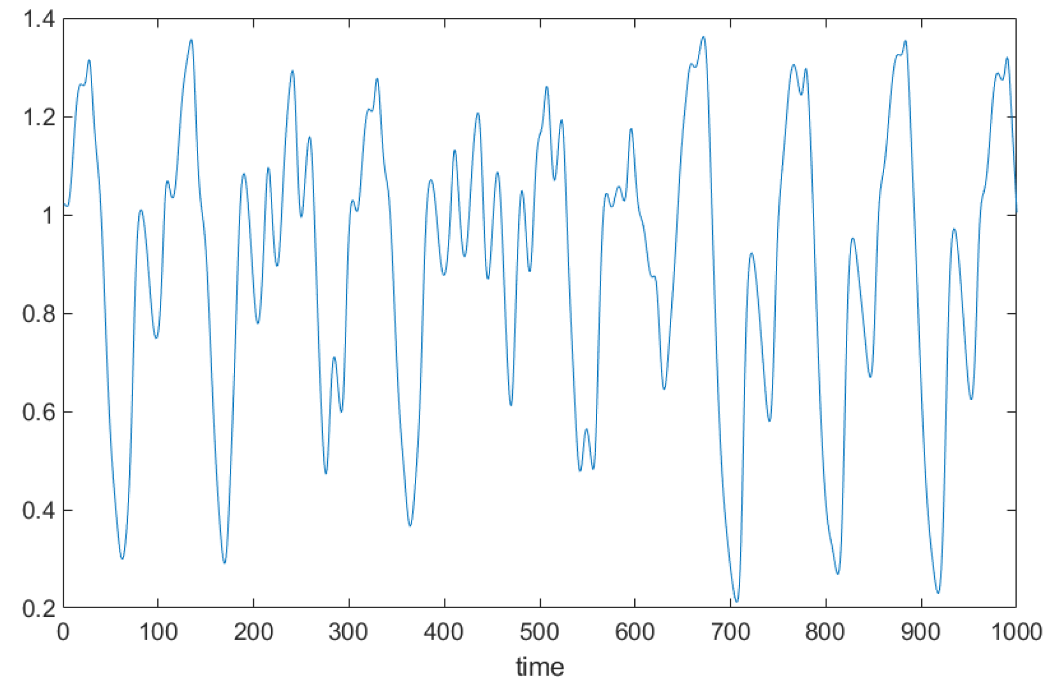
The Mackey-Glass time series prediction is a highly nonlinear regression task, which is widely used as a benchmark problem. The chaotic time series data is generated from the difference equation of the form,

$$\mathit{x}\left(\tau +1\right)=\left(1-b\right)\mathit{x}\left(\tau \right)+a\frac{x\left(\tau -\Delta \tau \right)}{1+\mathit{x}{\left(\tau -\Delta \tau \right)}^{10}},$$

(24)

where we set $a=0.2, b=0.1,$ and $\Delta \tau =30$ in our experiment. Figure 1 shows some part of a generated time series. The input of the neural networks are set as four previous examples in the series, $\mathit{x}\left(\tau \right), \mathit{x}\left(\tau +1\right), \mathit{x}\left(\tau +2\right), \mathit{x}\left(\tau +3\right)$, and the target output is given as the next future value, $\mathit{x}\left(\tau +4\right).$ From the generated time series, we chose 10,000 training samples ($\mathit{x}\left(1001\right)$, …, x (11,000)) and 1000 test samples ($\mathit{x}\left(11,101\right)$, …, x (12,100)).

The network structure for training is the multilayer Perceptrons with 4 inputs, 10 hidden, and 1 output, which is the same as the model used in [21]. Since the output has continuous real values, we adopted the additive Gaussian noise model. Other user-defined parameters for five learning methods are shown in Table 1. Note that we used a larger mini-batch size for SFO in order to ensure its comparable execution time.

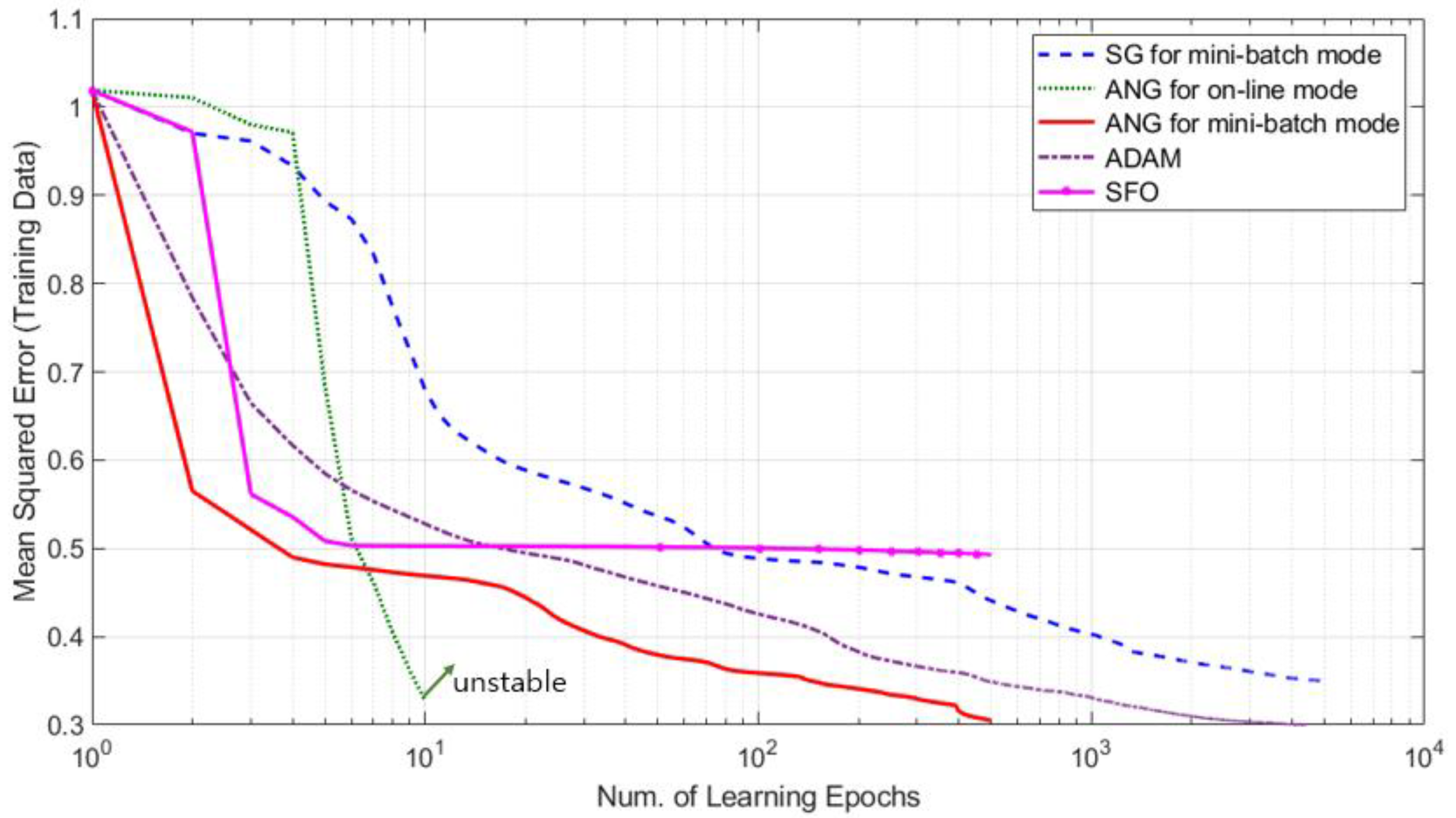
In Figure 2, the changes of training errors of three learning methods according to learning epochs are shown. From the figure, we can see that two adaptive natural gradient methods show better convergence properties than the other three methods. In addition, the proposed mini-batch method gets smaller training error than the conventional online adaptive natural gradient method. Adam optimizer achieved slightly higher training error than the online ANG, but required about 10 times more iterative updates. SFO showed very fast convergence in the early learning stage, but seemed to be trapped at a local minima, giving undesirable solution.

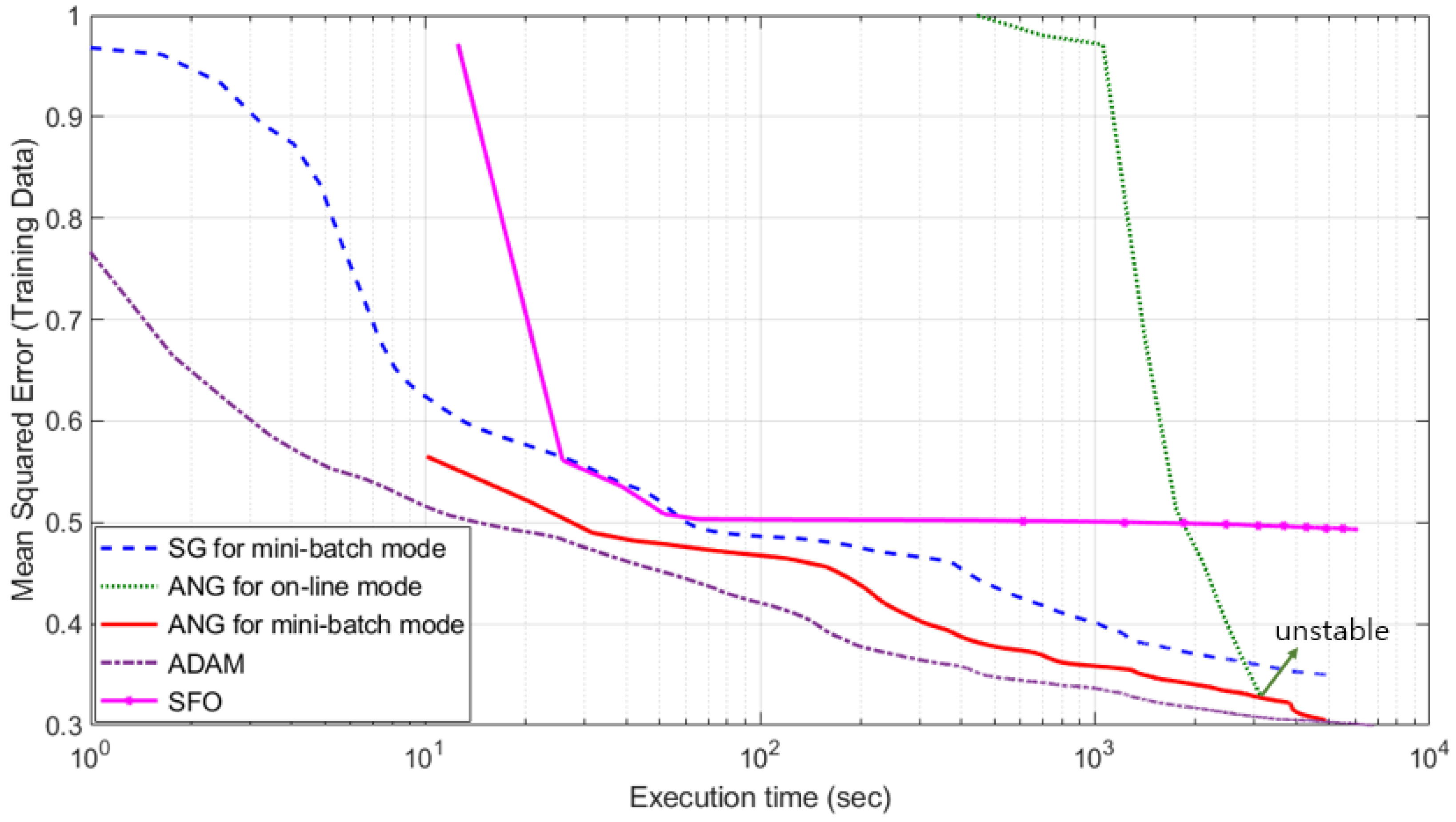
In Table 1, the computational efficiency of three methods are also compared by using the average execution time per single epoch, which shows large differences among the methods. In order to compare computational efficiency and convergence performance at the same time, we plotted the change of errors depending on the execution time (see Figure 3). Note that the horizontal axis of Figure 3 is the execution time in log scale. Form the figure, the superiority of the proposed mini-batch ANG method is confirmed more clearly.

5.3. Experiment for Logistic Regression Model

In order to verify performance of the proposed method for the logistic model, we conducted experiments on the well-known spiral classification data. The task is to classify two dimensional input data scattered in spiral shapes into two classes. Though the network structure was small, it had a highly nonlinear decision boundary as shown in Figure 4, and thus is often used as benchmark data for classifiers. For training, we generated 100,000 samples for each class, (i.e., totally 200,000 samples) as plotted in Figure 4a, and an additional 1000 samples per class for testing (Figure 4b). Whereas the training data can be clearly discriminated by a spiral-shaped decision boundary, there was some overlap in test data, which may cause misclassification.

The network structure is set to 2 inputs, 20 hidden, 2 binary outputs. Other user-defined parameters are given in Table 2. The shape of five learning curves for cross-entropy error depending on the number of epochs is shown in Figure 5. As shown in the figure, the proposed method shows fast convergence compared to the other methods. It should be also remarked that there are large differences in the average execution times for single epoch. Since the online natural gradient need to calculate the natural gradient for each data sample, it takes about 30 times longer execution time than the proposed mini-batch adaptive natural gradient methods. Considering this difference, we also compared the learning curves depending on the execution time, as shown in Figure 6. From the figure, we can confirm the efficiency of the proposed method again. We can also see that Adam optimizer had similar convergence speed to the proposed one in this specific computational environment with a single CPU. Figure 7 shows the decision boundaries that were obtained by three learning methods.

5.4. Experiment for Real Benchmark Data

Finally, we applied the proposed method to a real-world data set, 3D road network data [29], which was obtained from the University of California Irvine (UCI) machine learning repository. The task was to predict highly accurate elevation values for 2D positions given as longitude and latitude. From the whole data set, composed of 434,874 samples, we chose first 300,000 samples for training, and the test was done for the rest (134,874 samples). The network structure is set to 2 inputs, 100 hidden, one output. Since the output has real values, we assumed the additive Gaussian noise model. The values of user-defined parameters are shown in Table 3.

In this real-world data, the number of sample and the number of learning parameters are larger than the previous two simple data sets, and thus the differences in execution time was much bigger, as shown in Table 3. In Figure 8, we showed the change of errors depending on the number of epochs. Note that the horizontal axis is shown in log scale. From the figure, the conventional online natural gradient learning seems to converge fast, though it became unstable after 10 epochs. However, concerning the computational efficiency, the situation was different. In Figure 9, we compared the learning curves depending on the execution time. From the figure, we can say that the proposed method can find a good solution efficiently. Compared to Adam optimizer, the proposed AGN showed about 10 times faster convergence in the sense of learning epochs, but almost the same performance in the sense of execution time. The slow computation may be overcome by using faster matrix multiplication operator.

6. Conclusions

In spite of remarkable developments of deep learning technologies, there is no alternative to gradient-based learning method. The strange learning behaviors of gradient descent learning, such as plateau, local minima, and low generalization error of over-complete models, have not been thoroughly investigated, and the resolution of local minima and plateau problems are still not being fully addressed. Though the original natural gradient has ideal convergence properties eliminating plateau phenomena, heavy computational cost for obtaining the inverse of Fisher information matrix makes the natural gradient unfeasible in real application. As a novel attempt to solve this practical constraint, this paper proposed an explicit and practically implementable algorithm of natural gradient method in mini-batch learning mode. By utilizing mini-batch subsets, we can get computational efficiency as well as estimation stability. In particular, we presented the explicit learning algorithm for two representative stochastic neural network models.

Theoretically, the proposed algorithm does not assume the specific shape of network, and thus is applicable to any types of neural network models trained by gradient descent methods, such as convolutional neural networks and recurrent neural networks. Nevertheless, concerning computational efficiency, we should remark that the popular layer-wise updates through backpropagation process cannot be directly applied to the proposed method because it needs a multiplication of the full rank matrix and the gradient vector for the whole parameters. To overcome this difficulty, it would be possible to combine the proposed method with an additional simplification method for Fisher information matrix such as unit-wise block diagonalization described in [18,30].

Consequently, the proposed algorithm may not be appropriate for deep networks with a huge number of parameters. However, there are diverse applications in which the dimension of input and output is small but its mapping function is highly nonlinear. The proposed method can find a good solution to the problem more efficiently. In particular, in the Internet of Things (IoT) environment streaming huge number of data continuously, the proposed method can be successfully applied to analyze the bunch of data.

References

- Cayamcela, M.E.M.; Lim, W. Artificial Intelligence in 5G Technology: A Survey. In Proceedings of the 2018 International Conference on Information and Communication Technology Convergence (ICTC), Jeju, Korea, 17–19 October 2018; pp. 860–865. [Google Scholar]
- Di Giorgio, A.; Giuseppi, A.; Liberati, F.; Ornatelli, A.; Rabezzano, A.; Celsi, L.R. On the optimization of energy storage system placement for protecting power transmission grids against dynamic load altering attacks. In Proceedings of the 25th Mediterranean Conference on Control and Automation (MED), Valletta, Malta, 3–6 July 2017; pp. 986–992. [Google Scholar]
- Suraci, V.; Celsi, L.R.; Giuseppi, A.; Di Giorgio, A. A distributed wardrop control algorithm for load balancing in smart grids. In Proceedings of the 25th Mediterranean Conference on Control and Automation (MED), Valletta, Malta, 3–6 July 2017; pp. 761–767. [Google Scholar]
- Rumelhart, D.; Hinton, G.E.; Williams, R.J. Learning Internal Representations by Error Backpropagation. In Parallel Distributed Processing: Explorations in the Microstructure of Cognition, 1, Foundations; MIT Press: Cambridge, MA, USA, 1986. [Google Scholar]
- Bengio, Y. Learning Deep Architectures for AI.; Now Publishers: Delft, The Netherlands, 2009. [Google Scholar]
- Hinton, G.E.; Srivastava, N.; Krizhevsky, A.; Sutskever, I.; Salakhutdinov, R.R. Improving Neural Networks by Preventing Co-Adaptation of Feature Detectors. arXiv 2012, arXiv:1207.0580. [Google Scholar]
- Kingma, D.P.; Ba, J.L. ADAM: A method for stochastic optimization. In Proceedings of the International Conference on Learning Representation, San Diego, CA, USA, 7–9 May 2015. [Google Scholar]
- Schraudolph, N.; Yu, J.; Gunter, S. A Stochastic Quasi-Newton Method for Online Convex Optimization. In Proceedings of the Eleventh International Conference on Artificial Intelligence and Statistics; PMLR: London, UK, 2007. [Google Scholar]
- Sohl-Dickstein, J.; Poole, B.; Ganguli, S. Fast large-scale optimization by unifying stochastic gradient and quasi-newton methods. In Proceedings of the 31st International Conference on Machine Learning (ICML-14), Beijing, China, 21–26 June 2014; pp. 604–612. [Google Scholar]
- Andrea, C.; Giovanni, F.; Massimo, R. Novel preconditioners based on quasi-Newton updates for nonlinear conjugate gradient methods. Optim. Lett. 2017, 11, 835–853. [Google Scholar] [CrossRef]
- Al-Baali, M.; Caliciotti, A.; Fasano, G.; Roma, M. Exploiting damped techniques for nonlinear conjugate gradient methods. Math. Methods Oper. Res. 2017, 86, 501–522. [Google Scholar] [CrossRef] [Green Version]
- Caliciotti, A.; Fasano, G.; Roma, M. Preconditioned Nonlinear Conjugate Gradient methods based on a modified secant equation. Appl. Math. Comput. 2018, 318, 196–214. [Google Scholar] [CrossRef]
- Glorot, X.; Bengio, Y. Understanding the Difficulty of Training Deep Feedforward Neural Networks. In Proceedings of the Thirteenth International Conference on Artificial Intelligence and Statistics; PMLR: London, UK, 2010. [Google Scholar]
- Amari, S.-I. Natural Gradient Works Efficiently in Learning. Neural Comput. 1998, 10, 251–276. [Google Scholar] [CrossRef]
- Amari, S.-I.; Park, H.; Ozeki, T. Singularities Affect Dynamics of Learning in Neuromanifolds. Neural Comput. 2006, 18, 1007–1065. [Google Scholar] [CrossRef] [PubMed]
- Park, H.; Inoue, M.; Okada, M. Slow Dynamics Due to Singularities of Hierarchical Learning Machines. Prog. Theor. Phys. Suppl. 2005, 157, 275–279. [Google Scholar] [CrossRef] [Green Version]
- Inoue, M.; Park, H.; Okada, M. On-Line Learning Theory of Soft Committee Machines with Correlated Hidden Units—Steepest Gradient Descent and Natural Gradient Descent. J. Phys. Soc. Jpn. 2003, 72, 805–810. [Google Scholar] [CrossRef]
- Pascanu, R.; Bengio, Y. Revisiting Natural Gradient for Deep Networks. arXiv 2013, arXiv:1301.3584. [Google Scholar]
- Park, H.; Inoue, M.; Okada, M. Slow Dynamics and Singularity in Neural Networks—Standard Gradient vs. Natural Gradient. Lect. Notes Comput. Sci. 2004, 3157, 282–291. [Google Scholar]
- Amari, S.-I.; Park, H.; Fukumizu, K. Adaptive Method of Realizing Natural Gradient Learning for Multilayer Perceptrons. Neural Comput. 2000, 12, 1399–1409. [Google Scholar] [CrossRef] [PubMed]
- Park, H.; Amari, S.-I.; Fukumizu, K. Adaptive natural gradient learning algorithms for various stochastic models. Neural Netw. 2000, 13, 755–764. [Google Scholar] [CrossRef]
- Park, H.; Lee, K. Adaptive Natural Gradient Method for Learning Neural Networks with Large Data Set in Mini-Batch Model. In Proceedings of the 1st International Conference on Artificial Intelligence in Communications, Okinawa, Japan, 11–13 February 2019. [Google Scholar]
- Bottou, L. Online Algorithms and Stochastic Approximations. In Online Learning and Neural Networks; Saad, D., Ed.; Cambridge University Press: Cambridge, UK, 1998. [Google Scholar]
- Goodfellow, I.; Bengio, Y.; Courvill, A. Deep Learning; MIT Press: Cambridge, MA, USA, 2016. [Google Scholar]
- Park, H. Multilayer Perceptron and Natural Gradient Learning. New Gener. Comput. 2006, 24, 79–95. [Google Scholar] [CrossRef]
- Rattray, M.; Saad, D.; Amari, S.-I. Natural Gradient Descent for On-Line Learning. Phys. Rev. Lett. 1998, 81, 5461–5464. [Google Scholar] [CrossRef]
- Wei, W.G.H.; Liu, T.; Song, A.; Zhang, K. An adaptive natural gradient method with adaptive step size in multilayer perceptrons. In Proceedings of the 2017 Chinese Automation Congress (CAC), Jinan, China, 20–22 October 2017; pp. 1593–1597. [Google Scholar]
- Petersen, K.B.; Pedersen, M.S. The Matrix Cookbook; Technical University of Denmark: Copenhagen, Denmark, 2012. [Google Scholar]
- Guo, C.; Ma, Y.; Yang, B.; Jensen, C.S.; Kaul, M. EcoMark: Evaluation Models of Vehicular Environmental Impact. In Proceedings of the 20th International Conference on Advances in Geographic Information Systems; ACM: Redondo Beach, CA, USA, 2012. [Google Scholar]
- Ollivier, Y. Riemannian metrics for neural networks, I: Feedforward networks. Inf. Inference 2015, 4, 108–153. [Google Scholar] [CrossRef]
Figure 1.
Mackey-Glass time series data (test samples).
Figure 2.
Change of prediction errors for Mackey-Glass series depending on the number of epochs.
Figure 3.
Change of prediction errors for Mackey-Glass series depending on the execution time.
Figure 4.
Spiral data sets: (a) Training data samples and (b) test data samples.
Figure 5.
Change of errors for spiral data classification depending on the number of epochs.
Figure 6.
Change of errors for spiral data classification depending on the execution time.
Figure 7.
Obtained decision boundary by (a) standard gradient (SG), (b) online adaptive natural gradient (ANG), (c) proposed mini-batch ANG, (d) Adam optimizer, and (e) sum of functions optimizer (SFO).
Figure 8.
Change of errors for evaluation prediction depending on the number of epochs.
Figure 9.
Change of errors for evaluation prediction depending on the execution time.