Crack Initiation and Propagation Fatigue Life of Ultra High-Strength Steel Butt Joints


1
Chair of Mechanical Engineering, Montanuniversität Leoben, Franz-Josef-Straße 18, 8700 Leoben, Austria
2
voestalpine Stahl GmbH, voestalpine-Straße 3, 4020 Linz, Austria
*
Author to whom correspondence should be addressed.
Appl. Sci. 2019, 9(21), 4590; https://doi.org/10.3390/app9214590
Submission received: 31 August 2019
/
Revised: 12 October 2019
/
Accepted: 13 October 2019
/
Published: 29 October 2019
(This article belongs to the Special Issue Recent Trends in Advanced High-Strength Steels)
Abstract
:The division of the total fatigue life into different stages such as crack initiation and propagation is an important issue in regard to an improved fatigue assessment especially for high-strength welded joints. The transition between these stages is fluent, whereas the threshold between the two phases is referred to as technical crack initiation. This work presents a procedure to track crack initiation and propagation during fatigue tests of ultra high-strength steel welded joints. The method utilizes digital image correlation to calculate a distortion field of the specimens’ surface enabling the identification and measurement of cracks along the weld toe arising during the fatigue test. Hence, technical crack initiation of each specimen can be derived. An evaluation for ten ultra high-strength steel butt joints reveals, that for this superior strength steel grade more than 50% of fatigue life is spent up to a crack depth of 0.5 mm, which can be defined as initial crack. Furthermore, a notch-stress based fatigue assessment of these specimens considering the actual weld topography and crack initiation and propagation phase is performed. The results point out that two phase models considering both phases enable an increased accuracy of service life assessment.
1. Introduction
1.1. Fatigue Assessment of Welds Considering Crack Initiation and Propagation
The fatigue life of a component is a very complex physical process which could be divided to five stages [1]: dislocation movement, crack nucleation, micro- and macro crack propagation and the final fracture. For fatigue assessments of welded joints, the individual consideration of each phase is usually too complicated. Most procedures focus on the stages up to a crack of detectable size. Fracture mechanical approaches, on the other hand, neglect all stages before macro crack propagation. In order to increase the accuracy of technical fatigue assessments, two-phase models considering both crack initiation and propagation are introduced [2]. Hereby, the first three stages are treated as the crack initiation phase (index init) followed by a crack propagation phase (index cp). Thus, the total fatigue life up to burst fracture Nf sums up the cycles of both phases Ninit and Ncp, respectively. The transition between these two phases is referred to as technical crack initiation at a crack depth ath; its value varies depending on the selected model [3,4,5,6]. In the literature, various approaches exist for an assessment of the crack initiation phase, such as the fatigue notch factor Kf [7,8,9], strain life approaches [10,11] or the notch stress intensity factor [12,13]. The crack propagation phase, on the other hand, is generally assessed using linear elastic fracture mechanics.
1.2. Detection of the Crack Initiation Point
The result of a standard load controlled fatigue test is the number of load cycles until burst fracture at a certain load level, including the crack initiation and propagation phase. For cylindrical small-scale specimens without considerable imperfections, such as pores, the crack propagation phase is rather small compared to crack initiation. Therefore, the S-N curves obtained by such standard tests could be applied in fatigue life assessment concepts to estimate the time to crack initiation [14]. For welded components, on the other hand, the specimens should exhibit a certain width/sheet thickness ratio in order to ensure a steady state residual stress state and crack initiation from a plain weld rather than the specimen’s edges [15]. In practice, a minimum width of three to five times the sheet thickness is suggested to avoid such effects [16,17] causing welded specimens to be comparably large even in the case of thin sheets. Therefore, the crack propagation life of welds significantly contributes to the specimen’s total fatigue life [18,19,20]. Hence, the knowledge about the technical crack initiation enables a split of the fatigue assessment to crack initiation and crack propagation phases. This is of great interest even for fatigue tests of welded specimens, as it makes a more precise assessment of a structure’s fatigue life possible.
A number of different methods exist for monitoring crack propagation. For welded structures, local strain measurement at hot spots [21,22] is widely used due to its flexibility and easy handling. This procedure is expedient if the specimen has a low number of distinct hot spots, such as a longitudinal stiffener, where crack initiation will occur. Otherwise, a high number of strain gauges is necessary to cover the whole highly-stressed weld toe area.
Another common technique is the application of a mixture of zinc oxide and glycerine on the weld toe [21,23] giving a colour change from white to black when a crack initiates. The main disadvantage of this method lies in the fact that the weld is covered by a viscous fluid preventing any exchange of oxygen leading to a possible change of crack initiation and propagation behaviour.
A purely optical tracking of crack propagation is performed in [24,25]. Hereby, an industrial camera tracks the crack’s surface extension using its contrast to the surrounding surface. This procedure achieves high accuracy but it requires a fine surface quality and special lighting.
In [24], the optical tracking is compared to the crack propagation detected via crack gauges. For this procedure, a crack gauge is applied on the surface region where the crack is expected. During the fatigue test, constant current flows through the crack and the resistance based on voltage drop is measured. As the crack opens, the crack gauge is torn apart, thereby increasing the resistance of the gauge, which can be linked to the surface crack length. The comparison between optical measurement and crack gauges in [24] reveals a sound accordance.
The eddy current method applied in [26,27] enables non-contact measurement of surface cracks even below paint coatings. Thereby, eddy currents proportional to the conductivity of the material are induced by placing an AC-energized probe coil near the surface of the specimen. Discontinuities, such as cracks, affect the magnitude and phase of the induced current. The consequential magnetic field is then sensed by the probe indicating the presence and size of the surface crack.
Digital image correlation (DIC) is used for estimating stress intensity factors in [28] and the consequential identification of crack propagation law parameters in [29]. In [30], DIC and crack opening displacement techniques are combined to monitor crack propagation tests. Therewith, the fatigue behaviour of thin cracked plates made of aluminium alloy in crack propagation mode I are analysed.
1.3. Effect of Local Weld Geometry on Fatigue Performance
Modern welding technologies involving highly automated processes enable the production of high-quality welds exhibiting a very smooth transition at the weld toe. Nevertheless, variations in weld geometry due to the dynamic welding processes cannot be eliminated entirely. These very local discontinuities often govern the fatigue performance of welds due to its locally pronounced notch effects. Due to the increasing demands on quality of the welds of high-strength structural components, the effect of local weld geometry on the fatigue performance is of particular relevancy. Therefore, an assessment of such variations is essential in order to determine the maximum allowable size and extension.
In [31,32,33], the linear elastic stress concentration factor is utilized to take weld geometry into account. Thereby, Ref. [31,32] determine the stress concentration factor by the aid of linear elastic FE-analysis, whereas [33] uses analytical equations. In general, this procedure is prone to overestimating the effect of the actual geometry, as support effects are not considered. However, a local fatigue notch factor can be obtained by evaluating the local notch stress course, the stress gradient and, finally, the corresponding supporting factor [34].
Radaj proposed to replace the actual weld toe transition radius by a fictitious radius ρf in order to take support effects into account [9] (see Equation (1)). In [33], this procedure leads to better matching results than the use of the actual transition radius.
The effective notch stress concept [9,35,36,37] proposes a reference notch radius of ρref = 1 mm independent of the actual geometry. Thereby, a crack-like weld toe exhibiting an actual weld toe radius of ρ = 0 mm is assumed leading to a fictitious radius ρf =ρref = 1 mm in Equation (1). This concept is part of the International Institute of Welding (IIW) guideline [38], verified and consistent for structural steels and aluminium alloys. However, it does not consider the actual weld toe geometry. Therefore, it tends to deliver conservative results especially for high-quality high-strength welds with extremely shallow weld toes.
In [39], the critical distance approach developed by Lawrence [10] is applied. Thereby, the fatigue notch factor Kf is calculated from the stress concentration factor Kt using the Peterson formula. The required parameter a*, the critical distance, is related to the ultimate tensile strength of the material.
Neuber proposed in [8] an evaluation method based on stress averaging in order to consider microstructural support. Hereby, the fatigue assessment is performed using an effective stress σeff obtained by averaging of the stress distribution in depth σ(x) over the microstructural support length ρ* at the surface layer instead of the linear elastic stress maximum (see Equation (2)). The fraction of σeff and the nominal stress σn gives the fatigue relevant effective stress concentration factor Kf (see Equation (3)).
Values for the key parameter ρ* are provided by Neuber himself for various materials in [8]. For welded structural steels exhibiting a microstructure similar to steel castings a microstructural support length of ρ* = 0.4 mm is suggested leading to the effective notch stress concept with a fictitious transition radius of ρref = 1 mm, which is mentioned above in Radaj’s concept. In [40], comprehensive investigations on the effect of weld geometry on the fatigue strength under consideration of the microstructural support length are published. Here, a significantly smaller microstructural support length of around ρ = 0.1 mm reveals the lowest scatter band of all fatigue test results. This is traced back to the high hardness of the weld, where Neuber’s initial suggestion for ferritic steel is more appropriate instead of cast steel.
In many cases, the effects of the weld geometry regarding to fatigue strength is assessed using fracture mechanics neglecting the crack initiation phase. In [41], the effects of variations of weld geometry parameters are studied systematically. A comparison to test results reveals the best agreement using a semi-elliptical crack with an initial depth of ainit = 0.05 mm. The work published in [42] presents a holistic study on the effects of the weld geometry applying the IBESS-model [43], a fracture mechanics-based prediction of the fatigue strength of welded joints. Mashiri et al. [44] carried out crack propagation analysis using the boundary element analysis. Their investigations on the effect of weld profile and undercuts on fatigue life shows the best fit at an initial crack length of ainit = 0.1 mm. In [45,46], the Frost diagram is utilized to assess undercuts from a fracture mechanical perspective. The focus hereby lies in the establishment of undercut tolerances for industry.
Concluding, numerous local approaches are currently available for fatigue assessment of welded joints, but for calculation one has to apply proper local weld toe geometry values especially in the case of high-quality welds.
2. Experimental Investigations
The experimental work of which results are utilized in this paper, especially specimen manufacturing and details regarding the fatigue testing setup, have been already published in [47]. This chapter provides a short overview on the invoked test procedure for completion. In addition, investigations on the crack propagation parameters of the weld’s base material are performed and described in this section.
2.1. Fatigue Tests
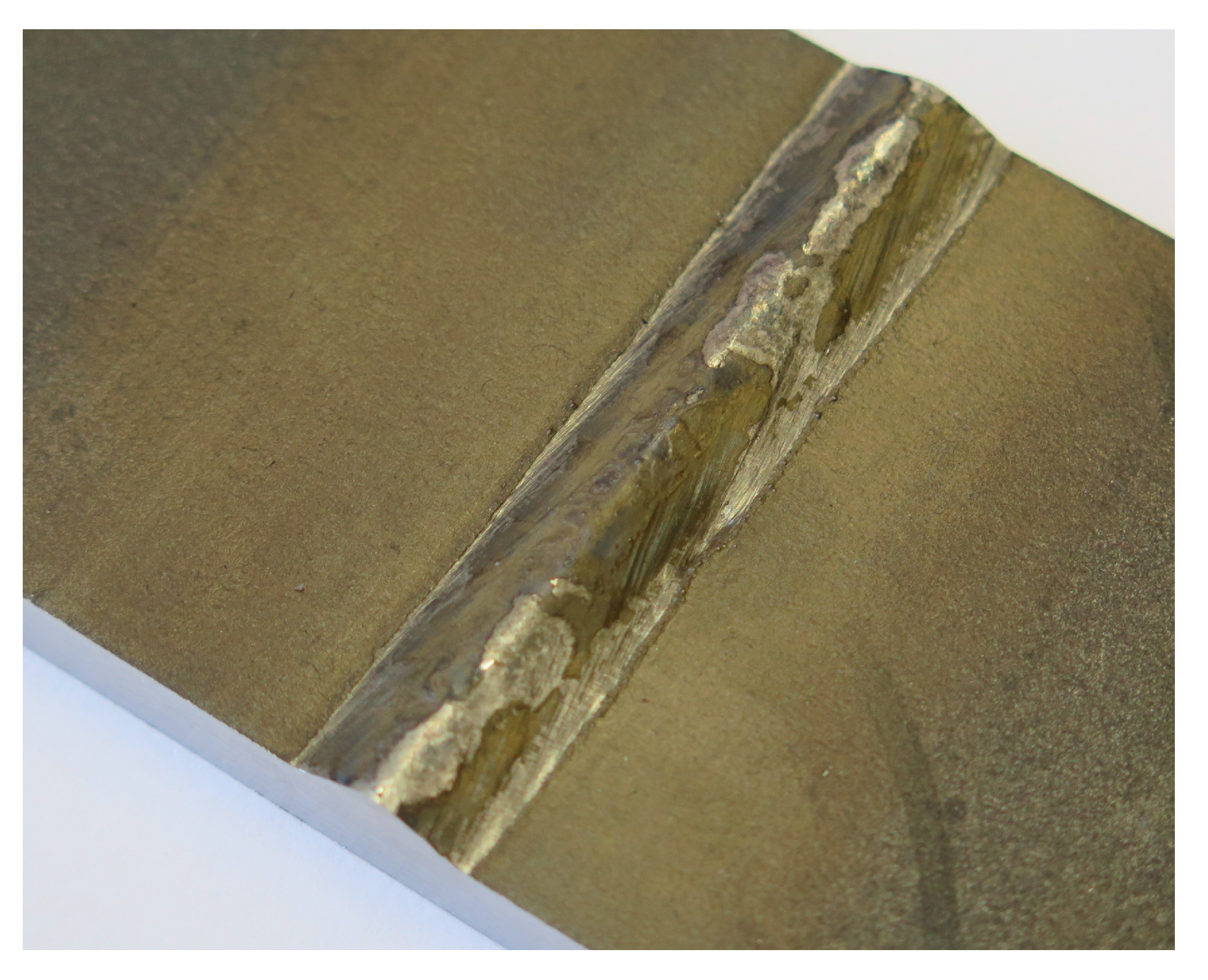
The two-layer butt-welded specimens are manufactured using S1100 base material of 6 mm sheet thickness, T89 metal core filler wire and standard M21 shielding gas. The mechanical properties of the base and filler metal are listed in Table 1. An optical inspection of the specimens after the manufacturing process reveals undercuts at the weld toe of several specimens (see Figure 1). These specimens undergo a surface topography scan prior to fatigue testing in order to investigate the effect of these imperfections. The tumescent tensile fatigue tests were carried out under standard atmosphere at a stress ratio of R = 0.1 and a test frequency of f = 10 Hz up to burst fracture or a run-out level of 10 million load cycles. The statistical evaluation in finite life regime is performed according to [48] using arbitrary slope values, whereas the run-out level is assessed by the arcsin√P-procedure [49] with a decrease of 10% per decade in fatigue strength corresponding to a slope of k = 22, as suggested in [50]. Figure 2 shows the fatigue test result, where the effect of the weld undercuts regarding to fatigue strength is clearly visible. However, in some cases the reduction in fatigue life is far less pronounced than expected based on the evaluation of each weld’s stress concentration factor (see Section 4.1 and [47,51]). Figure 3 shows the fracture surface of a defective specimen clearly identifying the crack initiation point at the undercut.
2.2. Determination of Crack Propagation Parameters
The assessment of crack propagation life requires the knowledge of suitable material parameters describing the crack propagation behaviour. Therefore, the determination procedure utilizing crack gauges presented in [24] is applied to measure the crack propagation of S1100 base material exhibiting 6 mm sheet thickness. Hereby, four single edge notch tension (SENT) specimens are tested under constant amplitudes at a stress ratio of R = 0.1 recording the respective crack propagation. The subsequent evaluation of the fatigue crack growth rate is performed according to ASTM E647 [52]; the according geometry factor to determine the specimens stress intensity factor is based on [53]. Figure 4 shows the resulting long-crack propagation behaviour of all four specimens.
In the literature, many different models are provided describing the materials’ behaviour in the da/dN—ΔK regime; for example, in [54,55]. For this work, the crack propagation model according to Paris-Erdogan [56] is applied requiring only two parameters CP and mP (see Equation (4)). A non-linear fitting procedure was used to determine these parameters for the present experimental data, whose result is plotted in Figure 4 as well. The consequential values are CP = 8.3509×10⁻¹⁰ and mP = 1.721 for units of mm/cycle and MPa√mm, respectively.
3. Optical Detection of Crack Initiation and Propagation
The following section presents an engineering feasible method for detecting crack initiation and tracking its propagation of welded specimens. This quite straightforward procedure is based on digital image correlation of pictures of the specimens acquired during the experiment using a common single-lense reflex (SLR) camera system.
3.1. Experimental Setup
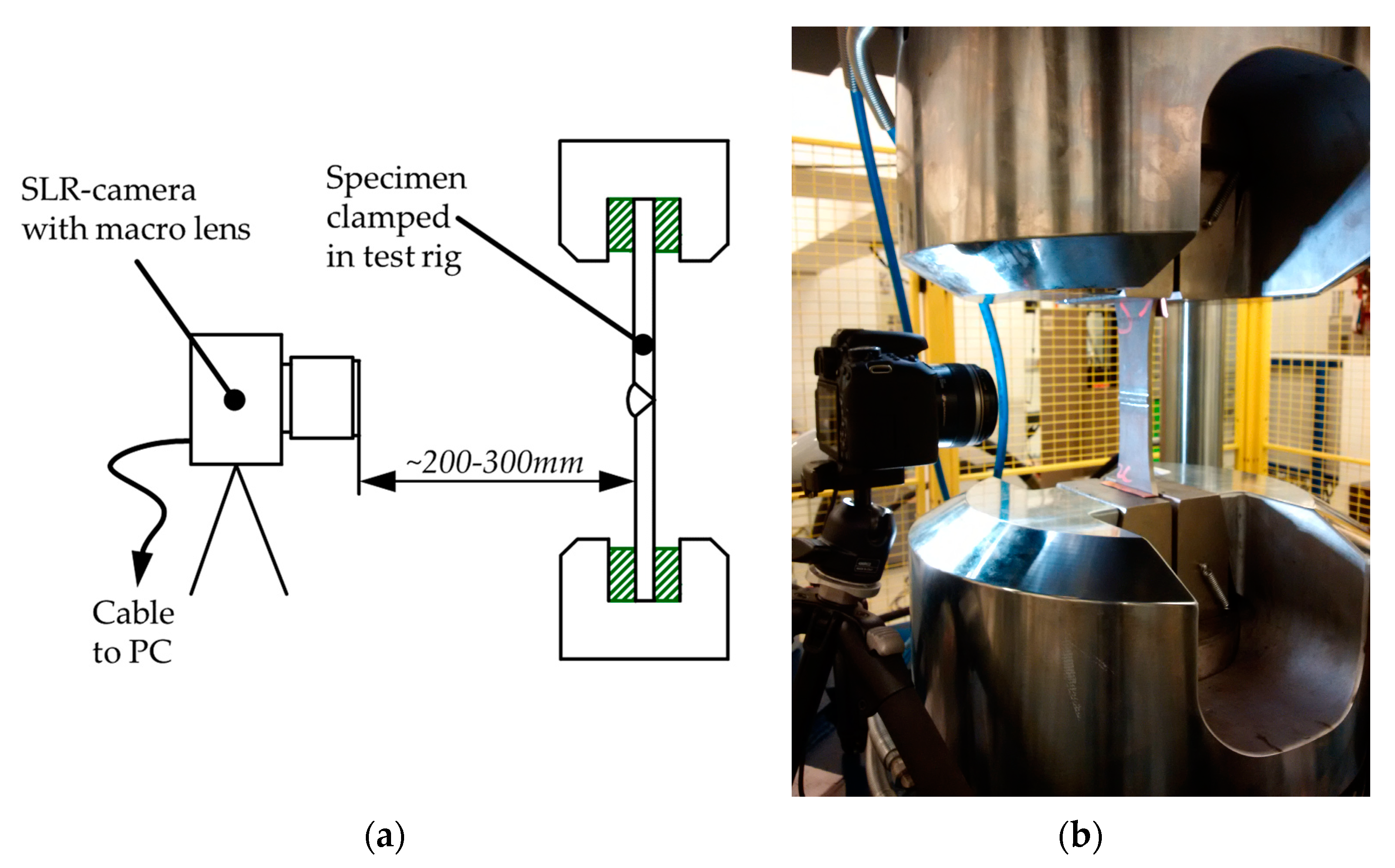
The setup for this method is very simple and does not require any changes on the specimen itself (see Figure 5). A common digital SLR camera is placed around 20–30 cm off the specimen’s surface. The exact distance is figured out empirically for each specimen type in order to fit the region of interest to the camera’s captured area and its focus settings. In order to trigger the camera during the fatigue test, the cameras trigger button is connected to the control computer for the hydraulic test rig. The applied camera is a Canon (Ōta, Tokyo, Japan) EOS 650D featuring a comparably high resolution of 18 megapixels. The lens selected for the pictures is a Canon EF-S 60mm f/2.8 Macro USM macro lens enabling a detailed view of the region of interest without the risk of collision with the clamping devices. A lighting system consisting of an LED lamp is installed to ensure lighting independent of the time of day.
The image acquisition is performed at the specimens’ upper load Fu causing possible cracks to open. Before running the test, a reference image is taken at maximum loading as a basis of comparison, which is required by the subsequent post-testing digital image correlation procedure. At first, the possibility of synchronized image acquisition during fatigue testing was checked. However, as the image has to be taken exactly at the maximum load, a very short shutter time is required in order to ensure a clear picture with adverse impact on the image quality. Hence, the run cycle of the fatigue test stops at maximum load for the image acquisition for a few seconds (see Figure 6). Due to the short retention time and standard conditions around the specimen, holding the specimen at maximum load does not affect the crack initiation and propagation behaviour.
The image acquisition starts with a reference image before test start and continues after a certain number of load cycles Ninitial. This initial cycle number is based on previous tests and strongly depends on the load level of the respective test. The a priori fatigue testing reference image and the image taken at the initial cycle number show no distinct difference, implying early-stage crack propagation. After the initial image acquisition, the fatigue test is continued block by block. The number of load cycles between two images Ninterval increases with the load cycle number according to Table 2. Both measures reduce the number of images to be taken without a significant decrease of the procedure’s accuracy. A final image of the broken specimen at Nf provides insight on the failure-tripping crack in case of several initiated cracks.
3.2. Crack Detection and Tracking Procedure
A Matlab©-based procedure (R2017b, The Mathworks, Inc.; Natick, Massachusetts, USA) is developed for detection of crack initiation and subsequent tracking of crack propagation. Essentially, it is divided into two sections. At first, digital image correlation is applied to the acquired images in order to get a local distortion field of the specimen’s surface. Therefore, an algorithm submitted to Matlab Central File Exchange by Elizabeth Jones [57] (File ID #43073) provides the basic functions. This code is evaluated using standard test images by the Society for Experimental Mechanics (SEM) in the DIC-Challenge, see [58] and the website https://sem.org/dic-challenge/. The second section detects crack initiation and tracks crack propagation using the distortion field gathered in the first step.
The procedure’s structure and operation is described in the following subsection using exemplarily a specimen tested at a nominal stress range of Δσn = 400 MPa, an image acquisition after Ninitial = 60,000 load cycles and Nf = 85,039 load cycles until burst fracture.
3.2.1. Local Distortion Field of the Specimen’s Surface
A crack in a structure leads to a local reduction of the stiffness along with a significant increase of local displacement in case of a load perpendicular to the crack surface. Therefore, the change in local displacement is a suitable parameter for the detection of surface cracks. Hereby, digital image correlation is an appropriate tool in order to measure this parameter using the images acquired during the fatigue tests. Digital image correlation is a camera-based toolbox to acquire full field displacements by cross-correlation. Usually, speckle patterns are applied to the measured surface in order to increase the surface contrast. However, in the present case the texture of the specimens’ surface itself turned out to be sufficient for correlation in the desired regions. This is a great advantage compared to other crack detection methods as any surface modification could lead to a change in the weld’s crack initiation and propagation behaviour.
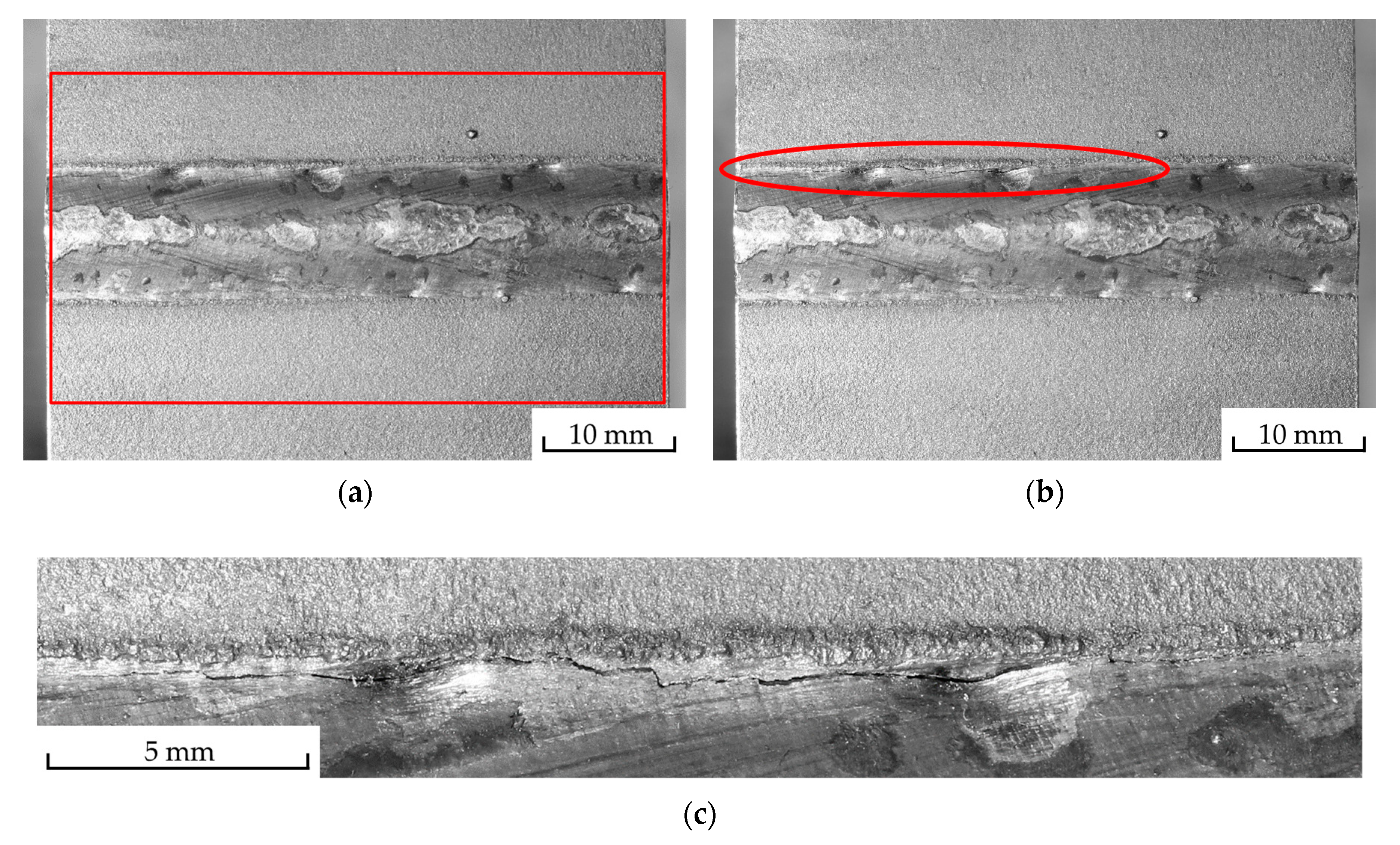
The image correlation procedure compares each image at a certain number of load cycles with the reference image acquired at the beginning of the fatigue test. In order to exclude any effects coming from optical distortion due to the camera lens, the Matlab© built-in Camera Calibrator is applied to estimate the geometric parameters of the utilized lens. Subsequently, the distortion effects are removed of the acquired images. Figure 7 shows the grayscale images prepared for image correlation of Reference (a) and last image (b) of the exemplary specimen. Here, the x-axis corresponds to the horizontal and the y-axis to vertical direction. The last image already shows a large crack at the upper weld toe leading close to burst fracture. However, the actual size of the crack is not visible. In order to increase the correlation speed, parts of the image are excluded from correlation which do not contain relevant information, such as the areas to the left and right of the specimen. Here, Figure 7a shows the processed net surface as a red rectangle. The correlation procedure requires a set of parameters affecting its quality and accuracy as well as the calculation time which are described in the documentation of the code (see [59]). Hereby, a suitable set of parameters for the current images is invoked using the documented approach and further empirical investigations. One of the most sensitive parameters is the grid spacing defining the distance in pixels between two adjacent control points. At these points, the output distortion is computed. Therefore, the grid spacing represents the resolution quality of the result directly linked to computation time. For example, an image with a size of 6000 × 4000 pixels and a grid spacing of 15 pixels results in a distortion field of 400 × 267 entries. Here, a large grid spacing gives a rather coarse distortion field whereas a fine grid spacing leads to a disproportional long calculation time of several hours per image and increases the risk of poor correlation results. Thus, a grid spacing between 15 and 20 pixels is recommended. A more detailed insight on the correlation procedure and its parameters is given in [60].
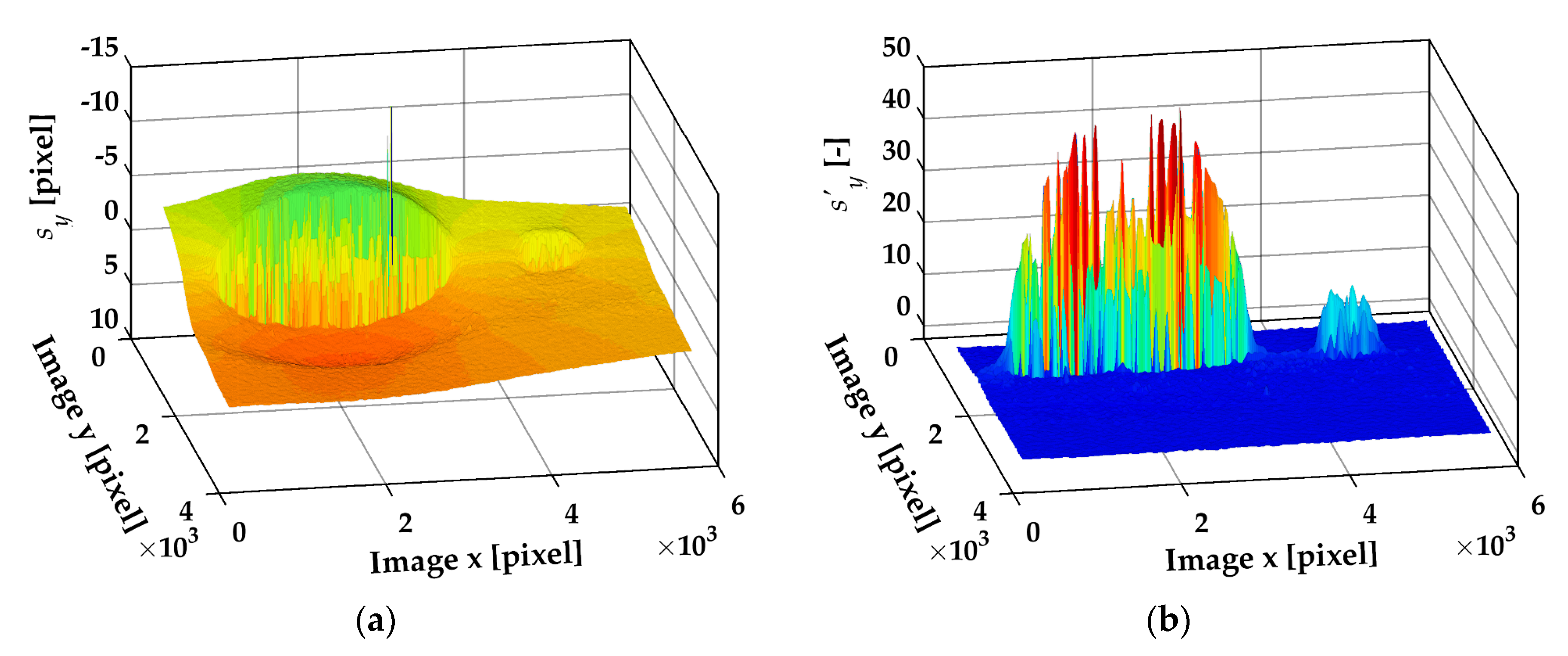
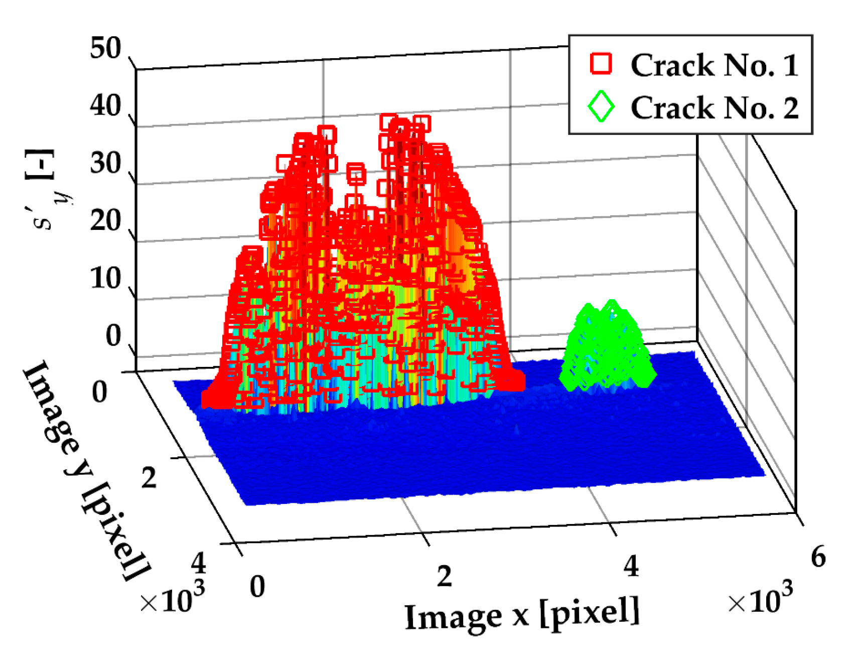
The result of the image correlation procedure for N = 84,000 is depicted in Figure 8a as the vertical displacement field sy in the load direction of the specimen. This outcome includes the local displacement as well as a potential global movement of the specimen due to a small amount of sliding in the clamping area. Therefore, the vertical gradient of the vertical displacement s’y is introduced in order to highlight local changes in vertical displacement and simultaneously exclude possible global movement. The corresponding result of the displacement gradient is depicted in Figure 8b explicitly indicating the present cracks only.
3.2.2. Crack Detection and Tracking
This section deals with the identification of a crack and its tracing over the load cycle number based on the results of the digital image correlation procedure. This includes recognition of a newly initiated crack to an existing one, as well as the merging of two small cracks into a larger one. This part of the procedure is once again divided into two subsections; the first covers the detection of all cracks for each image separately. The second traces the growth with increasing load cycle number and determines possible merges, as well as initiation of new cracks.
The identification of cracks in an image is performed utilizing the Matlab implemented image processing toolbox. Therefore, the gradient field is converted to a binary black-white image with an initial threshold value s’y,thres of two pixels/pixel. If the maximum gradient value of an image exceeds forty pixels/pixel, the threshold value is adapted to five percent of the maximum value. The reason for this lies in the enlargement of the plastic zone at the crack tip with increasing crack length [55], which is considered by this adaptive threshold setting. It has to be noted that the definition and the course of the threshold value is, besides the parameters of the image correlation, the primary influencing factor regarding the finally-measured crack length. Therefore, it plays a decisive role in the procedure’s verification process (see Section 3.3.). Figure 9 shows the black-white image related to Figure 8b with a threshold value of s’y,thres = 2.39. Figure 10 plots the result of crack identification process in the gradient field of Figure 8b.
Based on the results of each image, crack tracking is performed over all of the images. At first, the last image before fracture is considered by identifying the number and positions of the final cracks before specimen failure. This information is essential, as all crack initiations will occur in these areas. However, due to this action, the procedure is not suitable for application during the test without any modification. Subsequently, a loop through all images assigns the respective cracks to a final crack. Additionally, the merging of cracks is noted at this point by a comparison to the previous image’s state. Finally, the determined surface crack length is converted from pixels to millimetres.
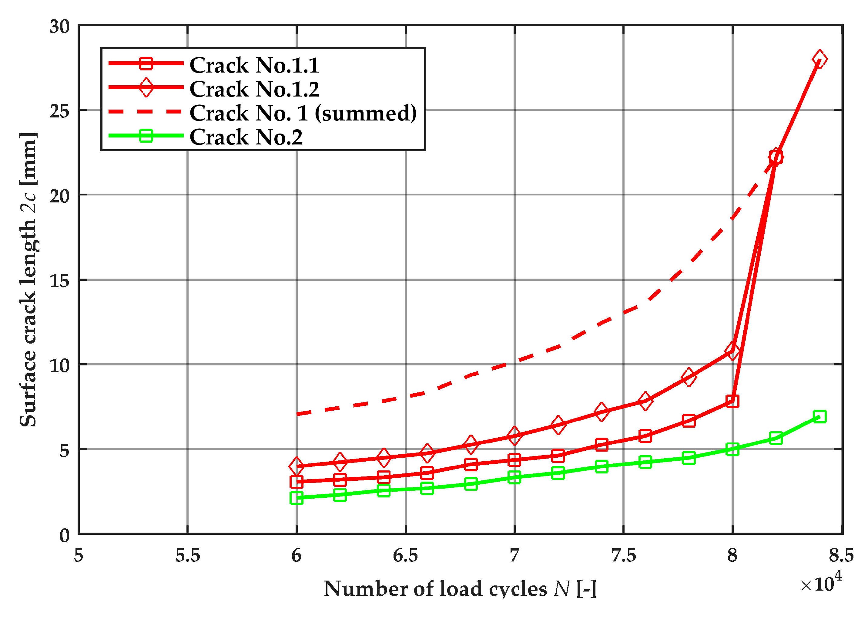
Figure 11 shows the procedures result, the surface crack length 2c in mm with respect to the load cycle number. Crack number one actually initiated at two different positions and merged just a few thousand load cycles before final fracture. Figure 12a shows the image of the first step at 60,000 load cycles with marked crack number one in red and two in green dye. In this picture, the two separate initiations of crack one are visible, which will merge within further crack growth. Figure 12b depicts the image of the last step before fracture at 84,000 load cycles where crack one is already merged. The respective fracture surface after 85,039 load cycles in Figure 12c gives a good opportunity to verify the result. Here, the two initiation points within the left crack are clearly visible. Furthermore, all three crack initiation points are located at local undercuts, which are indicated in the figure.
3.3. Validation of the Procedure
The procedure for crack detection and tracking presented in this section is based on estimations and parameters, which are assessed empirically. Therefore, the procedure requires a validation process in order to prove, that the assessed crack length is properly evaluated. This is of importance, as the result not only includes the presence of a crack but also provides the absolute surface crack length value in millimetres.
Two different approaches are used for validation. The first, more comprehensive test includes block load testing of a notched specimen in order to create beach marks at the fracture surface, which can be easily compared to the procedures result. The second approach is based on fracture surfaces of welded specimens exhibiting a second not through-crack, whose measurements can be compared to the procedure’s results as well.
3.3.1. Beach Marks
The first validation approach utilizes beach marks at a fracture surface as basis for comparison. Therefore, a block load fatigue test is performed using a notched specimen made of 10 mm S355 construction steel. The spark-eroded semi-elliptical notch placed at the centre of the 40 mm wide specimen exhibits a depth of 1 mm and a surface length of 2.5 mm and acts as initial crack. The block load test consists of alternating sequences of 20,000 load cycles at an upper level Δσ = 250 MPa and a lower level of Δσ = 150 MPa at a constant stress ratio of R = 0.1. Therefore, crack propagation rates vary for each block, which appears at the fracture surface. Further details on specimen geometry and experimental procedure are given in [61]. During fatigue testing, an image is acquired every 5000 load cycles corresponding to a number of four images per block.
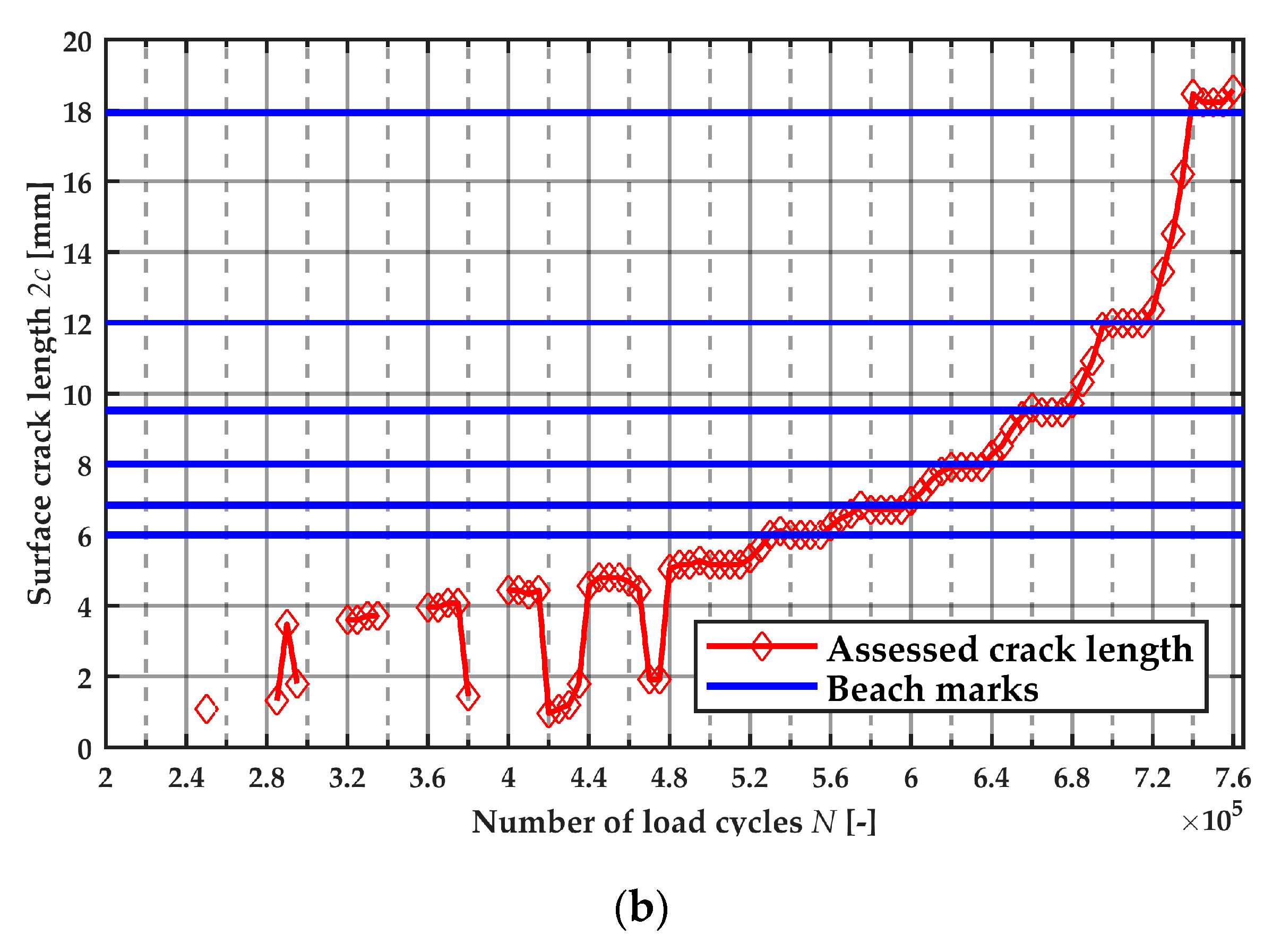
After the fatigue test, a high-resolution image of the fracture surface is acquired. In total, six beach marks have enough contrast to ensure a reliable measurement. Figure 13a shows the fracture surface of the block load test including the measurement results. The result of the crack detection and tracking procedure is plotted in Figure 13b; additionally, the measurement results are shown as horizontal lines. Table 3 shows the according numbers including the percentage difference. The comparison between measurement and assessment leads to very satisfactory results, the deviation for all assessed beach marks is less than two percent. This confirms the set of parameters used for the image correlation and crack detection procedure.
At this point it should be noted that the crack propagation of this specimen starts at both ends of the semi-elliptical notch nearly at the same load cycle number. Especially during low load blocks, the procedure detects these two cracks separately, neglecting the presence of the notch in between. Therefore, the assessed surface crack length in such cases is about the surface length of the notch smaller than the total tip to tip length. This explains the behaviour of the surface crack length trace in Figure 13b jumping up to a load cycle number of 480,000.
3.3.2. Fracture Surfaces
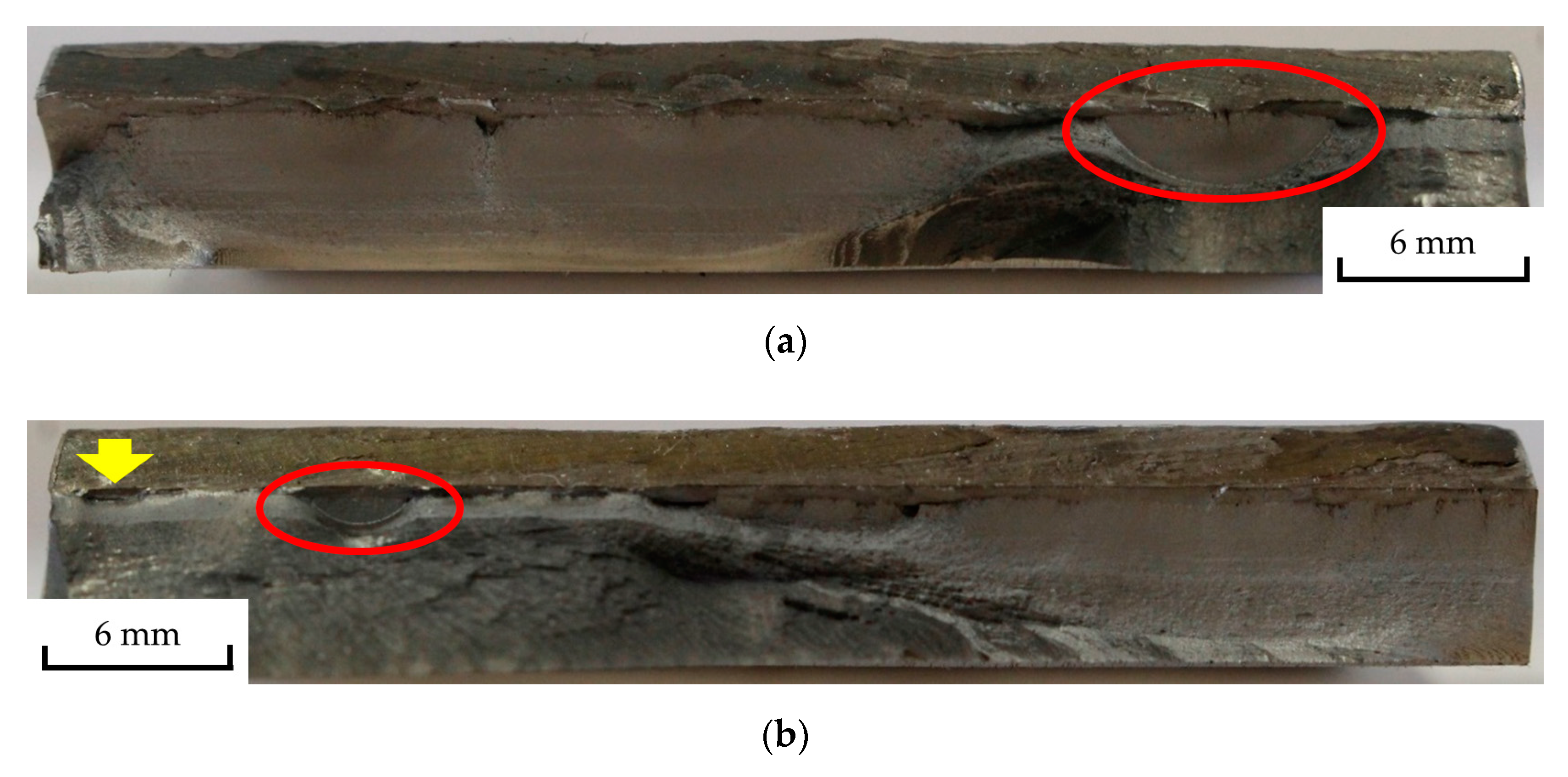
The second part of the method’s validation utilizes separate, not-through base plate thickness cracks in the fracture surface. The fracture-causing crack itself is not suitable for a comparison with the calculated value, as the transition zone from stable crack propagation to rupture is vague. This inhibits a precise measurement of the final surface crack length. The number of such separated, not-through cracks is limited and takes place preferably in high load levels, where the tendency for multi-crack initiation is higher. However, two suitable fracture surfaces are available for validation within the present test series (see Figure 14).
The measurement of the actual crack length in the fracture surface is performed utilizing a Matlab©-tool introduced in [25]. The script fits a semi-ellipse to a number of points manually selected in the image using a non-linear fitting algorithm. Figure 15 displays the result of the fitting procedure for both specimens including the crack measures. Hereby, the shape of the crack in Figure 15a fits the semi-ellipse quite well, whereas the smaller crack in Figure 15b deviates from the semi-elliptical shape considerably. However, the surface length is assessed properly.
Due to the strategy of the presented crack detection procedure, the measurement of the surface crack length cannot be performed at burst fracture. Thus, quadratic extrapolation from the last four measurement results up to the number of load cycles at burst fracture is performed. This assumption could lead to an underestimation of the actual crack length. However, it delivers sufficient accuracy and does not require any local material parameters affecting the extrapolation.
Table 4 presents the calculated surface crack length with respect to load cycle numbers for both investigated cracks including the extrapolated values at burst fracture. The measured values originating from the fracture surface are listed as well for direct comparison. Hereby, the actual surface crack length exceeds the extrapolated values of about 2% in both cases. This, once more, validates the approach and the determined parameters of the crack detection and tracking procedure.
4. Fatigue Assessment
This section assesses the fatigue life of welded ultra high-strength steel butt joints and evaluates the effect of undercuts.
4.1. Neuber’s Stress Averaging Method
The stress averaging method proposed by Neuber utilizes the microstructural support length ρ* in regard to microstructural support. As already stated in Section 1, suggestions for this parameter often deviate from determinations using the lowest scatter-band of the resultant S-N curve as a key factor, especially in the case of welded specimens.
The local stress distribution at the weld toe and its trace in depth is well known due to surface topology scans and subsequent numerical analysis of this geometry of all ten specimens (see [47,51]). The values for the effective stress σeff(ρ*) and the corresponding fatigue notch factor Kf(ρ*) are calculated for each specimen at the respective points of crack initiation. The required stress distribution in depth σ(x) is taken from the numerical analysis of the actual specimen’s weld topography. Hereby, the value of ρ* is varied in order to obtain the S-N curve with minimum scatter-band, where a minimum value of ρ* = 0.1 mm must be maintained due to the mesh seed of about 30 µm in depth. Figure 16 shows the development of the consequential S-N curves for specimen fracture with varying ρ* including the PS = 97.7% line of the statistical evaluation. Additionally, the curves for nominal stress Δσn and notch stress Δσnotch using the individual stress concentration factors Kt are displayed. The result of the statistical evaluation for crack initiation and total fatigue life for effective notch stress using selected values of ρ* as well as nominal and notch stress are listed in Table 5; Table 6 provides the corresponding data for each specimen.
Figure 17 illustrates the development of the S-N curves slope k, scatter-band 1:Tσ and the fatigue class FAT of crack initiation fatigue life (a) and total fatigue life (b) with respect to ρ*. Thereby, the statistical evaluation of the resulting S-N curves according to [48] is performed separately for each selected ρ*. In the case of technical crack initiation, the least scattering is obtained by the minimum evaluated microstructural support length of ρ* = 0.1 mm. The least scattering for total fatigue life is reached by ρ* = 0.13 mm. In both cases, the consequential scatter-band shows very low values of 1:Tσ = 1.081 and 1:Tσ = 1.088. This result corresponds to the findings in [40], where a similar procedure yields in a stress averaging length of ρ* = 0.05–0.1 mm for the minimum scatter-band. Whereas the slope of the evaluated S-N curve s remains rather constant, the FAT value naturally increases with decreasing averaging length. In Figure 18, the resulting effective S-N curve is pictured showing a significant decrease in scattering compared to the nominal stress results in Figure 2.
4.2. Crack Initiation and Propagation Life
The procedure for optical crack detection and tracking presented in Section 3 allows a separation of the crack initiation life from the total fatigue life until burst fracture. However, the method’s main result is the surface crack length 2c, whereas the crack depth a is of importance for specimen failure. Therefore, a formula for the crack aspect ratio a/c given in [62] is applied (see Equation (5)). This expression was derived from fillet weld toes by fitting of experimental data, but according to the authors, it can be conservatively used for butt welds as well.
The threshold crack depth defining the line between crack initiation and crack propagation life is set to ath = 0.5 mm for all investigated specimens [3,4,63]. According to Equation (5), the corresponding surface crack length is 2c = 2.9 mm, giving a rather low crack aspect ratio of a/c = 0.345. This value is quite comprehensible, as the local stress concentration at the weld toe decreases rapidly in the sheet thickness direction and therefore encourages the crack to grow in the surface direction first [64,65]. The fracture surface in Figure 14b exhibits a small crack on the left hand side marked by a yellow arrow exhibiting a very low aspect ratio. A detailed measurement reveals an aspect ratio of a/c = 0.35 validating the result of Equation (5) for the present case. The crack detection procedure delivers the surface crack length in quite coarse steps of load cycle numbers. In order to determine the according threshold load cycle number Ninit for ath, linear interpolation is applied.
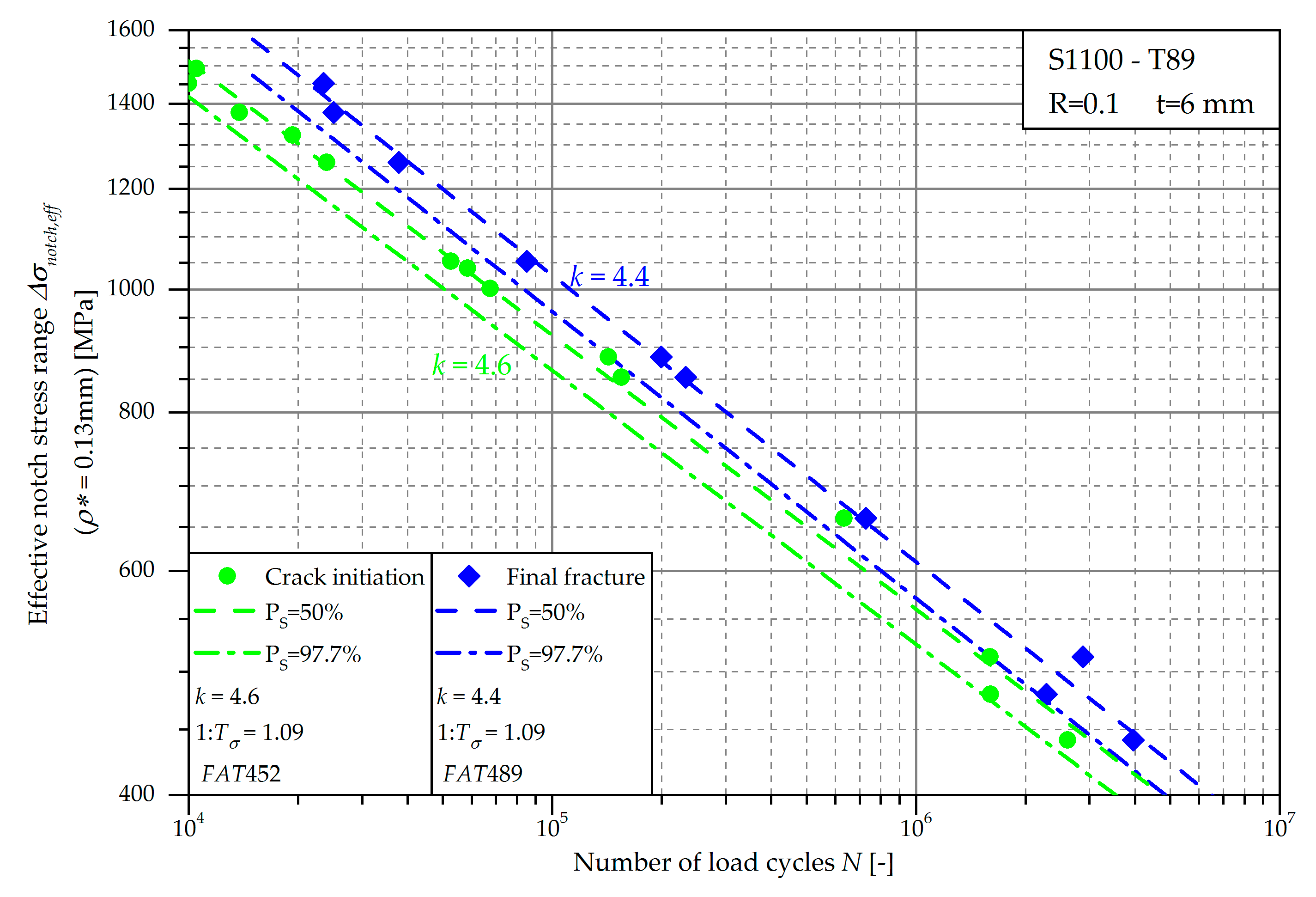
Figure 18 shows the effective notch S-N curve using ρ* = 0.13 mm of specimen failure in blue dye and crack initiation with ath = 0.5 mm in green dye. Table 6 summarizes the effective notch stress fatigue test data. Furthermore, the statistical evaluation including lines of 50% and 97.7% probability of survival are depicted. Some specimens exhibit more than one propagating crack leading to a number of fourteen crack initiation points of ten specimens. In such cases, the effective notch stress values are evaluated at the respective position of the crack initiation points of the particular specimen.
Figure 19 displays the portion of crack initiation life for the ten through cracks with respect to the effective notch stress range. Hereby, the portion of crack propagation life goes along with increasing stress range although large scatter is observed. However, the technical crack initiation phase seems to be the major portion of the fatigue life. In this context, Equation (6) presents a formula for the trace of the crack propagation fraction based on the statistical evaluation of the test results for crack initiation (index init) and burst fracture (index f). The consequential equation is a power law with basis Δσ and the difference of the slopes of the S-N curves as the exponent are applicable for varying the probabilities of survival. However, the scatter indices in the present case are nearly identical causing the equation to be almost independent of the employed probability of survival PS-value. The result of Equation (6) is depicted in Figure 19 for PS = 97.7%.
4.3. Assessment of Crack Propagation Life by Fracture Mechanics
The concluding part of this work deals with the calculation of the stable crack propagation life for all specimens using linear fracture mechanics according to the Paris law. Thereby, each crack initiation point of every specimen is processed using the data presented within this work. Subsequently, the results are compared to the actual fatigue test results.
Two approaches are pursued in this section:
- Start of calculation at the previously determined threshold load cycle number Nth with an initial crack length of ainit = ath = 0.5 mm.
- Calculation from the test start with an initial crack length of ainit = u + 0.1 mm as recommended in [38].
For each of these two approaches three different sets of crack propagation parameters for the Paris law are utilized:
- S1100 base material determined in Section 2.2.;
- IIW parameters for welds suggested in [38]; and
- Best fit parameters resulting by a least square fit of the fatigue test results.
The following three subsections give a comprehensive insight in the applied crack propagation methodology invoking the weight function approach and local geometry-dependent stress distribution approximation formulae.
4.3.1. Crack Propagation Analysis
If the crack initiation phase of a component is significantly exceeded, the fatigue assessment of a structure cannot be continued with stress-based approaches. Thereby, the fatigue action at a crack tip is described by the stress intensity factor (SIF) range ΔK (see Equation (7)). The crack propagation rate for each load cycle is then calculated by crack propagation laws, such as the Paris law (see Equation (4) and [56]).
4.3.2. Weight Functions Approach
The idea behind this technique [68,69,70] is to split a given random stress distribution σ(x) into differential pairs of unit forces opening the crack. The weight function m(x, a) then describes the effect of each differential force on the crack. The stress intensity factor for a given crack length a is, thus, an integration over the crack length (see Equations (8) and (9)). This procedure can be applied for the deepest point ‘a’ and the surface points ‘c’ of a crack by application of the appropriate weight function. In [69], general forms for the weight functions for semi-elliptical surface cracks in plates with finite thickness are published (see Equations (10) and (11)). Figure 20 provides an overview on the crack geometry parameters and the stress distribution at the weld toe due to axial loading.
4.3.3. Stress Distribution
A precise formulation of the local stress distribution in depth σ(x) constitutes an important aspect concerning the proper assessment of the individual stress intensity factors. In [72] an approximation for the stress concentration factor is presented based on the local weld toe radius ρ, the flank angle θ and the sheet thickness t (see Equation (12) and Figure 20). Furthermore, a topology-dependent solution for the stress distribution in depth is shown in [73]. Equation (13) presents the main part of this approximation for pure tension loading. Details for parameter Gm, a correction for the stress distribution away from the stress peak, can be found in the cited work. This set of equations is also referred to and listed in the IIW recommendations [38].
4.3.4. Calculation of Crack Propagation
The methods and approaches presented previously in this section allow an individual calculation of the crack propagation for each point of the specimen under consideration of the local weld toe topography. Thereby, the progress of crack length with load cycle numbers a(N) is calculated by numerical integration of Equation (4) with step size ΔN (see Equation (14)). Within this procedure, the stress intensity factor value ΔK has to be recalculated after each step upon the current crack length value a(N). The value of ΔN is made dependent on the respective number of Nf to ensure at least fifty steps to a final crack length where burst fracture is assumed.
4.3.5. Determination of “Best Fit” Parameters for the Paris Power Law
In addition to the existing material parameters for the S1100 base material and the suggestions according to IIW, an additional set of parameters is determined by best fit to the fatigue test results. This set is characterised by the minimum sum of squared errors, SSE (see Equation (15)). Thereby, the difference of the log values of the calculated and experimental load cycle numbers is used, otherwise high load cycle numbers would be overweighted. The linear elastic crack propagation parameters CP and mP are varied within a meaningful range of and .
4.3.6. Crack Propagation Results
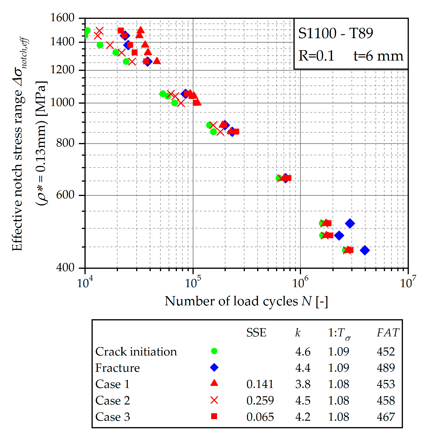
The outcome for cases 1–3, where the crack propagation calculation starts at the determined crack initiation point at a crack length of ainit = 0.5 mm, is illustrated in Figure 21. Case 1 one employs the crack propagation parameters of the S1100 base material. The IIW parameters for welded joints in case 2 deliver a conservative approach across all considered specimens. In general, the use of these parameters leads to a very short crack propagation phase. The application of the S1100 base material parameters in case 1 leads to a non-conservative assessment for specimens with burst fracture below 1 × 10⁵ load cycles. Naturally, the best fit parameters show the best accordance, as expected. Hereby, the exponent mP is similar, but CP is about three times smaller compared to the IIW values. Interestingly, all three parameter sets underestimate the crack propagation phase of the three specimens with the burst fracture above one million load cycles, significantly.
The results of cases 4–6, where the crack initiation phase is neglected, are shown in Figure 22. As already expected based on the previous results, the IIW recommendation in case 5 leads to a very conservative assessment. The use of the S1100 base material parameters in case 4 results in a very steep S-N curve with a slope of just k = 1.7. Here, the specimens exposed to the highest effective notch stress are assessed quite well, but the assessment becomes more and more conservative with the decreasing effective notch stress near to the level of case 5. The best fit parameters reveal once more the best accordance, naturally. However, the assessment is non-conservative for specimens with a burst fracture below 2×10⁵ load cycles.
Table 7 provides an overview on the parameters of the investigated cases. Furthermore, the resulting SSE as well as the result of the statistical evaluation of the consequential S-N curve for each case is shown.
5. Summary and Conclusions
This study deals with the determination of the crack initiation fatigue life and the subsequent macroscopic stable crack propagation life during fatigue tests of ultra high-strength steel S1100 butt joints exhibiting noticeable local undercuts. The underlying experiments show a drop of about 15% in fatigue strength if undercuts are present whereas the inverse slope of about k = 4 remains almost unchanged. Furthermore, a large scattering of the fatigue strength with the size and shape of the undercut is observed. However, the decrease is not as pronounced as one would expect based on the evaluated stress concentration factors using finite element analysis. Here, previous work in [47,51] revealed a Kt of about 1.9–2.5 for regions without undercut compared to values for Kt from 3.5–5.4 for local undercuts.
One main part of this work is the introduction of a simple and cost-effective procedure to determine the crack size during specimen fatigue testing. Therefore, a DSLR-camera is utilized to take pictures of the weld surface in specified intervals. In order to ensure comparable situations for each photo, the fatigue test is interrupted and the upper force is applied to the specimen. An implemented digital image correlation procedure compares each picture with the initial state and calculates the consequential distortion field. Excessive distortions are then identified as crack and monitored until specimen burst rupture. The procedure subsequently provides a load cycle versus surface crack length for each crack within the defined area. The related crack depth is additionally calculated using equations from the literature enabling the determination of a crack initiation load cycle number at a specified crack depth.
Neuber’s stress averaging method is utilized to calculate the effective notch stress range for each specimen. Therefore, the results of FE-analyses for each specimen based on the measured weld geometry are taken. Hereby, values of the microstructural support length of ρ* = 0.1 mm for technical crack initiation and ρ * = 0.13 mm for burst fracture are obtained for minimum scattering regression analysis. These results show good accordance with the published results for similar steel grades.
The second part deals with the application of the presented crack detection procedure on the fatigue tests. It reveals a comparably high portion of crack initiation phase of more than 50% fatigue life even though only specimens with undercuts are evaluated. Basically, the cycles to crack initiation tend to decrease with the increasing effective notch stress range, but quite high scattering is observed.
Finally, a linear elastic crack propagation calculation is performed. The base material featured parameters for the Paris law by SENT-testing. As expected, these show a significant deviation from the suggestions according to IIW for welded joints. However, the evaluated base material S1100 parameters match published results for similar steel types and grades. The crack propagation assessment is started either at the number of cycles to crack initiation, determined with the presented optical detection procedure, or the assessment is carried out from the start of the fatigue test. Furthermore, three different sets of material parameters are used for the case study. The main conclusion of this investigation is that the crack initiation phase is not neglectable. Otherwise, the assessment tends to deliver very conservative results, especially for welds in the high-cycle fatigue domain above one million load cycles. In detail, the material parameters obtained by the IIW recommendation consistently leads to conservative results. If the crack initiation phase is considered, the derived FAT value is just 6 MPa, or 1% higher than the FAT value of the crack initiation S-N curve. Compared to the fracture FAT value, this corresponds to a deviation of −7%. In the case of crack calculation from the start, the result is far more conservative, with a deviation of about −70%. The usage of the base material parameter set delivers non-conservative results for very high effective notch stresses and conservative results for the high-cycle domain. The derived FAT values show similar deviation to the fatigue test result as the evaluations using the IIW-parameters.
Summing up, the provided methodology gives additional insight into the crack initiation and propagation behaviour of high-quality welded butt joints and can act as the basis to compare other steel grades in regard to quality measures, such as undercuts on fatigue testing and crack growth.
Author Contributions
Conceptualization: M.J.O., M.L., M.S. and W.M.; methodology: M.J.O., M.L. and M.S.; software, M.J.O.; validation: M.J.O., M.L. and M.S.; formal analysis: M.J.O.; investigation: M.J.O.; resources: M.L. and W.M.; data curation: M.J.O.; writing—original draft preparation: M.J.O.; writing—review and editing: M.L. and M.S.; visualization: M.J.O.; supervision: M.L. and M.S.; project administration: M.L. and W.M.; funding acquisition: M.L. and W.M.
Funding
Financial support was given by the Austrian Research Promotion Agency (FFG).
Acknowledgments
Special thanks are given to the Austrian Research Promotion Agency (FFG), who founded the research project by funds of the Austrian Ministry for Transport, Innovation and Technology (bmvit) and the Federal Ministry of Science, Research and Economy (bmwfw).
Conflicts of Interest
The authors declare no conflict of interest.
Nomenclature
| Crack depth (mm) | |
| Final crack depth for crack propagation calculation (mm) | |
| ainit | Initial crack depth for crack propagation calculation (mm) |
| Threshold crack depth between crack initiation and propagation (mm) | |
| Crack aspect ratio (–) | |
| Half surface crack length, half width of elliptical crack (mm) | |
| Crack growth rate coefficient according to Paris law (ΔK in MPa√mm; da/dN in mm/cycle) | |
| Young’s modulus (MPa) | |
| Fatigue class according to IIW, stress range Δσ at N = 2·106 load cycles and PS = 97.7% (MPa) | |
| Stress intensity factor (MPa√mm) | |
| Fatigue notch factor (–) | |
| Stress concentration factor (–) | |
| Inverse slope of S/N-curve (–) | |
| Weight function parameters for deepest point of a surface crack | |
| Weight function for deepest point of surface crack | |
| Weight function parameters for surface point of a surface crack | |
| Weight function for surface point of surface crack | |
| mp | Slope of crack growth rate curve according to Paris law (–) |
| Load cycle number (–) | |
| Load cycle number at specimen burst fracture (–) | |
| Load cycle number before start of image acquisition (–) | |
| Interval load cycle number between two image acquisitions (–) | |
| Load cycle number at crack length ath, threshold between crack initiation and propagation (–) | |
| Load cycle number of crack propagation until burst fracture (–) | |
| Transition knee point of S/N-curve (–) | |
| Probability of survival (–) | |
| Load stress ratio (–) | |
| Displacement in y-direction (specimen loading direction) (pixel) | |
| Gradient of displacement in y-direction (–) | |
| Threshold for gradient of displacement in y-direction (–) | |
| Sum of squared errors (–) | |
| Sheet thickness (mm) | |
| Scatter index of S/N-curve, ratio of stress range Δσ at PS = 10% and PS = 90% (–) | |
| Weld toe radius (mm) | |
| Microstructural support length (mm) | |
| Weld flank angle (°) | |
| Stress (MPa) | |
| Recurring indices | |
| Effective value | |
| Nominal value | |
| Notch value | |
| Range, difference of upper and lower value | |
References
- Radaj, D. Review of fatigue strength assessment of nonwelded and welded structures based on local parameters. Int. J. Fatigue 1996, 18, 153–170. [Google Scholar] [CrossRef]
- Lassen, T.; Recho, N. Fatigue Life Analyses of Welded Structures; ISTE: London, UK; Newport Beach, CA, USA, 2006. [Google Scholar]
- Chattopadhyay, A.; Glinka, G.; El-Zein, M.; Qian, J.; Formas, R. Stress analysis and fatigue of welded structures. Weld. World 2011, 55, 2–21. [Google Scholar] [CrossRef]
- Hou, C.-Y.; Charng, J.-J. Models for the estimation of weldment fatigue crack initiation life. Int. J. Fatigue 1997, 19, 537–541. [Google Scholar] [CrossRef]
- Remes, H. Strain-based Approach to Fatigue Strength Assessment of Laser-welded Joints. Ph.D. Thesis, Helsinki University of Technology, Espoo, Finland, 2008. [Google Scholar]
- Lihavainen, V.-M. A Novel Approach for Assessing the Fatigue Strenght of Ultrasonic Impact Treated Welded Structures. Ph.D. Thesis, Lappeenranta University of Technology, Lappeenranta, Finland, 2006. [Google Scholar]
- Peterson, R.E. Notch sensitivity. In Metal Fatigue; Sines, G., Waisman, J.L., Dolan, T.J., Eds.; McGraw-Hill: New York, NY, USA, 1959; pp. 293–306. [Google Scholar]
- Neuber, H. Über die Berücksichtigung der Spannungskonzentration bei Festigkeitsberechnungen. Konstruktion 1968, 20, 245–251. [Google Scholar]
- Radaj, D. Design and Analysis of Fatigue Resistant Welded Structures; Abington: Cambridge, UK, 1990. [Google Scholar]
- Lawrence, F.V.; Ho, N.J.; Mazumdar, P.K. Predicting the fatigue resistance of welds. Ann. Rev. Mater. Sci. 1981, 11, 401–425. [Google Scholar] [CrossRef]
- Seeger, T. Grundlagen für Betriebsfestigkeitsnachweise. Stahlbau-Handbuch, 3rd ed.; Stahlbau-Verl.-Ges: Köln, Germany, 1996; pp. 5–123. [Google Scholar]
- Atzori, B.; Lazzarin, P. Notch sensitivity and defect sensitivity under fatigue loading: Two sides of the same medal. Int. J. Fract. 2001, 107, 1–8. [Google Scholar] [CrossRef]
- Glinka, G. Energy density approach to calculation of inelastic strain-stress near notches and cracks. Eng. Fract. Mech. 1985, 22, 485–508. [Google Scholar] [CrossRef]
- Haibach, E. Betriebsfestigkeit. Verfahren und Daten zur Bauteilberechnung; Springer: Berlin, Germany, 2006. [Google Scholar]
- Krebs, J.; Hübner, P.; Kassner, M. Eigenspannungseinfluss auf Schwingfestigkeit und Bewertung in geschweißten Bauteilen; DVS-Verlag: Düsseldorf, Germany, 2004. [Google Scholar]
- Lieurade, H.-P.; Huther, I.; Maddox, S.J. Recommendations on the Fatigue Testing of Welded Components; LETS Global: Rotterdam, The Netherlands, 2006. [Google Scholar]
- Stoschka, M.; Leitner, M.; Fössl, T.; Posch, G. Effect of high-strength filler metals on fatigue. Weld. World 2012, 56, 20–29. [Google Scholar] [CrossRef]
- Maddox, S.J. The effect of mean stress on fatigue crack propagation a literature review. Int. J. Fract. 1975, 11, 389–408. [Google Scholar]
- Verreman, Y.; Nie, B. Short-crack growth and coalescence along the toe of a manual fillet weld. Fatigue Frac. Eng. Mat. Struct. 1991, 14, 337–349. [Google Scholar] [CrossRef]
- Fricke, W. Fatigue analysis of welded joints: State of development. Mar. Struct. 2003, 16, 185–200. [Google Scholar] [CrossRef]
- Baumgartner, J.; Bruder, T. Influence of weld geometry and residual stresses on the fatigue strength of longitudinal stiffeners. Weld. World 2013, 57, 841–855. [Google Scholar] [CrossRef]
- Leitner, M.; Barsoum, Z.; Schäfers, F. Crack propagation analysis and rehabilitation by HFMI of pre-fatigued welded structures. Weld. World 2016, 60, 581–592. [Google Scholar] [CrossRef] [Green Version]
- Baumgartner, J.; Waterkotte, R. Crack initiation and propagation analysis at welds—Assessing the total fatigue life of complex structures. Mat. Wiss. Werkstofftech. 2015, 46, 123–135. [Google Scholar] [CrossRef]
- Simunek, D.; Leitner, M.; Grün, F. In-situ crack propagation measurement of high-strength steels including overload effects. Proc. Eng. 2018, 213, 335–345. [Google Scholar] [CrossRef]
- Simunek, D.; Leitner, M.; Maierhofer, J.; Gänser, H.-P. Crack growth under constant amplitude loading and overload effects in 1:3 scale specimens. Proc. Struct. Integr. 2017, 4, 27–34. [Google Scholar] [CrossRef]
- Todorov, E.I.; Mohr, W.C.; Lozev, M.G.; Thompson, D.O.; Chimenti, D.E. Detection and Sizing of Fatigue Cracks in Steel Welds with Advanced Eddycurrent techniques. In Proceedings of the AIP Conference—34th Annual Review of Progress in Quantitative Nondestructive Evaluation, Golden, CO, USA, 22–27 July 2007; pp. 1058–1065. [Google Scholar]
- Lamtenzan, D.; Glenn, W.; Lozev, M.G. Detection and Sizing of Cracks in Structural Steel Using the Eddy Current Method; US Department of Transportation Federal Highway Administration FHWA-RD-00-018; Turner-Fairbank Highway Research Center: McLean, VA, USA, 2000.
- Roux, S.; Réthoré, J.; Hild, F. Digital image correlation and fracture: An advanced technique for estimating stress intensity factors of 2D and 3D cracks. J. Phys. D Appl. Phys. 2009, 42, 214004. [Google Scholar] [CrossRef]
- Mathieu, F.; Hild, F.; Roux, S. Identification of a crack propagation law by digital image correlation. Int. J. Fatigue 2012, 36, 146–154. [Google Scholar] [CrossRef] [Green Version]
- Ozelo, R.R.M.; Sollero, P.; Sato, M.; Barros, R.S.V. Monitoring crack propagation using digital image correlation and cod technique. In Proceedings of the COBEM 2009 20th International Congress of Mechanical Engineering, ABCM, Gramado, Brazil, 15–20 November 2009. [Google Scholar]
- Alam, M.M.; Barsoum, Z.; Jonsén, P.; Kaplan, A.F.H.; Häggblad, H.Å. The influence of surface geometry and topography on the fatigue cracking behaviour of laser hybrid welded eccentric fillet joints. Appl. Surf. Sci. 2010, 256, 1936–1945. [Google Scholar] [CrossRef]
- Caccese, V.; Blomquist, P.A.; Berube, K.A.; Webber, S.R.; Orozco, N.J. Effect of weld geometric profile on fatigue life of cruciform welds made by laser/GMAW processes. Mar. Struct. 2006, 19, 1–22. [Google Scholar] [CrossRef]
- Lillemäe, I.; Remes, H.; Liinalampi, S.; Itävuo, A. Influence of weld quality on the fatigue strength of thin normal and high strength steel butt joints. Weld. World 2016, 60, 731–740. [Google Scholar] [CrossRef]
- Rennert, R.; Kullig, E.; Vormwald, M.; Esderts, A.; Siegele, D. Analytical Strength Assessment of Components Made of Steel, Cast Iron and Aluminium Materials in Mechanical Engineering: FKM Guideline, 6th ed.; VDMA-Verl: Frankfurt, Germany, 2012. [Google Scholar]
- Olivier, R.; Köttgen, V.B.; Seeger, T. Welded Joints I—Fatigue Strength Assessment Method for Welded Joints Based on Local Stresses; Forschungshefte No. 143; Forschungskuratorium Maschinenbau: Frankfurt, Germany, 1989. [Google Scholar]
- Olivier, R.; Köttgen, V.B.; Seeger, T. Welded Joints II—Investigation of Inclusion into Codes of a Novel Fatigue Strength Assessment Method for Welded Joints in Steel; No. 180; Forschungskuratorium Maschinenbau: Frankfurt, Germany, 1994. [Google Scholar]
- Morgenstern, C.; Sonsino, C.M.; Hobbacher, A.; Sorbo, F. Fatigue design of aluminium welded joints by the local stress concept with the fictitious notch radius of rf = 1 mm. Int. J. Fatigue 2006, 28, 881–890. [Google Scholar] [CrossRef]
- Hobbacher, A. Recommendations for Fatigue Design of Welded Joints and Components, 2nd ed.; Springer: New York, NY, USA, 2016. [Google Scholar]
- Nykänen, T.; Björk, T.; Laitinen, R. Fatigue strength prediction of ultra high strength steel butt-welded joints. Fatigue Frac. Eng. Mater. Struct. 2013, 36, 469–482. [Google Scholar] [CrossRef]
- Liinalampi, S.; Remes, H.; Lehto, P.; Lillemäe, I.; Romanoff, J.; Porter, D. Fatigue strength analysis of laser-hybrid welds in thin plate considering weld geometry in microscale. Int. J. Fatigue 2016, 87, 143–152. [Google Scholar] [CrossRef]
- Nykänen, T.; Marquis, G.; Björk, T. Effect of weld geometry on the fatigue strength of fillet welded cruciform joints. In Proceedings of the International Symposium on Integrated Design and Manufacturing of Welded Structures; Lappeenranta University of Technology: Lappeenranta, Finland, 2007. [Google Scholar]
- Schork, B.; Kucharczyk, P.; Madia, M.; Zerbst, U.; Hensel, J.; Bernhard, J.; Tchuindjang, D.; Kaffenberger, M.; Oechsner, M.; Zerbst, U. The effect of the local and global weld geometry as well as material defects on crack initiation and fatigue strength. Eng. Fract. Mech. 2018, 198, 103–122. [Google Scholar] [CrossRef]
- Madia, M.; Zerbst, U.; Th. Beier, H.; Schork, B. The IBESS model—Elements, realisation and validation. Eng. Fract. Mech. 2018, 198, 171–208. [Google Scholar] [CrossRef]
- Mashiri, F.R.; Zhao, X.L.; Grundy, P. Effects of weld profile and undercut on fatigue crack propagation life of thin-walled cruciform joint. Thin Walled Struct. 2001, 39, 261–285. [Google Scholar] [CrossRef]
- Steimbreger, C.; Chapetti, M.D. Fatigue strength assessment of butt-welded joints with undercuts. Int. J. Fatigue 2017, 105, 296–304. [Google Scholar] [CrossRef]
- Steimbreger, C.; Chapetti, M.; Hénaff, G. Undercut tolerances in industry from a fracture mechanic perspective. MATEC Web Conf. 2018, 165, 21009. [Google Scholar] [CrossRef]
- Ottersböck, M.J.; Leitner, M.; Stoschka, M.; Maurer, W. Effect of Weld Defects on the Fatigue Strength of Ultra High-strength Steels. Proc. Eng. 2016, 160, 214–222. [Google Scholar] [CrossRef] [Green Version]
- ASTM. Practice for Statistical Analysis of Linear or Linearized Stress-Life (S-N) and Strain-Life (-N) Fatigue Data; E739; ASTM International: West Conshohocken, PA, USA, 2015. [Google Scholar]
- Dengel, D.; Harig, H. Estimation of the fatigue limit by progressively-increasing load tests. Fatigue Frac. Eng. Mat. Struct. 1980, 3, 113–128. [Google Scholar] [CrossRef]
- Sonsino, C.M. Course of SN-curves especially in the high-cycle fatigue regime with regard to component design and safety. Int. J. Fatigue 2007, 29, 2246–2258. [Google Scholar] [CrossRef]
- Ottersböck, M.J.; Leitner, M.; Stoschka, M. Characterisation of actual weld geometry and stress concentration of butt welds exhibiting local undercuts. Eng. Fail. Anal. 2019. in review. [Google Scholar]
- ASTM. Standard Test Method for Measurement of Fatigue Crack Growth Rates; E647; ASTM International: West Conshohocken, PA, USA, 2000. [Google Scholar]
- Tada, H.; Paris, P.C.; Irwin, G.R. The Stress Analysis of Cracks Handbook, 3rd ed.; ASME: New York, NY, USA, 2000. [Google Scholar]
- Beden, S.M.; Abdullah, S.; Ariffin, A.K. Review of fatigue crack propagation models for metallic components. Eur. J. Sci. Res. 2009, 28, 364–397. [Google Scholar]
- Richard, H.A.; Sander, M. Ermüdungsrisse. In Erkennen, Sicher Beurteilen, Vermeiden, 3rd ed.; Springer Vieweg: Wiesbaden, Germany, 2012. [Google Scholar]
- Paris, P.; Erdogan, F. A critical analysis of crack propagation laws. J. Basic Eng. 1963, 85, 528. [Google Scholar] [CrossRef]
- Jones, E.M.C. Improved Digital Image Correlation; Version 4; University of Illinois: Champaign, IL, USA, 2015. [Google Scholar]
- Reu, P.L.; Toussaint, E.; Jones, E.M.C.; Bruck, H.A.; Iadicola, M.; Balcaen, R.; Turner, D.Z.; Siebert, T.; Lava, P.; Simonsen, M. DIC Challenge: Developing images and guidelines for evaluating accuracy and resolution of 2D analyses. Exp. Mech. 2018, 58, 1067–1099. [Google Scholar] [CrossRef]
- Jones, E.M.C. Documentation for Matlab-Based DIC Code; Version 4; University of Illinois: Champaign, IL, USA, 2015. [Google Scholar]
- Ottersböck, M.J. Einfluss von Imperfektionen auf die Schwingfestigkeit hochfester Stahlschweißverbindungen. Ph.D. Thesis, Montanuniversität Leoben, Leoben, Austria, 2019. [Google Scholar]
- Simunek, D.; Leitner, M.; Maierhofer, J.; Gänser, H.-P. Fatigue crack growth under constant and variable amplitude loading at semi-elliptical and V-notched steel specimens. Proc. Eng. 2015, 133, 348–361. [Google Scholar] [CrossRef]
- Engesvik, K.M. Analysis of Uncertainties in the Fatigue Capacity of Welded Joints. Ph.D. Thesis, University of Trondheim, Trondheim, Norway, 1981. [Google Scholar]
- Baumgartner, J. Enhancement of the fatigue strength assessment of welded components by consideration of mean and residual stresses in the crack initiation and propagation phases. Weld. World 2016, 60, 547–558. [Google Scholar] [CrossRef]
- Radaj, D.; Sonsino, C.M.; Fricke, W. Fatigue Assessment of Welded Joints by Local Approaches, 2nd ed.; Woodhead Publishing: Sawston, UK, 2006. [Google Scholar]
- Goyal, R.; Glinka, G. Fracture mechanics-based estimation of fatigue lives of welded joints. Weld. World 2013, 57, 625–634. [Google Scholar] [CrossRef]
- Newman, J.C.; Raju, I.S. Stress-intensity factor equations for cracks in three-dimensional finite bodies, ASTM STP 791. In Fracture Mechanics: Fourteenth Symposium—Volume I: Theory and Analysis; Lewis, J.C., Sines, G., Eds.; ASTM International: West Conshohocken, PA, USA, 1983; pp. I238–I265. [Google Scholar]
- Murakami, Y.; Murakami, Y. Stress Intensity Factors Handbook; Pergamon Press: Oxford, UK, 1990. [Google Scholar]
- Bueckner, H.F. Novel principle for the computation of stress intensity factors. J. Appl. Math. Mech. 1970, 50. [Google Scholar]
- Shen, G.; Glinka, G. Weight functions for a surface semi-elliptical crack in a finite thickness plate. Theor. Appl. Fract. Mech. 1991, 15, 247–255. [Google Scholar] [CrossRef]
- Glinka, G.; Shen, G. Universal features of weight functions for cracks in mode I. Eng. Fract. Mech. 1991, 40, 1135–1146. [Google Scholar] [CrossRef]
- Wang, X.; Lambert, S.B. Stress intensity factors for low aspect ratio semi-elliptical surface cracks in finite-thickness plates subjected to nonuniform stresses. Eng. Fract. Mech. 1995, 51, 517–532. [Google Scholar] [CrossRef]
- Hall, M.S.; Topp, D.A.; Dover, W.D. Parametric Equations for Stress Intensity Factors in Weldments; Project Report TSC/MSH/0244; Technical Software Consultants Ltd.: Milton Keynes, UK, 1990. [Google Scholar]
- Monahan, C.C. Early Fatigue Crack Growth at Welds; Computational Mechanics: Southampton, UK, 1995. [Google Scholar]
Figure 1.
Specimen with weld toe exhibiting a local undercut [47].
Figure 1.
Specimen with weld toe exhibiting a local undercut [47].

Figure 2.
Fatigue test results according to the nominal stress evaluation [47].
Figure 2.
Fatigue test results according to the nominal stress evaluation [47].

Figure 3.
Fracture surface clearly showing the crack initiation point at the undercut (red arrow) [47] (Δσn = 200 MPa, Nf = 2.87×10⁶, R = 0.1).
Figure 3.
Fracture surface clearly showing the crack initiation point at the undercut (red arrow) [47] (Δσn = 200 MPa, Nf = 2.87×10⁶, R = 0.1).

Figure 4.
Stable crack propagation curve of the investigated S1100 base material at R = 0.1.

Figure 5.
Setup for image acquisition: (a) Schematic layout; (b) setup at test rig.

Figure 6.
Schematic block testing programme for image acquisition.

Figure 7.
Reference and last image of an exemplary specimen, Δσn = 400 MPa, Nf = 85,039: (a) Reference image before fatigue test; (b) image at N = 84,000 with crack at upper weld toe; (c) magnification of the crack region of (b).
Figure 7.
Reference and last image of an exemplary specimen, Δσn = 400 MPa, Nf = 85,039: (a) Reference image before fatigue test; (b) image at N = 84,000 with crack at upper weld toe; (c) magnification of the crack region of (b).

Figure 8.
Result of image correlation at N = 84,000: (a) Displacement field sy in vertical (y)-direction; (b) vertical gradient of vertical displacement field s’y.
Figure 8.
Result of image correlation at N = 84,000: (a) Displacement field sy in vertical (y)-direction; (b) vertical gradient of vertical displacement field s’y.

Figure 9.
Binarized matrix of Figure 8 indicating crack regions.
Figure 9.
Binarized matrix of Figure 8 indicating crack regions.

Figure 10.
Gradient field s’y of Figure 8 with marked results of the crack identification process.
Figure 10.
Gradient field s’y of Figure 8 with marked results of the crack identification process.

Figure 11.
Surface crack length 2c over load cycle number N.

Figure 12.
Position and extension of determined cracks marked at specimen surface and comparison of the crack identification procedures result with the final fracture surface: (a) N = 60,000; (b) N = 84,000; (c) fracture surface at Nf = 85,039 with three clearly visible crack initiation points.
Figure 12.
Position and extension of determined cracks marked at specimen surface and comparison of the crack identification procedures result with the final fracture surface: (a) N = 60,000; (b) N = 84,000; (c) fracture surface at Nf = 85,039 with three clearly visible crack initiation points.

Figure 13.
Comparison of beach marks length and assessed crack length: (a) Fracture surface with the surface length measurement of visible bench marks; (b) development of the crack length over the load cycle number.
Figure 13.
Comparison of beach marks length and assessed crack length: (a) Fracture surface with the surface length measurement of visible bench marks; (b) development of the crack length over the load cycle number.


Figure 14.
Fracture surfaces used for validation of the calculated crack length: (a) Specimen 1; Δσn = 400 MPa, Nf = 85,039; (b) specimen 2; Δσn = 600 MPa, Nf = 30,871.
Figure 14.
Fracture surfaces used for validation of the calculated crack length: (a) Specimen 1; Δσn = 400 MPa, Nf = 85,039; (b) specimen 2; Δσn = 600 MPa, Nf = 30,871.

Figure 15.
Measurement of not-through crack size by fitting a semi-ellipse: (a) Specimen 1; (b) specimen 2.
Figure 15.
Measurement of not-through crack size by fitting a semi-ellipse: (a) Specimen 1; (b) specimen 2.

Figure 16.
S-N curves for specimen fracture depending upon the microstructural support length ρ*.

Figure 17.
Development of slope, scatter index and FAT value with microstructural support length; (a) Crack initiation; (b) burst fracture.
Figure 17.
Development of slope, scatter index and FAT value with microstructural support length; (a) Crack initiation; (b) burst fracture.

Figure 18.
S-N curve including crack initiation life and cycles to final rupture of all investigated specimens.
Figure 18.
S-N curve including crack initiation life and cycles to final rupture of all investigated specimens.

Figure 19.
The fraction of the crack initiation life in total fatigue life over the effective notch stress range.
Figure 19.
The fraction of the crack initiation life in total fatigue life over the effective notch stress range.

Figure 20.
Sketch of the weld geometry including weld and crack geometry parameters.

Figure 21.
S-N curve of crack propagation calculation starting at crack initiation.

Figure 22.
S-N curve of crack propagation calculation from the start.


Table 1.
Mechanical properties of the base and filler material.
| Material | Yield Strength σy (MPa) | Tensile Strength σu (MPa) | Elongation A (%) | Impact Work ISO-V KV (J) |
|---|---|---|---|---|
| Base, S1100 | ≥1100 | ≥1140 | ≥8 | ≥ 27 @ −20 °C |
| Filler, T89 | ≥890 | ≥940 | ≥15 | ≥ 47 @ −40 °C |
Table 2.
Definition of intervals for image acquisition.
| Current Load Cycle Number N (–) | Interval between Image Acquisition Ninterval (–) | ||
|---|---|---|---|
| 0≤ | N | <100,000 | 2000 |
| 100,000≤ | N | <400,000 | 5000 |
| 400,000≤ | N | <800,000 | 10,000 |
| 800,000≤ | N | <1500,000 | 25,000 |
| 1500,000 ≤ | N | 50,000 | |
Table 3.
Comparison between the measured and assessed surface crack length.
| Beach Mark | Measured Crack Length 2c (mm) | Assessed Crack Length 2c (mm) | Deviation (%) | |
|---|---|---|---|---|
| No. | N (–) | |||
| 1 | 740,000 | 17.94 | 18.23 | 1,62 |
| 2 | 700,000 | 11.98 | 11.97 | −0,08 |
| 3 | 660,000 | 9.52 | 9.52 | 0 |
| 4 | 620,000 | 8.00 | 7.92 | −1.00 |
| 5 | 580,000 | 6.84 | 6.72 | −1.75 |
| 6 | 540,000 | 6.00 | 6.00 | 0 |
Table 4.
Crack propagation of selected not-through cracks and comparison to fracture surface measurement.
Table 4.
Crack propagation of selected not-through cracks and comparison to fracture surface measurement.
| Specimen 1 | Specimen 2 | ||||
|---|---|---|---|---|---|
| Number of Load Cycles N (–) | Assessed Crack Length 2c (mm) | Measured Crack Length 2c after Final Rupture (mm) | Number of Load Cycles N (–) | Assessed Crack Length 2c (mm) | Measured Crack Length 2c after Final Rupture (mm) |
| 60,000 | 1.41 | 7.76 | 20,000 | - | 3.70 |
| 62,000 | 2.31 | 22,000 | - | ||
| 64,000 | 2.56 | 24,000 | 1.19 | ||
| 66,000 | 2.70 | 26,000 | 1.70 | ||
| 68,000 | 2.95 | 28,000 | 2.39 | ||
| 70,000 | 3.34 | 30,000 | 3.24 | ||
| 72,000 | 3.59 | 30,871 | 3.67 * | ||
| 74,000 | 3.98 | ||||
| 76,000 | 4.24 | ||||
| 78,000 | 4.49 | ||||
| 80,000 | 5.01 | ||||
| 82,000 | 5.65 | ||||
| 84,000 | 6.93 | ||||
| 85,039 | 7.66 * | ||||
* Quadratic extrapolation.
Table 5.
Statistical evaluation for crack initiation and total fatigue life.
| Evaluation Method | Crack Initiation | Burst Fracture | ||||
|---|---|---|---|---|---|---|
| Slope k (–) | FAT Value (MPa) | Scatter Index 1:Tσ (–) | Slope k (–) | FAT Value (MPa) | Scatter Index 1:Tσ (–) | |
| Nominal stress | 4.43 | 160 | 1.30 | 4.20 | 176 | 1.29 |
| Eff. notch stress (ρ* = 0.4 mm) | 4.68 | 307 | 1.16 | 4.46 | 337 | 1.15 |
| Eff. notch stress (ρ* = 0.3 mm) | 4.68 | 340 | 1.14 | 4.45 | 372 | 1.13 |
| Eff. notch stress (ρ* = 0.2 mm) | 4.66 | 392 | 1.11 | 4.44 | 427 | 1.10 |
| Eff. notch stress (ρ* = 0.13 mm) | 4.64 | 452 | 1.09 | 4.43 | 489 | 1.09 |
| Eff. notch stress (ρ* = 0.1 mm) | 4.62 | 489 | 1.08 | 4.43 | 523 | 1.10 |
| Notch stress (Kt) | 4.37 | 626 | 1.41 | 4.38 | 650 | 1.51 |
Table 6.
Overview on local stress concentration and fatigue test data for each crack initiation point.
Table 6.
Overview on local stress concentration and fatigue test data for each crack initiation point.
| Specimen No. | Kt (–) | Kf (–) | Δσeff (MPa) | Nth (–) | Nf (–) | Nth /Nf (%) | |
|---|---|---|---|---|---|---|---|
| ρ = 0.10 mm | ρ = 0.13 mm | ||||||
| 1 | 3.93 | 2.60 | 2.42 | 1453.5 | 10,000 | 23,497 | 43 |
| 4.50 | 2.69 | 2.49 | 1492.2 | 10,520 | - | - | |
| 2 | 3.37 | 2.36 | 2.21 | 884.5 | 142,840 | 199,292 | 71 |
| 3 | 3.97 | 2.60 | 2.40 | 479.8 | 1601,800 | 2281,981 | 70 |
| 4 | 5.61 | 2.89 | 2.63 | 1052.6 | 52,650 | 85,039 | 53 |
| 4.75 | 2.83 | 2.60 | 1039.5 | 58,530 | - | - | |
| 4.45 | 2.71 | 2.50 | 1001.2 | 67,580 | - | - | |
| 5 | 5.82 | 2.80 | 2.57 | 513.6 | 1596,300 | 2873,617 | 52 |
| 6 | 3.50 | 2.33 | 2.20 | 660.0 | 635,190 | 728,340 | 87 |
| 7 | 3.92 | 2.36 | 2.21 | 441.5 | 2610,560 | 3958,013 | 67 |
| 8 | 3.33 | 2.24 | 2.10 | 1259.4 | 24,000 | 37,839 | 66 |
| 4.60 | 2.40 | 2.20 | 1322.7 | 19,330 | - | - | |
| 9 | 3.81 | 2.49 | 2.30 | 1378.7 | 13,790 | 25,060 | 52 |
| 10 | 4.61 | 3.06 | 2.84 | 852.9 | 155,070 | 232,717 | 67 |
Table 7.
Summary of the investigated crack propagation cases including the statistical evaluation of the consequential S-N curves.
Table 7.
Summary of the investigated crack propagation cases including the statistical evaluation of the consequential S-N curves.
| Start Crack Length ainit (mm) | Start Load Cycle Number Nstart (–) | Parameters for Paris Law | SSE (–) | Statistical Evaluation of S-N Curve | |||||
|---|---|---|---|---|---|---|---|---|---|
| Material | CP | mP | Slope k (–) | FAT Value (MPa) | Scatter Index 1:Tσ (–) | ||||
| Case 1 | 0.5 | Nth | S1100 | 8.35×10⁻¹⁰ | 1.72 | 0.141 | 3.80 | 453 | 1.077 |
| Case 2 | 0.5 | Nth | IIW | 5.21×10⁻¹³ | 3.00 | 0.259 | 4.47 | 458 | 1.076 |
| Case 3 | 0.5 | Nth | Best fit | 1.78×10⁻¹³ | 2.90 | 0.065 | 4.17 | 467 | 1.084 |
| Case 4 | u + 0.1 | 0 | S1100 | 8.35×10⁻¹⁰ | 1.72 | 6.710 | 1.73 | 92 | 1.239 |
| Case 5 | u + 0.1 | 0 | IIW | 5.21×10⁻¹³ | 3.00 | 14.251 | 3.03 | 147 | 1.243 |
| Case 6 | u + 0.1 | 0 | Best fit | 1.00×10⁻¹³ | 2.85 | 0.985 | 2.92 | 339 | 1.255 |
© 2019 by the authors. Licensee MDPI, Basel, Switzerland. This article is an open access article distributed under the terms and conditions of the Creative Commons Attribution (CC BY) license (http://creativecommons.org/licenses/by/4.0/).
Share and Cite
MDPI and ACS Style
Ottersböck, M.J.; Leitner, M.; Stoschka, M.; Maurer, W. Crack Initiation and Propagation Fatigue Life of Ultra High-Strength Steel Butt Joints. Appl. Sci. 2019, 9, 4590. https://doi.org/10.3390/app9214590
AMA Style
Ottersböck MJ, Leitner M, Stoschka M, Maurer W. Crack Initiation and Propagation Fatigue Life of Ultra High-Strength Steel Butt Joints. Applied Sciences. 2019; 9(21):4590. https://doi.org/10.3390/app9214590
Chicago/Turabian StyleOttersböck, Markus J., Martin Leitner, Michael Stoschka, and Wilhelm Maurer. 2019. "Crack Initiation and Propagation Fatigue Life of Ultra High-Strength Steel Butt Joints" Applied Sciences 9, no. 21: 4590. https://doi.org/10.3390/app9214590
Note that from the first issue of 2016, this journal uses article numbers instead of page numbers. See further details here.