Tone Mapping of High Dynamic Range Images Combining Co-Occurrence Histogram and Visual Salience Detection

Abstract

One of the significant qualities of the human vision, which differentiates it from computer vision, is so called attentional control, which is the innate ability of our human eyes to select what visual stimuli to pay attention to at any moment in time. In this sense, the visual salience detection model, which is designed to simulate how the human visual system (HVS) perceives objects and scenes, is widely used for performing multiple vision tasks. This model is also in high demand in the tone mapping technology of high dynamic range images (HDRIs). Another distinct quality of the HVS is that our eyes blink and adjust brightness when objects are in their sight. Likewise, HDR imaging is a technology applied to a camera that takes pictures of an object several times by repeatedly opening and closing a camera iris, which is referred to as multiple exposures. In this way, the computer vision is able to control brightness and depict a range of light intensities. HDRIs are the product of HDR imaging. This article proposes a novel tone mapping method using CCH-based saliency-aware weighting and edge-aware weighting methods to efficiently detect image salience information in the given HDRIs. The two weighting methods combine with a guided filter to generate a modified guided image filter (MGIF). The function of the MGIF is to split an image into the base layer and the detail layer which are the two elements of an image: illumination and reflection, respectively. The base layer is used to obtain global tone mapping and compress the dynamic range of HDRI while preserving the sharp edges of an object in the HDRI. This has a remarkable effect of reducing halos in the resulting HDRIs. The proposed approach in this article also has several distinct advantages of discriminative operation, tolerance to image size variation, and minimized parameter tuning. According to the experimental results, the proposed method has made progress compared to its existing counterparts when it comes to subjective and quantitative qualities, and color reproduction.

1. Introduction

A camera is designed to perform an HVS-like task—to capture the surroundings and provide information for higher-level processing. Given this similarity, a naïve conception would be that a physical scene captured by a camera and viewed on a display device should invoke the exact same response as observing the scene directly. However, this is very seldom the case, for a number of reasons. First of all, there are insufficient depth cues in the captured image, and there are differences in color and brightness between the captured image and what the HVS perceives. The camera and the HVS also have different dynamic ranges. Therefore, the camera and the display devices are unable to cover wider ranges of luminance which the HVS can detect simultaneously, and this implies that there is more visual information available in the real-life scene than what can be captured and reproduced. For instance, when a camera captures an object in a dark indoor environment in front of a bright window, one has to choose between properly exposed background and foreground, while the other information is lost in dark or saturated image areas, respectively. However, it is usually not a problem for the human eyes to simultaneously register both foreground and background. Hence, the limitation of the camera compared to the human eyes becomes evident.

HDR imaging is able to get information in both dark and bright image regions and it matches or outperforms the HVS in its capability to capture the dynamic range. Therefore, to enjoy images that exploit the full potential of HVS, equally good quality cameras and display devices are needed. Fortunately, today, HDR scenes can be efficiently captured by using high-end cameras, new sensor technologies or computational photography methods that can extract HDRIs from several differently exposed low dynamic range images (LDRIs). Yet display technology is lagging behind and a majority of display today has moderate contrast rates and is unable to faithfully reproduce HDR content. To overcome such limitations, tone mapping methods are used to efficiently scale contrast of HDRIs and to reproduce color on standard LDR display devices, without significant loss of important features and detailed information. That is, tone mapping operators (TMOs) are used to compress the dynamic range of HDRIs and thereby fill the gap between the current HDR imaging technique and the limitation of visualizing HDRIs on conventional LDR display devices. TMOs provide an alternative method of HDR display technology. Although HDR display technology is rapidly advancing, there still remains a strong need to realize HDRIs on LDR display devices [1].

Over the past several decades, a lot of research and study were carried out in tone mapping such as enhancement of contrast, brightness, and visibility of LDRI [2,3,4]. Reinhard and his colleagues [5] proposed a photographic practice-based method using the automatic dodging-and-burning technology. Their method provided a practical approach to compressing the dynamic range, but a circular surround restricts the scope of performance, likely causing halos. Fairchild and Johnson [6] applied an Image Color Appearance Model (iCAM) to chromatics, converting the RGB color space into CIE XYZ tristimulus values. However, the conversion caused saturation loss and the resultant darker resulting image. Kuang and his colleagues [7] designed an iCAM-based algorithm called iCAM06. The algorithm split HDRI into the base layer and the detail layer, using the piece-wise bilateral filter. However, it had a drawback that the resulting image had color saturation reduction. Kim et al. [8] came up with a new approach to correcting saturation loss and saturation reduction alike, using the inverse compensation in a bid to improve iCAM06. Mantiuk et al. [9] proposed a color correction operator which scales the tone, as well as preserves original image colors. Reinhard and his colleagues [10] proposed a color rendering operator to address computational complexity of the above-mentioned approaches. So, the computational cost sharply decreased, but the resulting image still appeared darker. Choi and his colleagues [11] published a color rendering operator which uses global tone mapping to compress dynamic range. The method made good progress in cutting color or hue shift and color leakage compared to previous methods. However, a well-known problem occurred in that the detailed information was lost in the given HDR image, caused by the global TMO. Recently, P. Cyriac et al. [12] proposed a method to convert HDR images into LDR image using histogram clipping approach and gamma correction. Still, the detailed information was lost in the given HDR image. H. Hristova [13] proposed various guided image editing methods. The resulting images were smoothed and contaminated with noises. Another method proposed by H.-H. Choi et al. [14] employed a function of cone response. Global tone mapping method suggested by Y. Kinoshita et al. [15] uses a single parameter.

In this regard, this paper proposes a novel approach to tone mapping of HDRIs, which has two parts: the chromatics-based TMO and the chromatic adaptive transform (CAT). An image histogram (IH), used in this new approach, is a representation of the pixel value distribution based on the given HDRIs and has several strengths such as image without noise, tolerance to image rotation, size variation, and more. The CCH using an IH has long been published as a technology to compress image and video, conduct visual search and recognize objects by selecting necessary features from the given image. In addition, the CCH-based visual saliency detection is used to estimate the attentional gaze of observers viewing a scene, which is faster and easier to implement and involves minimal parameter tuning. Therefore, the TMO in the proposed method adopts CCH-based saliency aware weighting and edge aware weighting methods. The two methods combined with a guided image filter to create a MGIF which thereby decomposes an image into a base layer and a detail layer. The base layer is used to acquire global tone mapping, which contributes to compressing the dynamic range, as well as preserving sharp edges in the given HDRIs. The proposed TMO is a combination of two parameters [16,17]: key value of scene and visual gamma. Key value of scene is intended to scale the contrast (or brightness) of the given HDRI whereas visual gamma is designed to compress the dynamic range based on the contrast sensitivity function (CSF) [18]. In this way, they contribute to reducing the luminance shift and hue shift (or color shift), as well as controlling the dynamic range according to the given HDRIs. As a result, the parameters, key value of scene and visual gamma, are automatically set.

After the performance of TMO, the CAT is used to cope with mismatch between real-world scenes and displayed images. Instead of using the fixed luminance value (F = 1 for average, F = 0.8 for dim and dark) per se from the iCAM06 [7], the CAT in the proposed method modifies the luminance factor to avoid color leakage and color shift (or hue shift). The proposed method mainly contributes to reducing halos and avoiding loss of detailed information without color or hue shift and color leakage in the given HDRIs.

2. Proposed Method

As discussed in the introduction section, the conventional local and global tone mapping techniques have several drawbacks such as halos and loss of detailed information after correcting the color. Such problems, however, can be overcome by adopting the CCH which extracts salient regions from a given image. The proposed tone mapping method has two parts: the proposed TMO and the modified CAT. The proposed TMO uses the CCH-based salience detection model where Lu’s method [19] and a guided filter [20] are combined to create a MGIF. The MGIF then can extract the salient regions and separate a base layer and a detail layer in an image. The base layer is processed through the proposed TMO to compress the dynamic range and improve the contrast of the given HDRIs. Then, the CAT is employed to cope with dynamic range differences between real-world scenes and displayed images.

2.1. Construction of Image Co-Occurrrence Histogram

A histogram of an image (IH) is the distribution of the pixel values in the given image. It has several distinct advantages of image without noise, tolerance to image rotation, size variation, and more. A traditional, one-dimensional IH presents occurrence of each image value only, but completely discards information about how image pixels are distributed in a certain location despite its high importance to the perception of an image. Noticeably, a two-dimensional image co-occurrence histogram (ICH) can indicate both occurrence and co-occurrence of image pixels and be used as a means of calculating the salient region.

From this fact, let $I_h\left(x, y\right)=\left[X_h\left(x, y\right),Y_h\left(x, y\right),Z_h\left(x, y\right)\right]$ be a pixel in an HDRI. In the proposed method, the ICH is used to modify the salience detection model that is similar to the saliency modeling in [19] in order to process an HDRI. An ICH of one of the CIE XYZ color components, $X_h$, in the intensity domain, $H_X$, is defined as

$$H_X=\left[h_X\left(m, n\right)\right], 1\le m, n\le L,$$

(1)

where $H_X$ is a symmetric square matrix of $L\times L$, representing occurrence and co-occurrence of a pixel value. The element $h_X\left(m, n\right)$ indicates the frequency of occurrence of a pixel value at the condition of intensities m and n in the local neighborhood window of $w\times w$ ($w=3$). In other words, an ICH, $H_X$, counts how many times a pixel value with intensities m and n occurs. Likewise, the ICH can depict a global distribution of intensities as well.

Figure 1 shows the product of plotting an ICH. (a) is an original ‘tulip’ image, and (b) shows an ICH of a gray-scale tulip image. Most pixel pairs are concentrated along the diagonal of the ICH, and the peak is located at the center of the pixel value in the histogram below. The result is similar to what is suggested in [21].

Next, the global and local distributions of intensities are used in detecting image saliency. In general, the principle of contrast states that rare or infrequent visual features in a global image context give rise to high saliency values. From this viewpoint and motivated by the Boltzmann’s entropy theorem [22], a logarithm relationship is applied to Equation (1) as

$$P_{log}=p_{log}\left(m, n\right)=-\ln \left(p\left(m, n\right)\right)$$

(2)

where $p\left(m, n\right)$ refers to a probability mass function (PMF), which is the product of normalizing the ICH matrix $H_X$. However, saliency is not correlated with occurrence and co-occurrence, so an inverted PMF ${\overline{P}}_v$ is calculated as

$${\overline{P}}_v=\left[\overline{p}\left(m, n\right)\right]=\{\begin{array}{cc}0, & if p_{log}\left(m, n\right)=0\\ 0,& if p_{log}\left(m, n\right)>\frac{1}{U_X}\\ \frac{1}{U_X}- p_{log}\left(m, n\right)& if p_{log}\left(m, n\right)\le \frac{1}{U_X}\end{array}$$

(3)

In Equation (3), ${\overline{P}}_v$ is set for 0 in the absence of intensity pairs within the given image and if $P_{log}$ is larger than a threshold, $\frac{1}{U_X}$. Meanwhile, $U_X$ refers to the frequency of occurrence whose value is not zero in $H_X$.

Next, saliency is computed by ${\overline{P}}_v$. For each pixel at a location $\left(x, y\right)$, image saliency, $S_v\left(x, y\right),$ is calculated as

$$S_v\left(x, y\right)={\displaystyle \sum }_{x^{\prime }=x-z}^{x+z}{\displaystyle \sum }_{y^{\prime }=y-z}^{y+z}\overline{p}\left(i\left(x, y\right), i\left(x^{\prime }, y^{\prime }\right)\right),$$

(4)

where $z$ represents the size of a neighborhood window. The notations $i\left(x, y\right)$ and $i\left(x^{\prime }, y^{\prime }\right)$ define image values at locations $\left(x, y\right)$ and $\left(x^{\prime }, y^{\prime }\right)$, respectively, and $\overline{p}\left(i\left(x, y\right), i\left(x^{\prime }, y^{\prime }\right)\right)$ is therefore the element of ${\overline{P}}_v$ indexed by $i\left(x, y\right)$ and $i\left(x^{\prime }, y^{\prime }\right)$.

Image brightness and color aside, the ICH can also plot the image gradient orientation which is often closely correlated with the perceptual visual saliency. If the gradient is unsigned, the histogram channels spread in the range of 0 to 180 degrees, whereas if signed, the histogram channels spread in the range of 0 to 360 degrees. As the edge direction alone is considered in calculating the image gradient orientation, the scope of image gradient orientation is 180 bins, ranging from 1 to 180. A gradient orientation ICH, $H_o$, of 180 × 180 bins is plotted like the $H_X$ in Equation (1). The inverted PMF function ${\overline{P}}_o$ and the saliency $S_o\left(x, y\right)$ can be similarly constructed as specified in Equations (2)–(4), respectively.

The saliency information is extracted by computing a combination of the intensity domain and the gradient orientation domain as

$$S=S_{va}+S_{oa}$$

(5)

where

$$S_{va}\left(x, y\right)=\frac{1}{9}{\displaystyle \sum }_{m=-1}^1{\displaystyle \sum }_{n=-1}^1{S}_v\left(x+m, y+n\right),$$

(6)

$$S_{oa}\left(x, y\right)=\frac{1}{9}{\displaystyle \sum }_{m=-1}^1{\displaystyle \sum }_{n=-1}^1{S}_o\left(x+m, y+n\right),$$

(7)

where $S_v$ refers to the saliency of intensity and $S_o$ is the saliency of the gradient orientation.

Based on Equation (5), the saliency is further used to calculate a saliency-aware weighting (SAW) (${\mathsf{\Gamma }}_b\left(x,y\right))$ for an HDRI. To calculate an edge-aware weighting (EAW) (${\mathsf{\Gamma }}_e\left(x, y\right)$), the local variance and mean of the given HDRI are used. The final weighting function,$W\left(x, y\right)$, is described as

$$W\left(x, y\right)=\frac{{\mathsf{\Gamma }}_e\left(x,y\right)}{{\mathsf{\Gamma }}_b\left(x,y\right)}$$

(8)

here

$${\mathsf{\Gamma }}_b\left(x, y\right)=\{\begin{array}{cc}1, & if S_F\left(x, y\right)\le 1\\ S_F\left(x, y\right),& otherwise\end{array}$$

(9)

and

$$S_F\left(x, y\right)=\frac{S\left(x, y\right)}{\frac{1}{N}{{\displaystyle \sum }}_{x=1}^N{{\displaystyle \sum }}_{y=1}^{N}S\left(x, y\right)}$$

(10)

where $S\left(x, y\right)$ refers to the resulting value of Equation (5) and $N$ is the total number of pixels in the given image. In the process of detecting image saliency, a pixel $\left(x, y\right)$ with a larger ${\mathsf{\Gamma }}_b\left(x, y\right)$ takes priority over the others. If a pixel $(x, y$) belongs to an attention-salient region, the value of ${\mathsf{\Gamma }}_b\left(x, y\right)$ is 1 and above. Therefore, a higher priority is given to a pixel in an attention-salient region. This is similar to the ability of attentional control of our HVS. Our human eyes are more likely to pay attention to information in the attention-salient region than elsewhere.

Furthermore, a luminance value, which is defined as one of the CIE XYZ color components, $Y$, is used in calculating an EAW [23] in Equation (8). The luminance value in the log domain is expressed as $L_h\left(x, y\right)$. Let ${\sigma }_{L_h, {\rho }_2}\left(x, y\right)$ and ${\mu }_{L_h, {\rho }_2}\left(x, y\right)$ be the standard deviation and the average value of the component $L_h$ in ${\mathsf{\Omega }}_{{\rho }_2}\left(x, y\right)$. If $L_h\left(x, y\right)$ is located at the edge and $L_h\left(x^{\prime },y^{\prime }\right)$ is in the flat area, ${\sigma }_{L_{h, {\rho }_2}}^2\left(x, y\right)/{\mu }_{L_{h, {\rho }_2}}^2\left(x, y\right)$ is larger than ${\sigma }_{L_{h, {\rho }_2}}^2\left(x^{\prime }, y^{\prime }\right)/{\mu }_{L_{h, {\rho }_2}}^2\left(x^{\prime }, y^{\prime }\right)$, which implies a higher weighting in Equation (9). From this observation, ${\mathsf{\Gamma }}_e\left(x, y\right)$ is calculated by using normalized local standard deviations of all the pixels as

$${\mathsf{\Gamma }}_e\left(x, y\right)=\frac{1}{N\times N}{\displaystyle \sum }_{x^{\prime }=1}^N{\displaystyle \sum }_{y^{\prime }=1}^N\frac{{\left(\frac{{\sigma }_{L_{h, {\rho }_2}}^2\left(x, y\right)+{\nu }_1}{{\mu }_{L_{h, {\rho }_2}}^2\left(x, y\right)+{\nu }_2}\right)}^{\varsigma }}{{\left(\frac{{\sigma }_{L_{h, {\rho }_2}}^2\left(x^{\prime }, y^{\prime }\right)+{\nu }_1}{{\mu }_{L_{h, {\rho }_2}}^2\left(x^{\prime }, y^{\prime }\right)+{\nu }_2}\right)}^{\varsigma }}$$

(11)

where $\varsigma$ is a constant value, ${\nu }_1$ is added in order to avoid instability which can occur if ${\sigma }_{L_{h, {\rho }_2}}^2\left(x, y\right)$ is zero. The ${\nu }_1$ is calculated as ${\left(0.001\ast L\right)}^2$, with L, the dynamic range of the given image [24]. ${\nu }_2$ is a small constant that is intended to prevent dividing by 0.

The ${\mathsf{\Gamma }}_e\left(x, y\right)$ is larger than 1 if the $\left(x, y\right)$ is placed at the edge while it is less than 1 if the $\left(x, y\right)$ is in a smooth area. A larger weighting tends to be assigned to a pixel at the edge rather than in a flat area according to the proposed weighting ${\mathsf{\Gamma }}_e\left(x, y\right)$ in Equation (11).

2.2. Estimation of Detail Layer

Psychophysical studies reveal that the HVS tends to select attention-salient regions before handling the process of reducing the complexity of the scene in their sight, while HVS is still aware of the information outside the attention-salient regions [25]. That is the motivation of developing the visual salience detection model.

The luminance component of an HDRI is split as

$$Y_h\left(x, y\right)=Y_{base}\left(x, y\right)Y_{detail}\left(x, y\right)$$

(12)

where $Y_{base}\left(x, y\right)$ and $Y_{detail}\left(x, y\right)$ refer to the base layer and the detail layer, respectively, obtained by using the MGIF. The detail layer $Y_{detail}\left(x, y\right)$ has a narrow dynamic range. In contrast, the base layer $Y_{base}\left(x, y\right)$ could have more varying dynamic ranges. As proven by the “just noticeable difference (JND)” experiment [26], the transformation performed by the retina of the HVS can be approximately realized by applying the log function. Motivated by this finding, an image is applied to a log function and decomposed as

$$L_h\left(x, y\right)=\log \left(Y_h\left(x, y\right)\right)=L_{base}\left(x, y\right)+L_{detail}\left(x, y\right)$$

(13)

where $L_{base}\left(x, y\right)$ and $L_{detail}\left(x, y\right)$ are $log\left(Y_{base}\left(x, y\right)\right)$ and $log\left(Y_{detail}\left(x, y\right)\right)$, respectively.

Like the guided filter in ref. [20], $L_{base}\left(x, y\right)$ is assumed to have a following relationship with the $L_h\left(x, y\right)$ in the window ${\mathsf{\Omega }}_{{\rho }_2}\left(x^{\prime },y^{\prime }\right)$, described as

$$L_{base}\left(x, y\right)= a_{x^{\prime }, y^{\prime }}{L}_h\left(x, y\right)+b_{x^{\prime }, y^{\prime }}, \forall \left(x, y\right)\in {\mathsf{\Omega }}_{{\rho }_2}\left(x^{\prime },y^{\prime }\right)$$

(14)

where $a_{x^{\prime }, y^{\prime }}$ and $b_{x^{\prime },y^{\prime }}$ are supposed to be constant in the window ${\mathsf{\Omega }}_{{\rho }_2}\left(x^{\prime },y^{\prime }\right)$. The coefficients ($a_{x^{\prime }, y^{\prime }}$,$b_{x^{\prime },y^{\prime }}$) are obtained by minimizing the difference between $L_h\left(x, y\right)$ and $L_{base}\left(x, y\right)$ while maintaining the relation model, Equation (14). Clearly, the smoothness of Equation (14) depends on the value of $a_{x^{\prime }, y^{\prime }}$. Hence, $a_{x^{\prime }, y^{\prime }}$ and $b_{x^{\prime }, y^{\prime }}$ are calculated as

$$a_{x^{\prime }, y^{\prime }}=\frac{W\left(x^{\prime },y^{\prime }\right){\sigma }_{L_{h, {\rho }_2}}^2\left(x^{\prime },y^{\prime }\right)}{W\left(x^{\prime },y^{\prime }\right){\mu }_{L_{h, {\rho }_2}}^2\left(x^{\prime },y^{\prime }\right)+\lambda }$$

(15)

$$b_{x^{\prime }, y^{\prime }}=\left(1-a_{x^{\prime }, y^{\prime }}\right){\mu }_{L_{h, {\rho }_2}}\left(x^{\prime },y^{\prime }\right)$$

(16)

A pixel value of $L_{base}\left(x, y\right)$ is involved in all pixels in the overlapping window ${\mathsf{\Omega }}_{{\rho }_2}\left(x,y\right)$, and $L_{base}\left(x, y\right)$ is described as

$$L_{base}\left(x, y\right)={\overline{a}}_{x, y}{L}_h\left(x, y\right)+{\overline{b}}_{x, y}$$

(17)

where

$${\overline{a}}_{x,y}=\frac{1}{\left|{\mathsf{\Omega }}_{{\rho }_2}\left(x, y\right)\right|}{\displaystyle \sum }_{x^{\prime },y^{\prime }\in {\mathsf{\Omega }}_{{\rho }_2}\left(x, y\right)}{a}_{x^{\prime }, y^{\prime }},$$

(18)

$${\overline{b}}_{x,y}=\frac{1}{\left|{\mathsf{\Omega }}_{{\rho }_2}\left(x, y\right)\right|}{\displaystyle \sum }_{x^{\prime },y^{\prime }\in {\mathsf{\Omega }}_{{\rho }_2}\left(x, y\right)}{b}_{x^{\prime }, y^{\prime }},$$

(19)

For instance, Figure 2 shows that both the attentional gaze and the detail layer are extracted by using Equation (17) based on the observer’s attentional gaze. (a) is a collection of several original HDRIs. (b) is a collection of the resulting images by Equation (17). The attentional gaze is efficiently extracted as shown in the resulting images. Furthermore, the resulting images are also efficiently smoothed. (c) is a collection of the resulting images of extracting the detail layer. The detailed information in the given HDRIs is accurately extracted as shown in the resulting images. Therefore, if these resulting images are applied to perform the TMO, the resulting images of TMO will deliver better performance and also preserve the detailed information in the given HDRIs. This is one of the main goals of the proposed method as well as one of the key differences between Choi’s method [11] and the proposed TMO.

2.3. Tone Mapping Operator (TMO)

The previous sub-section has introduced how to extract the salient regions. Now this sub-section will discuss the proposed TMO in detail. The proposed TMO is given the images in CIE XYZ tristimulus values, likely linear and absolute values. The absolute luminance Y channel is in the unit of cd/m². The input luminance value $L_{in, i}$ is the product of combining the key value of the scene and the visual gamma value, as

$$L_{in, i}\left(x, y\right)={\alpha }_i{L}_i{\left(x, y\right)}^{{\gamma }_{v, i}};i\in \left\{X, Y, Z\right\}$$

(20)

where $L_i$ is the luminance value and ${\alpha }_i$ refers to the key value of the scene, which is used to enhance the contrast (or brightness) in the given HDRI as suggested in ref. [16]. The parameter ${\gamma }_{v, i}$ is defined as a visual gamma [17]. Now the conventional tone mapping methods commonly use the gamma correction to scale the dynamic range, but they show several color distortion problems. To overcome such significant drawbacks, the proposed method adopts the visual gamma as a means to control the dynamic range according to the input HDRIs, with the key value of scene and visual gamma correction set automatically as a result. Figure 3 shows the characteristic curve resulting from using the visual gamma correction based on [17]. Therefore, the visual gamma correction will bring better performance in scaling dynamic range than conventional gamma correction methods.

Based on Equation (20), the proposed TMO ($L_{TMO, i}$) is described as

$$L_{TMO, i}\left(x, y\right)=\frac{L_i\left(x, y\right)}{1-L_{in, i}\left(x, y\right)};i\in \left\{X, Y,Z\right\}$$

(21)

where $L_i\left(x, y\right);i\in \left\{X, Y, Z\right\}$ is the CIE XYZ tristimulus values in the given HDRIs. $L_{TMO}$ is the final outcome of the tone-mapping.

2.4. Chromatic Adaptation Transform (CAT) Based on CMCCAT2000

Chromatic adaptation is defined as the HVS’ ability to adjust to changes in illumination in order to preserve the appearance of object colors. It allows us to perceive object colors stably and constantly even under different illuminations. However, digital imaging technology is far behind the HVS in chromatic adaptation. For example, a digital camera is unable to adapt to changes in illumination colors wholly and partially. In order to perform chromatic adaptation like the HVS, the computer vision has to take the changes in illumination colors into account and transform the tristimulus values of its captured image. Such transformations are called chromatic adaptation transforms (CATs). For this reason, the resulting image undergoes the CAT based on CMCCAT2000 [27]. The CMCCAT2000-based CAT operation is able to predict the mechanism of the HVS using all available data sets, which is more accurate than other versions. Using the tone-mapped image resulting from Equation (21), the transformation to estimate the chromatic adaptation is calculated as

$$\begin{gathered} \left(\begin{array}{c}R\\ G\\ B\end{array}\right)=M\left(\begin{array}{c}X\\ Y\\ Z\end{array}\right), \left(\begin{array}{c}{R}_w\\ G_w\\ B_w\end{array}\right)=M\left(\begin{array}{c}{X}_w\\ Y_w\\ Z_w\end{array}\right), \left(\begin{array}{c}{R}_{wr}\\ G_{wr}\\ B_{wr}\end{array}\right)=M\left(\begin{array}{c}{X}_{wr}\\ Y_{wr}\\ Z_{wr}\end{array}\right) , \\ M=\left(\begin{array}{ccc}0.7982& 0.3389& -0.1371\\ -0.5918& 1.5512& 0.0406\\ 0.0008& 0.0239& 0.9753\end{array}\right), \end{gathered}$$

(22)

where $R_w$, $B_w$, $G_w$ and $X_w$, $Y_w$, $Z_w$ refer to R, G, B and X, Y, Z each for the white point. $X_{wr}$, $Y_{wr}$, and $Z_{wr}$ refer to the reference white in reference illumination.

The D, which includes incomplete adaptation to be used in CMCCAT2000, is optimized to give the least color difference, and the last term in Equation (23) is included to consider dark luminance effects. The D value is given by the luminance value of test and reference adapting field ($\mathrm{cd}/{\mathrm{m}}^2$), $L_{A1}$ and $L_{A2}$, and the surround luminance factor F, as

$$D=F\left\{0.08 lo{g}_{10}\left[0.5\left(L_{A1}+L_{A2}\right)\right]+0.76-0.45\left(L_{A1}-L_{A2}\right)/\left(L_{A1}+L_{A2}\right)\right\},$$

(23)

where

$$F=0.2k^4\left(5L_A\right)+0.1\left(1-k^4\right){\left(5L_A\right)}^{\frac{1}{3}},$$

(24)

$$L_A=L_w/5,$$

(25)

$$k=\frac{1}{5L_A},$$

(26)

where $L_{A1}$ and $L_{A2}$ are the luminance values ($\mathrm{cd}/{\mathrm{m}}^2$) of the reference adapting field, respectively. Both are the product of dividing the illuminance value in lux by π and multiplying it by $Y_b/100$. Here, $Y_b$ is any luminance factor other than the object’s luminance. Most color appearance models (CAMs) assume that the observer has a single state of visual adaptation, but the important visual adaptation for appearance matching images is in fact affected by the surround conditions as well as luminous images. The effect of luminous images becomes more highlighted in dim or dark surroundings. Unfortunately, the method, CMCCAM2000, improves the issue of saturation or colorfulness but produces some unexpected artifacts, such as color or hue shift and color leakage. Hence, Equation (24) is used in the CAT instead of surround luminance (F = 1 for average surround, or F = 0.8 for dim- and dark-surround) to deal with a problem such as color shift and leakage, and a wide variety of conditions in a real scene. In Equation (23), if D is above 1 or below 0, it has to be set to 1 or 0. $L_A$ is a function of adaptation luminance, and accounts for 20% of the adaptation white ($L_w$). $R_c$, $B_c$, and $G_c$ values are the chromatically adapted cone responses obtained from the following equations, especially with the D cone response applied

$$R_c=R\left[\alpha \left(R_{wr}/R_w\right)+1-D\right],$$

(27)

$$G_c=G\left[\alpha \left(G_{wr}/G_w\right)+1-D\right],$$

(28)

$$B_c=B\left[\alpha \left(B_{wr}/B_w\right)+1-D\right],$$

(29)

where

$$\alpha =\frac{D{Y}_w}{Y_{wr}},$$

(30)

where $R_w$, $B_w$, $G_w$ and $X_w$, $Y_w$, $Z_w$ values represent corresponding R, G, B and X, Y, Z values for the white point, respectively. $X_{wr}$, $Y_{wr}$, and $Z_{wr}$ values refer to the reference white in reference illumination.

From Equation (27) through Equation (29), the corresponding tristimulus value, $X_c$, $Y_c$, and $Z_c$ are calculated as

$$\begin{gathered} \left(\begin{array}{c}{X}_c\\ Y_c\\ Z_c\end{array}\right)=M^{-1}\left(\begin{array}{c}{R}_c\\ G_c\\ B_c\end{array}\right), \\ {M}^{-1}=\left(\begin{array}{ccc}1.076450& -0.237662& 0.161212\\ 0.410964& 0.554342& 0.034694\\ -0.010954& -0.013389& 1.024343\end{array}\right), \end{gathered}$$

(31)

The forward mode converts the tristimulus values of an example under a non-daylight illumination (say, A) into those of the corresponding colors under a daylight illumination, typically D65. In estimating corresponding colors from a daylight to a non-daylight illumination, the reverse mode should be used, and the reverse mode of CMCCAT2000 is described as

$$\left(\begin{array}{c}{R}_w\\ G_w\\ B_w\end{array}\right)=M\left(\begin{array}{c}{X}_w\\ Y_w\\ Z_w\end{array}\right), \left(\begin{array}{c}{R}_{wr}\\ G_{wr}\\ B_{wr}\end{array}\right)=M\left(\begin{array}{c}{X}_{wr}\\ Y_{wr}\\ Z_{wr}\end{array}\right) , \left(\begin{array}{c}{R}^{\prime }\\ G^{\prime }\\ B^{\prime }\end{array}\right)=M\left(\begin{array}{c}{X}_c\\ Y_c\\ Z_c\end{array}\right),$$

(32)

$$D=F\left\{0.08 lo{g}_{10}\left[0.5\left(L_{A1}+L_{A2}\right)\right]+0.76-0.45\left(L_{A1}-L_{A2}\right)/\left(L_{A1}+L_{A2}\right)\right\},$$

(33)

where

$$F=0.2k^4\left(5L_A\right)+0.1\left(1-k^4\right){\left(5L_A\right)}^{\frac{1}{3}}$$

(34)

where $L_{A1}$ and $L_{A2}$ values are the luminance of reference adapting field. $L_A$ is a function of adaptation luminance and accounts for 20% of the adaptation white ($L_w$). D represents the incomplete adaptation.

From Equation (32), the transformed chromatic adaptation values, $R^{\prime }$, $G^{\prime }$, and $B^{\prime }$ are obtained as

$$R^{″}=R^{\prime }\left[\alpha \left(R_{wr}/R_w\right)+1-D\right],$$

(35)

$$G^{″}=G^{\prime }\left[\alpha \left(G_{wr}/G_w\right)+1-D\right],$$

(36)

$$B^{″}=B^{\prime }\left[\alpha \left(B_{wr}/B_w\right)+1-D\right],$$

(37)

where

$$\alpha =\frac{D{Y}_w}{Y_{wr}},$$

(38)

where $R_w$,$G_w$, $B_w$ and $X_w$, $Y_w$, $Z_w$ values represent corresponding R, G, B and X, Y, Z values for the white point, respectively. $X_{wr}$, $Y_{wr}$, and $Z_{wr}$ values refer to the reference white in reference illumination.

From Equations (37)–(39), the resulting image is finally obtained by achieving an inversion process as

$$\left(\begin{array}{c}X\\ Y\\ Z\end{array}\right)=M^{-1}\left(\begin{array}{c}{R}^{″}\\ G^{″}\\ B^{″}\end{array}\right),$$

(39)

If any of the values $R^{″}$, $G^{″}$, and $B^{″}$ are negative, then their positive equivalent must be used.

3. Experimental Results and Evaluations

This section presents comparative evaluations of the proposed method and three conventional methods: iCAM06 [7], Reinhard’s method [10], and Choi’s method [11]. The experiments apply several publicly available HDRIs widely used in assessing tone mapping performance and the images captured under five standard illuminations (D, SWF, TL84, A, and UV). The several widely used HDRIs and the captured images under five illuminants are tone-mapped by the proposed method and the three conventional methods respectively and their resulting images are compared with each other.

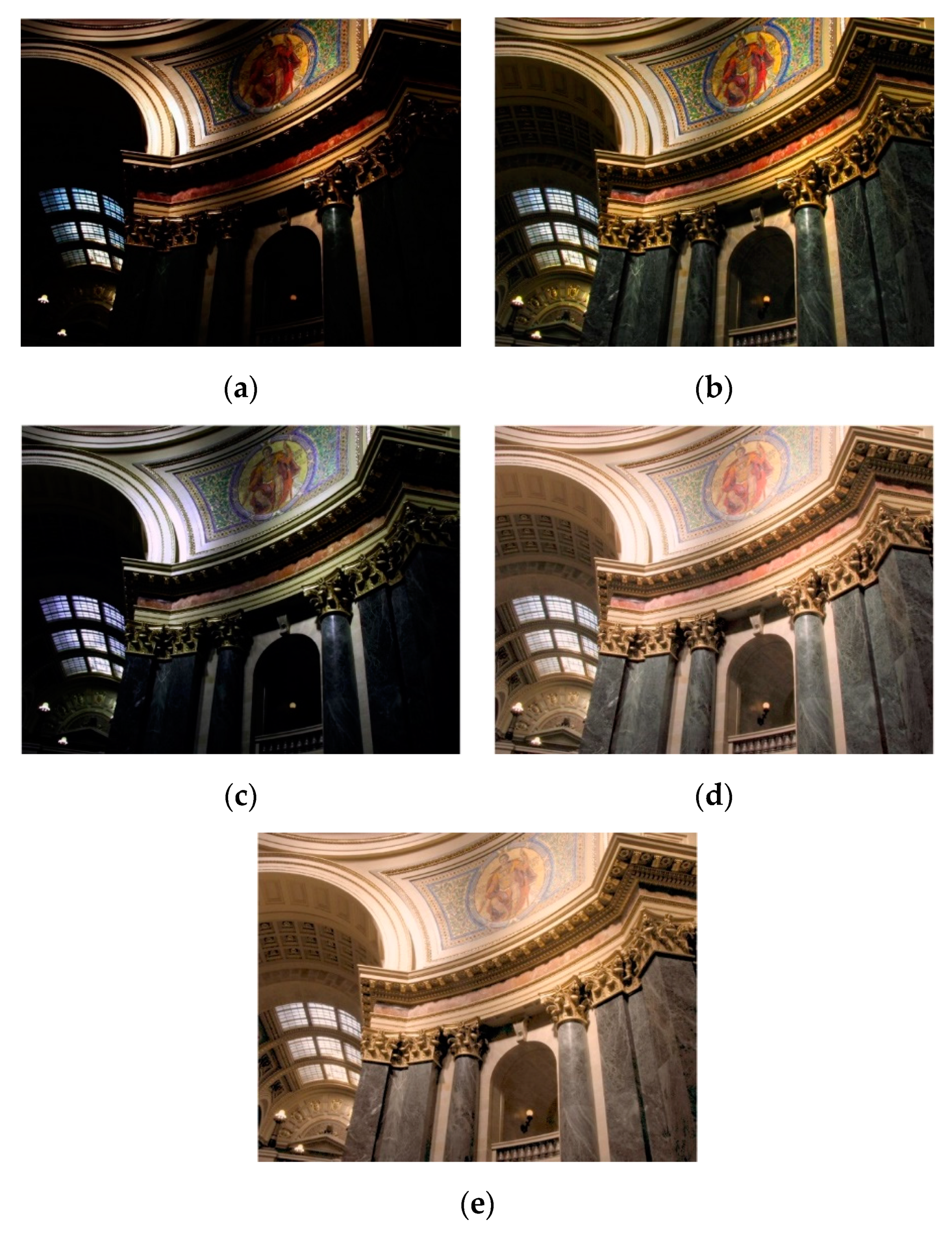
Figure 4, Figure 5 and Figure 6 are the original HDRIs and their resulting images processed by tone mapping techniques of iCAM06 [7], Reinhard’s method [10], Choi’s method [11], and the proposed method. For each Figure, (a) shows an original HDRI and (b) shows its resulting image processed by the iCAM06 tone mapping method where its MATLAB codes are implemented and parameters are fixed as suggested in [7]. The contrast in the resulting image tone-mapped by iCAM06 has improved relative to that of its original image. However, the contrast is still low with the resulting image overall much darker. The reason is that the luminance factor is a model of adaptation to the changing illumination levels and the luminance adaptation has a sigmoidal relation used to compress the dynamic range. Therefore, as color shift in a given chromaticity moves the sigmodal curve to the left, the luminance factor likely decreases. Furthermore, iCAM06, one of color appearance models, produces several unwanted artifacts such as color or hue shift and color leakage due to the surround factor. (c) is the resulting image tone-mapped by Reinhard’s method [10] which is implementation of the MATLAB codes according to [10]. By taking the 90th percentile in a given luminance max value, Reinhard’s method computes and chooses the maximum scene luminance such that the small but extremely bright region does not bias further computation. Hence, the contrast in the original image can no longer increase especially in the low contrast region of image. The resulting image makes some progress in terms of color leakage and color or hue shift problems, but it is still overall as dark as that of iCAM06. This is why the loss of detailed information takes place in the entire resulting image. (d) shows the resulting image processed by Choi’s method [11]. Choi’s method is designed to overcome the limitations of the iCAM06 and Reinhard’s methods such as color leakage, color or hue shift, and an overall darker resulting image. Yet this method, which is based on the global tone mapping to reduce time cost, causes loss of detailed information in the overall resulting image after color correction. To address this problem and represent detailed information in the tone-mapped resulting image, an ICH-based tone mapping method is proposed, which has the strengths of image without noise, tolerance to image rotation, size variation, and more as described in the introduction section. (e) is the resulting image processed by the proposed method. The resulting image overall represents more detailed information and also its contrast markedly increases without color distortion such as color leakage and color or hue shift compared to those from the conventional methods, especially iCAM06 and Reinhard’s method. As supporting evidence, other images are processed and compared in Figure 7.

Table 1. Comparative evaluation of computational cost between iCAM06, Reinhard’s method, Choi’s method, and the proposed method (units: per seconds).

	iCAM06	Reinhard’s Method	Choi’s Method	Proposed Method
Computational cost	8.6238	1.986	5.89	29.7170

is a summary of comparative evaluation results of computational cost between iCAM06, Reinhard’s method, Choi’s method and the proposed method. The used computer consists of Intel (R) Core (TM) i7-6700 CPU @ 3.40GHz 3.41 GHz and 16.0GB RAM. The proposed method has a higher computational cost. It is noticeable that there is trade-off between computational cost and performance.

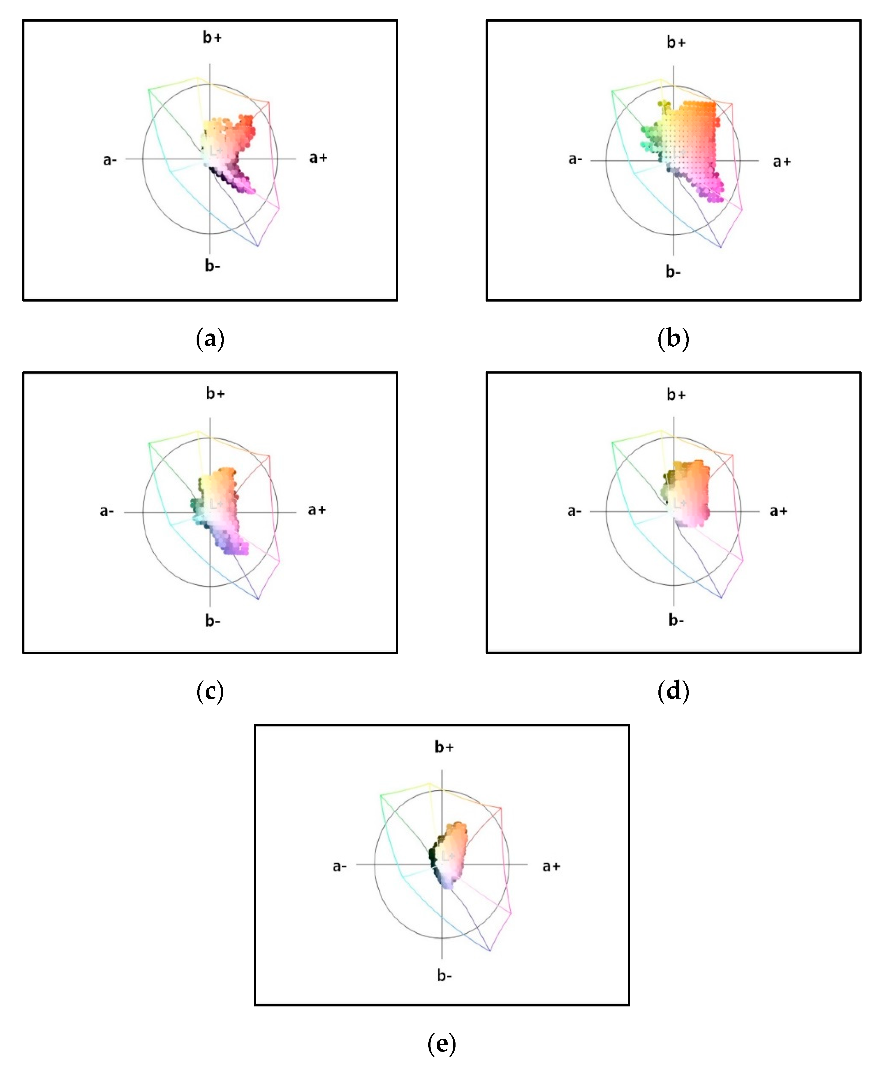
To evaluate color or hue shift and color leakage in perspective, in Figure 8, CIE LAB color space-based gamut area [28] is used to measure the target image (Figure 4). (a) shows the gamut area of an original image and the L* axis is from top to bottom (L+ for top and L- for bottom). The maximum L+ is 100 and indicates a perfect reflecting diffuser. The minimum L- is zero and appears black. The a* and b* axes have no limits. Positive a* (or a+) is red and negative a* (or a-) is green. Positive b* (or b+) appears yellow and negative b* (or b-) appears blue. The gamut area of the original image is biased in both red and red-blue directions. (b) shows the gamut area of the resulting image tone-mapped by the iCAM06. The biased regions increase in both red and red-blue directions. Noticeably, the resulting image is overall affected by color or hue shift and color leakage. (c) shows the gamut area of the resulting image processed by Reinhard’s method. The gamut area is biased in a blue direction. In contrast, (d) shows that the biased region decreases in the gamut area in the resulting image tone-mapped by Choi’s method. (e) shows the gamut area in the resulting image tone-mapped by the proposed method where the biased region decreases to some extent, compared to those of its conventional counterparts. Figure 9 is the histograms of the images in Figure 4 and represents the dynamic range in the L* color space. The brightness of the resulting image processed by the proposed method increases compared to those of its conventional counterparts. Figure 10 shows the resulting tone-mapped images of the captured images under five standard illuminations. Figure 11 is CIEL*a*b* [29], Ref [30]—based comparative evaluation of color difference ($\mathsf{\Delta }{E}_{ab}$) between the original images and the resulting tone-mapped images as shown in Figure 10. As compared in Figure 11, the proposed method results in lower differences than its conventional counterparts, meaning the proposed method records the state-of-the-art performance in terms of color reproduction.

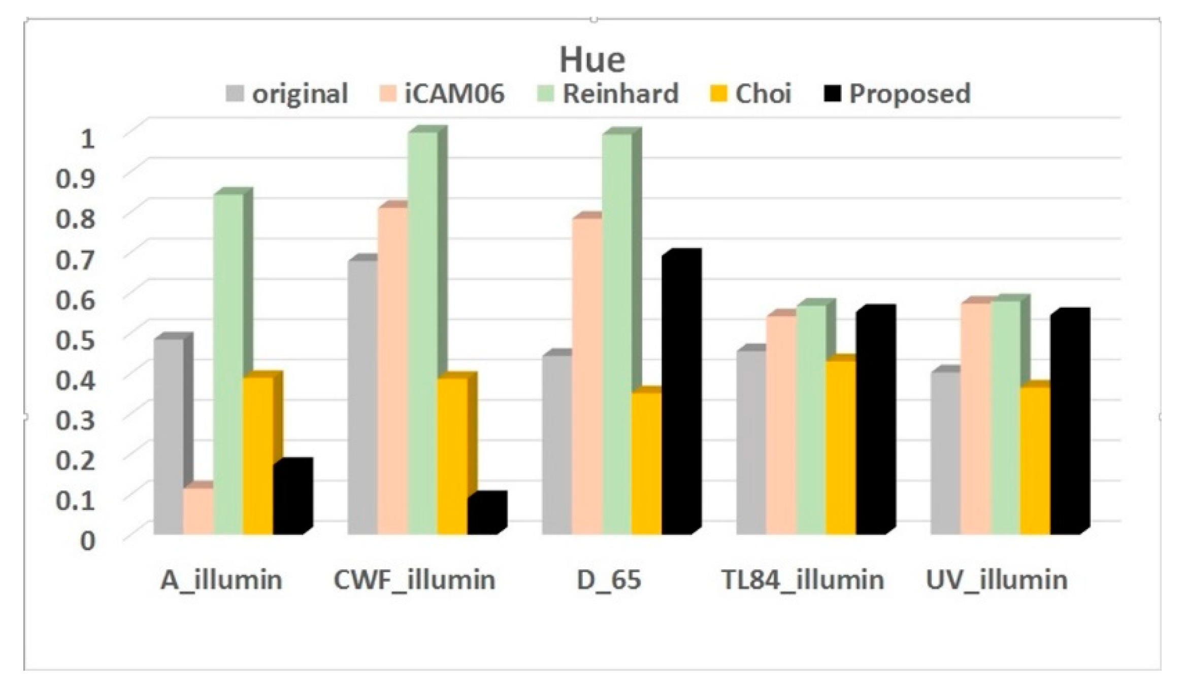
Next, CIEL*a*b*-based colorfulness [29] is assessed and compared in Figure 12. The proposed method records higher values than its conventional counterparts except CWF and D65 which in fact perform better in Reinhard’s method than the proposed method. Furthermore, CIEL*a*b*-based Hue [30] is evaluated and compared in Figure 13. In the Hue comparative evaluation, the proposed method records lower scores than its conventional counterparts in several images like A and CWF, and in the other images Choi’s method alone records lower scores. The result also shows that images like A and CWF tone-mapped by conventional methods, especially iCAM06 and Reinhard’s methods, introduce a larger hue shift relative to the proposed method.

As a subjective evaluation, a psychophysical experiment was conducted. The color vision test was joined by a total of 15 male participants and used 30 different images captured under 5 standard illuminations and then processed by various tone mapping methods. In the test, the 30 images went through color rendering process and the outcomes were assessed and compared in the categories of the color reproduction, brightness, and colorfulness. These test images were displayed on 32” LG 32QK500C which has been calibrated. The resolution of the monitor is 2560 × 1440 (QHD) at 30–83 kHz. Its brightness is max = 300 cd/m² and min = 250 cd/m². Therefore, the contrast ratio is approximately 1000:1, DFC: Mega. The viewing distance for the test is 80 cm. The screen is behind a dark mask. The maximum time allowed to choose between two tone-mapped images is 13 s which was decided based on a pilot study. All 15 observers are aged between 30 and 34. They are working for M.D. and Ph.D. in the color image rendering field in a university and therefore have a deep understanding of their task. For the psychophysical experiment, a pair of images were compared. The 30 images were processed by the iCAM06, Reinhard’s method, Choi’s method, and the proposed method and the resulting images were compared. The experiment was conducted in a dark environment to overcome a veiling glare limit in a white or bright background. The parameters used in each algorithm are fixed at the values suggested in the paper of each method mentioned above. The observers judged a pair of images at a time and gave “1” to the image they judged accepted and “0” to the image they judged rejected. When they judged the image a draw, they gave “0.5” to each image. The scores were all added and converted into the preference scores [31]. Figure 14 shows the product of the psychophysical experiment. The higher preference scores were given to the proposed method relative to its conventional counterparts.

4. Conclusions

The goal of tone mapping is scaling the dynamic ranges of original HDRIs as well as reproducing and preserving color in resulting tone-mapped images. A tone mapping method proposed in this article consists of the CCH-based TMO and CMCCAT2000-based CAT. The CCH-based TMO is a combination of the key value of the scene and the visual gamma and it enables the resulting, tone-mapped HDRIs to preserve and represent the detailed information. The purpose of the key value of the scene is to adjust contrast while the visual gamma is intended to control the dynamic range as well as avoid luminance shift and hue shift (color shift). The CAT processes the resulting tone-mapped images, thereby addressing the mismatch between the real-life scene and the displayed image and contributing to making the displayed image closer to the real-life scene.

In the experimental results, the proposed method demonstrates better representation of the detailed information in the resulting images as well as reduced color shift, luminance shift, and color leakage, compared to the conventional methods. In the CIELab color space-based measurement and comparison of color difference, the proposed method results in lower color differences than its conventional counterparts, which supports that the proposed method has improved in the color reproduction. In the colorfulness assessment and comparison conducted with the given, original HDRIs, the proposed method records higher values than its conventional counterparts except for a few images such as CWF and D65. In the hue measurement and comparison, the proposed method has larger hue values than the other methods. As a subjective evaluation, the psychophysical experiment is performed on 30 different images captured under five different standard illuminations and tone-mapped by several conventional methods and the proposed method in this article. As a result, the proposed method resulted in higher preference scores than its conventional counterparts. The proposed method proves to perform better than its conventional counterparts in several evaluations such as color difference formula, psychophysical experiment, and the like. We will continue to study and solve remaining problems in the timeline of the near future.

References

- Reinhard, E.; Heidrich, W.; Debevec, P.; Pattanaik, S.; Ward, G.; Myszkwski, K. High Dynamic Range Imaging: Acquisition, Display, and Image-Based Lighting; Morgan Kaufmann: San Mateo, CA, USA, 2010. [Google Scholar]
- Yeganch, H.; Wang, Z. High Dynamic Range Image Tone Mapping by Maximizing a Structural Fidelity Measure; ICASSP: Vancouver, ON, Canada, 2013; pp. 1879–1883. [Google Scholar]
- Yeganch, H.; Wang, Z. Objective quality assessment of tone-mapped images. IEEE Trans. Image Process 2013, 22, 657–667. [Google Scholar] [CrossRef] [PubMed]
- Nawaria, M.; Da Silba, P.; Le Callet, P.; Pepion, R. Tone mapping based HDR compression: Does it affect visual experience? Signal Process. Image Commun. 2014, 29, 257–276. [Google Scholar] [CrossRef]
- Reinhard, E.; Stark, M.; Shirley, P.; Ferwerda, J. Photographic Tone Reproduction for Digital Images. ACM Trans. Graph. 2002, 21, 267–276. [Google Scholar] [CrossRef]
- Fairchild, M.D.; Johnson, G.M. iCAM framework for image appearance, differences and quality. J. Electron. Imaging 2004, 13, 126–138. [Google Scholar] [CrossRef]
- Kuang, J.; Johnson, G.M.; Fairchild, M.D. iCAM06: A refined image appearance model for HDR image rendering. J. Vis. Commun. Image Represent 2007, 18, 406–414. [Google Scholar] [CrossRef]
- Hwi-Gang, K.; Sung-Hark, L.; Tae-Wuk, B.; Kyu-Ik, S. Color saturation compensation in iCAM06 for high-chroma HDR image. IEICE Trans. Fundam. Electron. Commun. Comput. Sci. 2011, 94, 2353–2357. [Google Scholar]
- Mantiuk, R.; Tomaszewska, A.; Heidrich, W. Color correction for tone mapping. Comput. Graph. Forum 2009, 28, 193–202. [Google Scholar] [CrossRef]
- Reinhard, E.; Pouli, T.; Kunkel, T.; Long, B.; Ballestad, A.; Damberg, G. Calibrated Image Appearance Reproduction. ACM Trans. Graph. 2012, 31, 201. [Google Scholar] [CrossRef]
- Choi, H.H.; Kim, G.-S.; Yun, B.-J. Modeling a color-rendering operator for high dynamic range images using a cone-response function. J. Electron. Imaging 2015, 24, 053005. [Google Scholar] [CrossRef] [Green Version]
- Cyriac, P.; Kane, D.; Bertalmio, M. Optimized Tone Curve for In-Camera Image Processing. In Proceedings of the IS&T Electronic imaging Conference, San Francisco, CA, USA, 14–18 February 2016. [Google Scholar]
- Hristova, H. Example-Guided Image Editing. Ph.D. Thesis, University of Rennes, Rennes, France, 2017. [Google Scholar]
- Choi, H.-H.; Kim, E.-S.; Yun, B.-J. Tone Mapping High Dynamic Range image using Cone Response Function based on CAM16. In Proceedings of the 2019 Eleventh International Conference on Ubiquitous and Future Network (ICUFN), Zagreb, Croatia, 2–5 July 2019; pp. 639–641. [Google Scholar]
- Kinoshita, Y.; Shiota, S.; Kiya, H. Reinhard’s global operator based inverse Tone mapping with one parameter. In Proceedings of the 2017 Eighth International Workshop on Signal Design and Its Applications in Communications (IWSDA), Sapporo, Japan, 24–28 September 2017; pp. 49–53. [Google Scholar]
- Akyuz, A.O.; Reinhard, E. Color appearance in high-dynamic-range imaging. J. Electron. Imaging 2006, 15, 033001. [Google Scholar]
- Lee, S.-H.; Jang, S.-W.; Kim, E.-S.; Sohng, K.-I. The Quantitative Model for Optimal Threshold and Gamma of Display Using Brightness Function. IEICE 2006, 89, 1720–1723. [Google Scholar] [CrossRef]
- Lee, G.-Y.; Lee, S.-H.; Kwon, H.-J.; Sohng, K.I. Visual sensitivity correlated tone reproduction for low dynamic range images in the compression field. Opt. Eng. 2014, 53, 113111. [Google Scholar] [CrossRef] [Green Version]
- Lu, S.; Tan, C.; Lim, J. Robust and Efficient Saliency Modeling from Image Co-Occurrence Histogram. IEEE Trans. Pattern Anal. Mach. Intell. 2014, 36, 195–201. [Google Scholar] [PubMed]
- He, K.; Sun, J.; Tang, X. Guided Image Filtering. IEEE Trans. Pattern Anal. Mach. Intell. 2013, 35, 1397–1409. [Google Scholar] [CrossRef] [PubMed]
- Zhang, L.; Li, A. Region-of-Interest Extraction Based on Saliency Analysis of Co-Occurrence Histogram in High Spatial Resolution Remote Sensing Images. IEEE J. Sel. Top. Appl. Earth Obs. Sens. 2015, 8, 2111–2124. [Google Scholar] [CrossRef]
- Goldstein, S.; Lebowitz, J.L. On the (Boltzmann) entropy of non-equilibrium system. Phys. D Nonlinear Phenom. 2004, 193, 53–66. [Google Scholar] [CrossRef]
- Li, Z.; Zheng, J.; Zhu, Z.; Yao, W.; Wu, S. Weighted Guided Image Filtering. IEEE Trans. Image Process. 2015, 24, 120–129. [Google Scholar] [PubMed]
- Wang, Z.; Bovik, A.C.; Sheikh, H.R.; Simoncelli, E.P. Image quality assessment: From error visibility to structural similarity. IEEE Trans. Image Process. 2004, 13, 600–612. [Google Scholar]
- Itti, L.; Koch, C.; Niebur, E. A model of saliency-based visual attention for rapid scene analysis. IEEE Trans. Pattern Anal. Mach. Intell. 1998, 20, 1254–1259. [Google Scholar] [CrossRef] [Green Version]
- Hurvich, L.M.; Jameson, D. The Perception of Brightness and Darkness; Allyn & Bacon: Boston, MA, USA, 1966. [Google Scholar]
- Li, C.; Luo, M.R.; Rigg, B.; Hunt, R.W.G. CMC 2000 chromatic adaptation transform: CMCCAT2000. Col. Res. Appl. 2002, 27, 49–58. [Google Scholar] [CrossRef]
- ICC3D Version 1.2.9, (c) 2002–2003; Gjovik University College: Gjøvik, Norway, 2002–2003.
- Kang, H.R. Computational Color Technology; SPIE PRESS: Bellingham, WA, USA, 2006. [Google Scholar]
- Ohta, N.; Robertson, A.R. Colorimetry Fundamentals and Applications; Wiley: New York, NY, USA, 2005. [Google Scholar]
- Morovic, J. Color Gamut Mapping; Wiley: New York, NY, USA, 2008. [Google Scholar]
Figure 1.
CCH of a tulip image: (a) an original image, (b) CCH of a grayscale image.
Figure 2.
Attentional gaze and detail layer extraction: (a) original images, (b) attentional gaze extraction, (c) detail layer extraction.
Figure 3.
Characteristic curve of the visual gamma values.
Figure 4.
“Montreal_float_o935” images with (a) an original HDRI and resulting images of (b) iCAM06, (c) Reinhard’s method, (d) Choi’s method, and (e) the proposed method.
Figure 5.
“aligned_00165” images with (a) an original HDRI, and resulting images of (b) iCAM06, (c) Reinhard’s method, (d) Choi’s method, and (e) the proposed method.
Figure 6.
“aligned_00260” images with (a) an original HDRI, and resulting images of (b) iCAM06, (c) Reinhard’s method, (d) Choi’s method, and (e) the proposed method.
Figure 7.
Other images with (a) an original HDRI and resulting images of (b) iCAM06, (c) Reinhard’s method, (d) Choi’s method, and (e) the proposed method.
Figure 8.
Gamut areas of Figure 4 images: (a) an original HDRI and resulting images of (b) iCAM06, (c) Reinhard’s method, (d) Choi’s method, and (e) the proposed method.
Figure 9.
Histograms of Figure 4 images: (a) an original image and resulting images of (b) iCAM06, (c) Reinhard’s method, (d) Choi’s method, and (e) the proposed method.
Figure 10.
(a) Original images captured under five standard illuminations and resulting images of (b) iCAM06, (c) Reinhard’s method, (d) Choi’s method, and (e) the proposed method.
Figure 11.
CIEL*a*b*-based color difference (∆E_ab) comparison between the conventional and proposed tone mapping methods with the captured images under five different standard illuminations.
Figure 12.
CIEL*a*b*-based colorfulness comparison between the conventional and proposed tone mapping methods with the captured images under five standard illuminations.
Figure 13.
CIEL*a*b*-based hue comparison between the conventional and proposed tone mapping methods with the captured images under five different standard illuminations.
Figure 14.
Preference score with 20 different images.