Abstract
While the container crane is an important part of daily port operations, it has received little attention in comparison with other infrastructures such as buildings and bridges. Crane collapses owing to earthquakes affect the operation of the port and indirectly impact the economy. This study proposes fragility analyses for various damage levels of a container crane, thus enabling the port owner and partners to better understand the seismic vulnerability presented by container cranes. A large number of nonlinear time-history analyses were applied for a three-dimensional (3D) finite element model to quantify the vulnerability of a Korean case-study container crane considering the uplift and derailment behavior. The uncertainty of the demand and capacity of the crane structures were also considered through random variables, i.e., the elastic modulus of members, ground motion profile, and intensity. The results analyzed in the case of the Korean container crane indicated the probability of exceeding the first uplift with or without derailment before the crane reached the structure’s limit states. This implies that under low seismic excitation, the crane may be derailed without any structural damage. However, when the crane reaches the minor damage state, this condition is always coupled with a certain probability of uplift with or without derailment. Furthermore, this study proposes fragility curves developed for different structural periods to enable port stakeholders to assess the risk of their container crane.
1. Introduction
Container ports in seismically active regions all over the world are vulnerable to severe damage from earthquakes. The risk can have considerable economic impacts on the affected regions. However, container ports generally do not receive similar attention in comparison with other infrastructure systems such as buildings, bridges, and water and power plants [1]. One of the most critical but vulnerable components in the operation of a port is the container crane used for loading and unloading containers from ships. Modern jumbo container cranes may weigh between 1300 and 1800 tons. They are capable of lifting containers weighing between 60 and 120 tons to heights between 35 and 42 m above the wharf (or gravity quay wall) [2,3]. The rail gage/span and portal clearance are designed to adapt to traffic lane widths. A typical portal width is approximately 30.5 m, and it can accept four working traffic lanes. Figure 1 illustrates an example of the Korean A-frame single hoist Ship-to-Shore (STS) container crane.
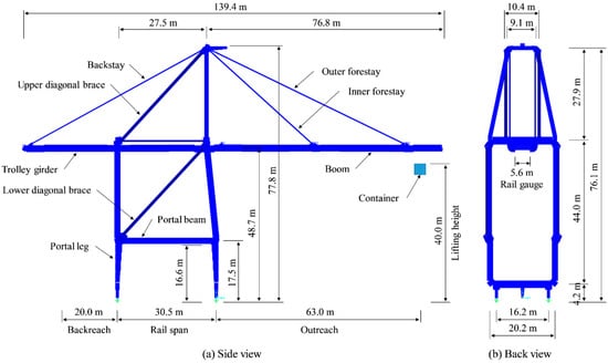
Figure 1.
Overall dimensions of a Korean A-frame container crane.
In South Korea, the seismic performance of the container crane has not been considered for most of the port design guidelines in the past, because South Korea was expected to be less severely affected by earthquakes. However, strong shaking occurred recently, i.e., the 5.4-magnitude Pohang earthquake on 15 November 2017 [4], and the 5.8-magnitude Gyeongju earthquake on 12 December 2016 [5], which damaged several buildings, port facilities, roads, and bridges. Thus, it is of utmost importance to consider the seismic analysis for a container crane to reduce the economic and human losses due to earthquake.
Historically, many ports have been partially destroyed by earthquakes, e.g., the port of Kobe (Japan) in 1995 [6], port in Port-au-Prince (Haiti) in 2010 [1], and port in Chile in 1985 [7], requiring a long time for repair and recovery. When a container crane completely collapses, it typically takes 12–24 months to purchase a new port crane [8]; thus, pre-defined damage levels and structural performance are necessary in the seismic performance evaluations of new and existing cranes to predict their risks. Fragility analysis is a key input parameter for the seismic risk assessment of a structural component or entire system, and enables the evaluation of the potential damage thresholds and specific repair models of a structural component in a system during a predefined intensity earthquake [1]. The fragility curve, which is usually assumed to be a cumulative distribution function (CDF) [9], was first applied to civil infrastructures in ATC-13 in the mid-1980s [10] and was later applied to many types of structures such as bridges [11,12], highways [13], buildings [14], tunnels [15,16], and ports [1,17]. Fragility assessment for the container crane has not been widely studied. A significant study was conducted by Kosbab et al. [1,18]. Three two-dimensional (2D) numerical models of American cranes, i.e., J100, LD100, and LD50, were considered with overall limit states obtained in terms of critical portal deformations. Based on previous experimental and numerical studies, hysteretic rotational springs were utilized to capture both elastic and inelastic behavioral features. In addition to earthquake excitation, fragility assessment owing to stochastic wind loading was also considered for container cranes [19].
In this study, a three-dimensional (3D) finite element (FE) model of a typical Korean container crane was used in the fragility analyses. The damage or limit states were defined in terms of portal drift using nonlinear static analysis with plastic hinges defined in compliance with ASCE/SEI 41 [20]. Nonlinear time-history analyses were applied while gradually increasing the earthquake intensity (IM). A set of 20 recorded and artificial ground motions per IM were matched to the Korean design response spectra [21]. The contacts between the crane’s toes and the wharf/rails were simulated by isolator elements of SAP2000 (a finite element software package of Computers and Structures Inc., Berkeley, California, United States), which allow capture of the uplift and derailment behavior. The rest of this paper is structured as follows: Section 2 introduces the methodology for the analytical fragility analysis and covers the procedure to obtain the research goal. Section 3 describes the time-history analyses using the 3D numerical model to develop the fragility curves. Section 4 presents the results of the analyses, and discusses the performance-based fragility curves. Finally, Section 5 concludes the paper.
2. Analytical Fragility
2.1. Methodology of Fragility Assessment
Fragility analyses, also known as fragility curves, are representations of conditional probability that indicate the probability of exceeding a pre-defined level of damage as subjected to an input seismic intensity parameter [12]. The fragility function represents the ability of a system to withstand a specified event, and can be expressed as
where P[LS|IM = x] represents the probability that a ground motion with IM = x causes the structure to collapse with a given pre-defined limit state (LS). IM can be expressed in terms of the peak ground acceleration/velocity/displacement or spectral acceleration at the fundamental period [9]. There are four common methods for fragility assessment: (1) professional judgement; (2) quasi-static and design code consistent analysis; (3) damage data associated with past earthquakes (the so-called empirical fragility analysis); and (4) numerical simulation of seismic responses based on structural dynamic analysis or the so-called analytical fragility analysis [22]. In the absence of adequate damage data, the empirical fragility curve will be inaccurate. Thus, an analytical fragility analysis in which the limit states are defined based on ASCE/SEI 41 [20] for steel building structure can be a suitable tool for assessing a container crane. The definition of limit states is discussed in detail in Section 2.3.
Increasing IM levels were generated to cover the entire range of each fragility curve. For each IM level, 20 ground motions created by matching the IM level with the design response spectra of the Korean Building Code (KBC) [21,23] were used as input parameters for the FE model. Time-history analyses were conducted to obtain the critical portal drift. Figure 2 illustrates the framework of this study.
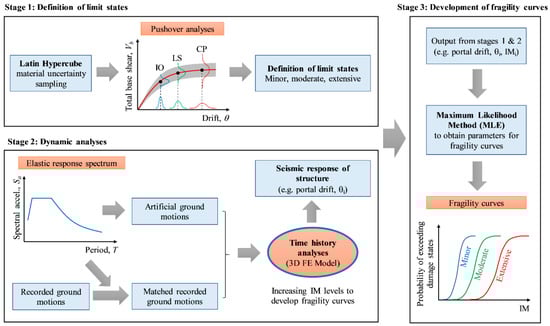
Figure 2.
Methodology of fragility curve development.
2.2. Selection of Seismic Demands
Based on the authors’ previous study [24], the sensitivity of a crane structure was analyzed and used for identifying the sources of uncertainty that are significant to the response of the structure. A series of random variables including ground motion intensity, ground motion profiles, mass, damping, and elastic modulus of steel, were considered. The results demonstrated that among all the sources of uncertainty considered, the ground motion intensity and profile played the most important role in the overall response of the container crane in terms of portal drift. In addition, the elastic modulus was recommended to be considered as a source of uncertainty in a seismic analysis. Thus, to minimize the computational cost, the ground motion intensity and profile were considered as the demand randomness, and the elastic modulus of steel was considered as the capacity randomness of the container crane. Other uncertain parameters in the finite element analysis were evaluated to be deterministic at their mean/median values.
To consider the site conditions where the crane was located, many boreholes were drilled to investigate some major physical characteristics of the ground, especially the shear wave velocity (vs) of the top 30 m from the ground surface. The report revealed that the minimum and maximum of vs were approximately 247 and 447 m/s, respectively, indicating that the soil classes ranged from S2 to S3 according to the KBC, as presented in Table 1.

Table 1.
Site classification (soil classes) of Korean Building Code [21].
For the crane’s site, seismic zone I (with a seismic zone factor of Z = 0.11× g) was considered. By assuming a return period of 500 years as recommended for port structures, that the crane works under the Immediate Occupancy (IO) performance level [23], and the chosen soil class is S3, the 1.5% damping horizontal acceleration response spectrum was developed, as illustrated in Figure 3a.
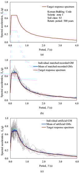
Figure 3.
(a) Target response spectrum (1.5% damping); (b) matched recorded response spectra; and (c) artificial response spectra. GM: Ground Motion.
Ten recorded ground motions (denoted as RGMs) were selected to consider the effect of the realistic ground motion profile, as presented in Table 2. Then, a spectrum matching process was conducted on the design response spectrum illustrated in Figure 3b, to generate 10 design spectrum-matched ground motions, as depicted in Figure 4a. The reason for using the spectrum matching technique is to reduce the variability (jaggedness) observed in the acceleration spectra for individual ground motions [25].
Table 2.
Original recorded ground motions (unmatched).
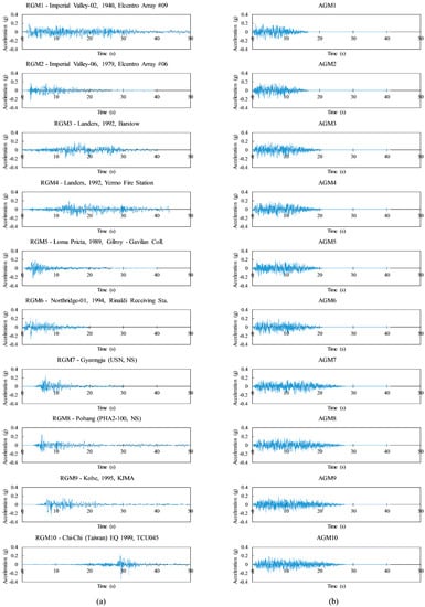
Figure 4.
(a) Matched recorded ground motions; and (b) artificial ground motions.
To ensure that the ground motions had a number of peaks of similar amplitude, 10 artificial ground motions (denoted as AGMs) were generated based on the prescribed response spectrum of Figure 3a. The QuakeGem program was used [26], which is dependent on the spectral-representation-based simulation algorithm proposed by Deodatis in 1996 [27,28], with a filtered white noise signal by three different trapezoidal envelope functions. The trapezoidal functions include the rise time (1–2 s), vibration duration (8–14.5 s), and descent time (17–28 s). Figure 3c and Figure 4b depict 10 individual artificial response spectra and the corresponding artificial time-history accelerations, respectively.
2.3. Damage States for Container Crane
For the randomness in a structural capacity, the uncertainty of the overall stiffness of the structure may mainly originate from the structure’s geometric dimensions and material properties. In this study, with the assumption that the steel plates were perfectly manufactured, the elastic modulus was the only parameter to be considered as a normal distribution random variable with a mean value of 200 GPa and coefficient of variation (COV) of 0.06 [24]. A nonlinear static analysis was then performed to discover the capacity behind the elastic states. The limit states obtained by a pin-based pushover can be applied for comparison with the response obtained from a dynamic analysis because the capacity of the structure is load-independent [1]. The force-displacement curve was obtained by gradually increasing the lateral force assigned at the boom level of the crane. This approach was conducted successfully in the authors’ previous study [29]; However, all input parameters were used in the previous study as best estimates (mean/median values), without considering the uncertainty of the input values to the response of the structure.
To assess the uncertainty in the input value of the structural capacity, 50 input cases of the elastic modulus values were generated by Latin Hypercube Sampling (LHS). This was accomplished to reduce the computational effort in comparison with Monte Carlo Simulation (MCS) sampling because of the stratified technique for the input probability distributions of the LHS method [30]. Correspondingly, 50 different pushover analyses were conducted on finite element models with uncertain variables of the elastic modulus to identify the limit states of the damage based on predefined plastic hinges of ASCE/SEI 41 [20]. For the FE model, the structural components were modeled with one-dimensional beam-column finite elements. Thus, the concentrated (or lumped) plasticity approach was applied for the nonlinear material response. In this approach, the constitutive laws are expressed in terms of moment-rotation (M-θ) relationships of the cross section of interest. The M-θ relationship of each section can be defined assuming a backbone as indicated in ASCE/SEI 41. The lumped plasticity approach is more robust and reduces the computational cost. However, it restricts the inelastic deformations to prespecified regions of small length. In this study, the three predefined performance-based damage levels of ASCE/SEI 41, i.e., immediate occupancy (IO), life safety (LS), and collapse prevention (CP), are assumed as minor, moderate, and extensive damage states, respectively, in terms of the portal drift of the container crane. This is depicted in Figure 5, while Table 3 summarizes the corresponding average values. Table 3 is useful for the preliminary design of a 30.5-m-gauge container crane. For example, if an elastic state is expected for designing a 30.5-m-gauge crane with structural similarity, its portal drift, defined as the drift angle between the leg base and the portal beam (see Figure 1), should be less than the minor state listed in Table 3. The values listed in Table 3 are crucial for developing the fragility curves.
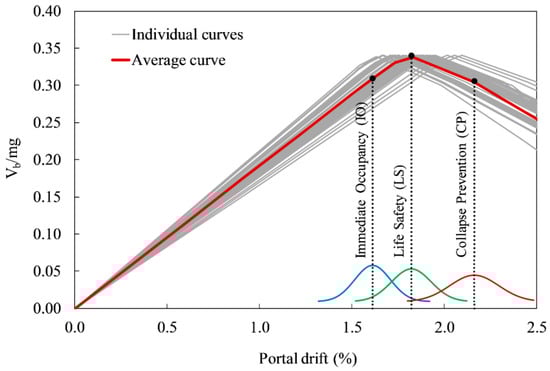
Figure 5.
Pushover curves for the 50 random cases generated by Latin Hypercube sampling.
Table 3.
Limit states in terms of portal drift.
3. Dynamic Analysis of Container Crane Coupled with Uplift and Derailment
3.1. Nonlinear Time-History Analyses
In this study, a direct-integration nonlinear time-history analysis was used in which the Hilber–Hughes–Taylor (HHT) method was applied to improve the numerical dissipation of the time integration algorithm. The parameters of the HHT method were γ = 0.5, β = 0.25, and α = 0 (assuming that the formulation will be identical to the average acceleration method) [31,32]. The 3D finite element model of the Korean container crane is composed of 9916 elements, whereas four friction isolator elements are used to simulate the behavior between wharf and crane’s toes. Most of the structural components of the crane were made of stiffened hollow box sections. The properties of materials comply with the Japanese Industrial Standards (JIS) including JIS-SM490Y (for hollow box sections and wide-flange shapes) and JIS-STK490 (for steel tubes of diagonal braces), as summarized in Table 4.
Table 4.
Properties of materials.
To develop the fragility curves, a total of 20 recorded and artificial horizontal ground motions matched for the design spectrum as mentioned in Section 2.2 were used under 23 IM levels ranging from 0.17 to 0.75× g. Thus, 460 ground motions were applied as input data for the seismic demand. For container cranes, the impact of the vertical ground motion on the response of the crane was approximately 0.1% of the portal drift for the level of excitation, Sa (0.3 s) < 0.5× g [1]. The effect of the vertical ground motion should be analyzed on an entire complex soil-structure interaction and quay wall system [24]. In this study, a simpler model was used to reduce the cost and time required. Thus, the vertical ground motions were neglected.
The IM of this research is the spectral acceleration at the fundamental natural period of the container crane, Sa (T = 1.68 s). The fundamental period of this study (applying a friction isolator element at the base) was found to be longer than those obtained from our previous studies using the pin-support and gap element [24,29]. Zero-length link elements of SAP2000 (or a friction isolator element as above-mentioned) were assigned to the model’s toes to simulate the contact friction, enabling both uplift and derailment, because the behavior of these elements was similar to the real interaction between the crane wheel and the rail during the operation of the crane. The uplift and derailment behaviors changed the horizontal displacement of the entire structure; thus, the corresponding fragility curves were different from those obtained from other boundary conditions such as pin or gap elements [29,33]. The friction isolator element exhibited a vertical behavior similar to that of the gap element (see [24]); However, the gap element did not remove itself from the horizontal direction during uplift. The friction isolator element could solve the horizontal force capacity throughout the compressive vertical force and frictional coefficient (μ). Here, the frictional coefficient (μ is assumed to be 0.75) ignored the difference between static and kinetic friction. For the friction isolator element, both the horizontal and vertical reactions of the legs will reach zero if the legs have uplift and derailment events [33]. In this study, the stiff spring constant (kk) of the friction isolator element is assumed to be 43,782 kN/cm [24].
Based on both physical test and analytical model from previous studies, the seismic response of the container crane over time can be divided into three stages [1,6,34], as depicted in Figure 6: (a) the structure is shaken owing to low seismic load (so-called swaying). (b) With a higher seismic load, the landside legs are uplifted and derailed (lateral translation) when the total gravity load is transferred to the waterside legs owing to the considerable reduction in the axial load on the landside legs. As a result, when the load is added to the waterside legs due to the uplift of the landside legs [1], plastic hinges can occur on the waterside legs. Finally, (c) the landside legs land inside the rail, resulting in a residual inward displacement of each leg. In this stage, plastic hinges may also develop on the landside legs. The first occurrence of a plastic hinge can be at either the waterside or landside legs, which can depend on the design strength of the portal frame, ground motion profile and intensity, direction of the earthquake, or friction between the ground/rails and the crane wheels. The torsional flexibility makes a negligible contribution to the portal flexibility even with significant seismic excitation. This has been verified by many studies using push-twist analysis for the A-frame container crane [1,29]. Therefore, in this study, the torsional effect was ignored when evaluating the seismic performance of the portal crane response.
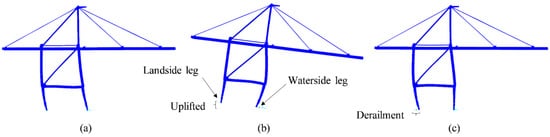
Figure 6.
Failure modes of container crane under seismic loading: (a) swaying; (b) uplifted legs with/without derailment; and (c) permanent derailment and remaining deformation.
Figure 7 illustrates an example of the seismic response of a crane subjected to artificial ground motion (AGM8) with Peak Ground Acceleration(PGA) of 0.51 g (equivalent to a scale factor of 3.0 in comparison with the AGM8 depicted in Figure 4b), considering both the uplift and derailment behaviors. There are four occurrences of uplift at the landside leg. The first uplift occurred at 3.24 s, reaching its maximum value of 0.04 cm at 3.3 s. Concurrently, it was derailed by as much as 10.4 cm inward at the rail. The second, third, and fourth occurrences of the maximum uplifts were 0.5, 0.1, and 0.9 cm at 4.93, 6.94, and 8.64 s, corresponding to the total permanent derailments of 34.5, 39.2, and 52.0 cm. In this study, the uplift behavior is related to the redistribution of the load. The uplift is defined by two conditions, as mentioned in the study proposed by Tran et al. [29], in which both vertical displacement and the reaction of the uplifted leg are equal to or larger than zero. In particular, Figure 7b illustrates the four occurrences of uplifting, corresponding to four occurrences of vertical reaction reduced to zero in Figure 7c. Both waterside legs and one landside leg of the crane in this example drift over the limit state of collapse prevention, indicating a potential overturning collapse toward the sea. The analyses of this study ignore the lateral restraint provided by a small flange on each wheel. Thus, the derailment is controlled by the weight of the crane, and the friction between the crane’s toes and the ground/rail.
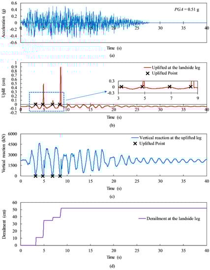
Figure 7.
Example of uplift and derailment behaviors of a container crane subjected to artificial ground motion (AGM)2: (a) ground motion with PGA of 0.51× g; (b) uplift of landside legs; (c) vertical reaction of landside legs at time of uplifting; and (d) derailment of landside legs.
3.2. Probability of Exceedance of Uplift
Based on the above-mentioned definition of uplift behavior, uplift and derailment are considered to be independent limit states because they can occur with or without structural damage. This is discussed in detail when the uplift curve is considered together with the IO, LS, and CP curves in the following sections. The fragility curve of excessive uplift was constructed as the principle of Equation (1) and is detailed in Section 4. Fourteen IM levels were generated ranging from 0.17 to 0.61× g, in which each IM level is illustrated as a blue dot in Figure 8 and includes 20 different ground motions. The probability of exceeding uplift under different IM levels was fitted by a log-normal CDF depicted as the red solid line in Figure 8. The median and standard deviation of ln(IM) are 0.31 and 0.248× g, respectively.
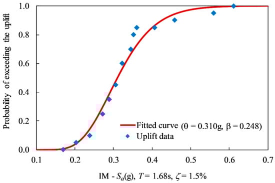
Figure 8.
Probability of exceeding uplift.
4. Performance-Based Fragility Curves
As mentioned previously, the log-normal CDF was used to define the fragility function [9,35,36]. Thus, Equation (1) can be expressed as follows:
where, is the standard normal cumulative distribution function, and θ and β are the median and standard deviation of ln(IM), respectively. At each IM = xj, the structural analyses produce some number of collapses out of the total number of ground motions. The probability of observing collapses or no collapses is given by the binomial distribution. Hence, the MLE function is:
where, pj represents the probability that a ground motion with IM = xj causes the collapse, zj is the number of collapses out of nj ground motions, and m represents the number of the IM level. In order to perform this maximization, Equation (2) is substituted into Equation (3), so the fragility parameters are explicit in the likelihood function:
The parameters that maximize this likelihood function also maximize the log of the likelihood. The “” notation denotes the estimate of a parameter:
Figure 9 depicts the three fragility curves built from the definition of Table 3. As a result, the median values of IM (in terms of PGA) were 0.487, 0.521, and 0.557× g for the minor, moderate, and extensive limit states, respectively. Correspondingly, the standard deviations of ln(PGA) were 0.232, 0.235, and 0.240× g for the minor, moderate, and extensive states, respectively. To consider the IM in terms of the spectral acceleration during period T of 1.68 s and damping ratio ζ of 1.5%, the median values of Sa were 0.387, 0.413, and 0.442× g for the minor, moderate, and extensive states, corresponding to the log-standard deviations of 0.232, 0.235, and 0.240× g. The standard deviations indicate the slopes of the fragility curves, and increase as the performance levels shift from the minor to extensive damage state.
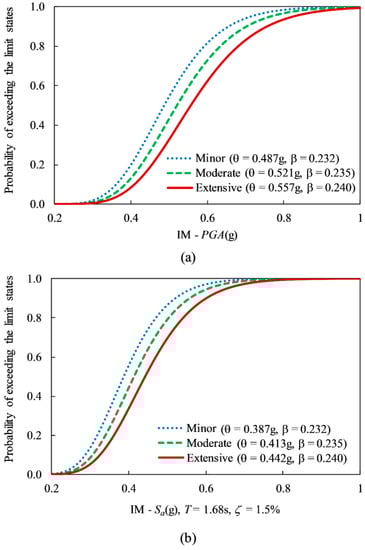
Figure 9.
Fragility curves for minor, moderate, and extensive limit states; (a) IM is PGA; and (b) IM is Sa (T = 1.68 s, ζ = 1.5%).
When an uplift coupled with derailment occurs, the crane is repositioned and its functionality restored after landing inside the rails. Failure can occur before or after the uplift threshold depending on the capacity of each crane. In this analysis, failure occurred after the uplift threshold, and thus the probabilities of exceeding IO, LS, and CP performance levels must be considered with the uplift and derailment behavior, as shown in Figure 10. At the same IM level, e.g., at Sa = 0.387× g, it can be clearly seen that the 50% probability of exceeding the IO level will be coupled with a probability of approximately 80% of exceeding the uplift. Similarly, a 50% probability of exceeding LS (Sa = 0.413× g) and CP (Sa = 0.442× g) levels will occur with an approximately 85% and 90% probability of uplift, respectively.
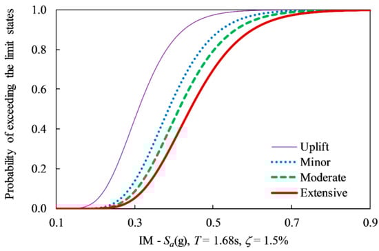
Figure 10.
Fragility curves for uplift, minor, moderate, and extensive limit states.
Based on the proposed fragility curves as illustrated in Figure 9 and Figure 10, the vulnerability assessment can be predicted as in the example in Table 5 for five different expected seismic levels with a structure of 1.5% damping located on soil S3. The values presented in Table 5 are the probabilities of exceeding damage levels for 200, 500, 1000, 2400, and 4800 average years of return period for the earthquake. These are equivalent to a 10% probability of occurrence within 20, 50, 100, 250, and 500 years of the life span of the structure, as recommended in the KBC. Table 5 can serve as a set of recommendations for port owners who wish to select a suitable level of risk for their existing cranes, and an appropriate retrofit plan if the cranes suffer an earthquake event in the future. For example, if the owners expect a minor performance level with seismic Level I for their existing cranes at a Korean port [23], and the selected return period of an earthquake is 2400 years, then the probability of exceeding minor damage to the crane structures or facilities is approximately 12.4% under the average spectral acceleration Sa of 0.3× g. Simultaneously, the probability of exceeding an uplift is approximately 42.5%. On the other hand, assuming that the earthquake has a return period of 1000 years, the probability of exceeding the minor damage of the structure is just only approximately 0.6%. However, business operations can be interrupted towing to the 7.5% probability of uplift with derailment, because of the operational downtime required for jacking and repositioning the wheels of the crane back to the rail.
Table 5.
Example of probability of exceeding damage levels (unit %) for five seismic levels (soil S3) of Korean port design requirements.
Figure 11 illustrates the fragility curves that were plotted with four different natural periods of the crane to serve as a preliminary design, and to estimate the probability of exceedance for an expected limit state. Based on Figure 11, designers or port owners can predict the probability of exceeding the limit states of container cranes by calculating a linear interpolation of the fundamental periods ranging from 0.5 to 2.0 s. Table 6 lists the parameters of these fragility curve models. It is assumed that the standard deviation of ln(Sa) is similar to those obtained from Section 4 (see Figure 9 as well).
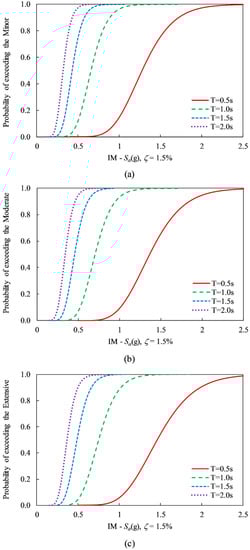
Figure 11.
Fragility curves with different periods of container crane for (a) minor damage state; (b) moderate damage state; and (c) extensive damage state.
Table 6.
Median and standard deviation of ln(Sa).
5. Conclusions
This study focused on the time-history acceleration analysis of a typical modern jumbo container crane, as well as the methodology of the fragility curve development. The methodology can be applied to predict the probability of exceeding the limit states, based on predefined damage criteria obtained from the combination of a pushover analysis and Latin Hypercube sampling. In addition, the uplift behavior coupled with derailment, which indicates the realistic interaction between the crane toes and the ground/rails, was studied in detail to construct the corresponding fragility curves. The uncertainties of the demand and capacity of the structure were considered, including the elastic modulus, ground motion profile, and intensity.
In this study, the uplift occurred before other damage states. For the container crane of this study, a 50% probability of exceeding the minor damage state was coupled with a probability of approximately 80% of excessive uplift. Similarly, a 50% probability of exceeding the moderate and extensive damage levels occurred with a probability of uplift of approximately 85% and 90%, respectively. The longer the natural period of a container crane, the higher the probability of occurrence of the uplift coupled with derailment. This interrupts business operations, owing to the operational downtime required for jacking and repositioning the crane back to the rail. Furthermore, this study presented fragility curves that were developed for different natural structural periods. These curves can assist port stakeholders/designers considering the risk of their container cranes at an expected performance level.
Author Contributions
Conceptualization, J.H. and Q.H.T.; Methodology, J.H.; Software, Q.H.T., N.S.D. and V.H.M.; Validation, Q.H.T. and J.-H.A.; Formal Analysis, Q.H.T. and N.S.D.; Resources, J.H.; Data Curation, Q.H.T. and N.S.D.; Writing-Original Draft Preparation, Q.H.T. and J.H.; Writing-Review & Editing, J.H. and J.-H.A.; Supervision, J.H.
Acknowledgments
This research was a part of the project entitled ‘Development of performance-based seismic design technologies for advancement in design codes for port structures’, funded by the Ministry of Oceans and Fisheries, Korea; and was also supported by the Basic Science Research Program through the National Research Foundation of Korea (NRF), funded by the Ministry of Education (2017R1D1A3B03032854).
Conflicts of Interest
The authors declare no conflict of interest.
References
- Kosbab, B.D. Seismic Performance Evaluation of Port Container Cranes Allowed to Uplift; Georgia Institute of Technology: Atlanta, GA, USA, 2010. [Google Scholar]
- Soderberg, E.; Hsieh, J.; Dix, A. Seismic Guidelines for Container Cranes. In Proceedings of the TCLEE 2009: Lifeline Earthquake Engineering in a Multihazard Environment, Oakland, CA, USA, 28 June–1 July 2009. [Google Scholar]
- Bhimani, A.; Jordan, M.A. A few facts about jumbo cranes. In Proceedings of the TOC Americas in Panama, Panama City, Panama, 3 December 2003. [Google Scholar]
- Kim, H.-H.; Ree, J.-H.; Kim, Y.; Kim, S.; Kang, S.-Y.; Seo, W. Assessing whether the 2017 Mw 5.4 Pohang earthquake in South Korea was an induced event. Science 2018, 360, 1007–1009. [Google Scholar] [CrossRef] [PubMed]
- Kim, S.-K.; Lee, J.-M. Probabilistic seismic hazard analysis using a synthetic earthquake catalog: Comparison of the Gyeongju City Hall site with the Seoul City Hall site in Korea. Geosci. J. 2017, 21, 523–533. [Google Scholar] [CrossRef]
- Kanayama, T.; Kashiwazaki, A. An Evaluation of Uplifting Behavior of Container Cranes under Strong Earthquakes. Trans. Jpn. Soc. Mech. Eng. 1998, 64, 100–106. (In Japanese) [Google Scholar]
- PIANC. Seismic Design Guidelines for Port Structures; A.A. Balkema: Brussels, Belgium, 2001. [Google Scholar]
- Vuojolainen, M.; Van Der Waal, J. A Longer Lift for your Port Cranes; Kalmar: Helsinki, Finland, 2015. [Google Scholar]
- Baker, J.W. Efficient analytical fragility function fitting using dynamic structural analysis. Earthq. Spectra 2015, 31, 579. [Google Scholar] [CrossRef]
- Applied Technology Council. ATC-13, Earthquake Damage Evaluation Data for California; FEMA: Redwood City, CA, USA, 1985. [Google Scholar]
- Shinozuka, M.; Feng, M.Q.; Kim, H.-K.; Kim, S.-H. Nonlinear static procedure for fragility curve development. J. Eng. Mech. 2000, 126, 1287–1295. [Google Scholar] [CrossRef]
- Padgett, J.E.; DesRoches, R. Methodology for the development of analytical fragility curves for retrofitted bridges. Earthq. Eng. Struct. Dyn. 2008, 37, 1157–1174. [Google Scholar] [CrossRef]
- Pitilakis, K. D3.7—Fragility Functions for Roadway System Elements; Norwegian Geotechnical Institute (NGI)-Seventh Framework Program: Oslo, Norway, 2009. [Google Scholar]
- Ramamoorthy, S.K.; Gardoni, P.; Bracci, J.M. Probabilistic Demand Models and Fragility Curves for Reinforced Concrete Frames. J. Struct. Eng. 2006, 132, 1563. [Google Scholar] [CrossRef]
- Huh, J.; Tran, Q.H.; Haldar, A.; Park, I.; Ahn, J.-H. Seismic Vulnerability Assessment of a Shallow Two-Story Underground RC Box Structure. Appl. Sci. 2017, 7, 735. [Google Scholar] [CrossRef]
- Argyroudis, S.A.; Pitilakis, K.D. Seismic fragility curves of shallow tunnels in alluvial deposits. Soil Dyn. Earthq. Eng. 2012, 35, 1–12. [Google Scholar] [CrossRef]
- Heidary-Torkamani, H.; Bargi, K.; Amirabadi, R.; McCllough, N.J. Fragility estimation and sensitivity analysis of an idealized pile-supported wharf with batter piles. Soil Dyn. Earthq. Eng. 2014, 61–62, 92–106. [Google Scholar] [CrossRef]
- Kosbab, B.; DesRoches, R.; Leon, R. Seismic Fragility of Jumbo Port Container Cranes. In Proceedings of the 12th Triannual International Conference on Ports, Jacksonville, FL, USA, 25–28 April 2010. [Google Scholar]
- Gur, S.; Ray-Chaudhuri, S. Vulnerability assessment of container cranes under stochastic wind loading. Struct. Infrastruct. Eng. 2014, 10, 1511–1530. [Google Scholar] [CrossRef]
- American Society of Civil Engineers. Seismic Evaluation and Retrofit of Existing Buildings; ASCE/SEI 41; American Society of Civil Engineers: Reston, VA, USA, 2013. [Google Scholar]
- Architectural Institute of Korea. Korean Building Code; Architectural Institute of Korea: Seoul, Korea, 2016. [Google Scholar]
- Shinozuka, M.; Feng, M.Q.; Kim, H.; Uzawa, T.; Ueda, T. Statistical Analysis of Fragility Curves; University of Southern California: Los Angeles, CA, USA, 2001. [Google Scholar]
- Kim, I. Seismic Design and Performance Objectives of Civil Facilities. Mag. KSCE 2017, 65, 20–25. [Google Scholar]
- Tran, Q.H.; Huh, J.; Nguyen, V.B.; Kang, C.; Ahn, J.-H.; Park, I.-J. Sensitivity Analysis for Ship-to-Shore Container Crane Design. Appl. Sci. 2018, 8, 1667. [Google Scholar] [CrossRef]
- Whittaker, A.; Atkinson, G.; Baker, J.; Bray, J.; Grant, D.; Hamburger, R.; Haselton, C.; Somerville, P. Selecting and Scaling Earthquake Ground Motions for Performing Response-History Analyses; Grant/Contract Reports (NISTGCR)-11-917-15; National Institute of Standards and Technology: Gaithersburg, MD, USA, 2011.
- Kim, J.M. QuakeGem—Computer Program for Generating Multiple Earthquake Motions; Chonnam National University: Jellanam-do, Korea, 2007. [Google Scholar]
- Deodatis, G. Non-stationary Stochastic Vector Processes: Seismic Ground Motion Applications. Probabilistic Eng. Mech. 1996, 11, 149–168. [Google Scholar] [CrossRef]
- Deodatis, G. Simulation of Ergodic Multivariate Stochastic Processes. J. Eng. Mech. 1996, 122, 778–787. [Google Scholar] [CrossRef]
- Tran, Q.H.; Huh, J.; Nguyen, V.B.; Haldar, A.; Kang, C.; Hwang, K.M. Comparative Study of Nonlinear Static and Time-History Analyses of Typical Korean STS Container Cranes. Adv. Civ. Eng. 2018, 2018, 2176894. [Google Scholar] [CrossRef]
- Iman, R.L.; Conover, W. Small sample sensitivity analysis techniques for computer models with an application to risk assessment. Commun. Stat.-Theory Methods 1980, 9, 1749–1842. [Google Scholar] [CrossRef]
- Wilson, E. Three-Dimensional Static and Dynamic Analysis of Structures: A Physical Approach with Emphasis on Earthquake Engineering; CSI: Berkeley, CA, USA, 2002. [Google Scholar]
- Computers and Structures Inc. Linear and Nonlinear Static and Dynamic Analysis and Design of 3D Structures: Basic Analysis Reference Manual for SAP2000; CSI: Berkeley, CA, USA, 2006. [Google Scholar]
- Huh, J.; Nguyen, V.B.; Tran, Q.H.; Ahn, J.-H.; Kang, C. Effects of Boundary Condition Models on the Seismic Responses of a Container Crane. Appl. Sci. 2019, 9, 241. [Google Scholar] [CrossRef]
- Kourkoulis, R.; Gelagoti, F.; Loli, M. Seismic Vulnerability of Container Cranes: The Role of Soil-Structure Interaction in Jeopardising Their Operability. In Proceedings of the SECED 2015 Conference: Earthquake Risk and Engineering towards a Resilient World, Cambridge, UK, 9–10 July 2015. [Google Scholar]
- Ibarra, L.F.; Krawinkler, H. Global Collapse of Frame Structures under Seismic Excitations; PEER Center; University of California: Berkeley, CA, USA, 2005. [Google Scholar]
- Lee, T.-H.; Mosalam, K.M. Probabilistic Seismic Evaluation of Reinforced Concrete Structural Components and Systems; University of California: Berkeley, CA, USA, 2006. [Google Scholar]
© 2019 by the authors. Licensee MDPI, Basel, Switzerland. This article is an open access article distributed under the terms and conditions of the Creative Commons Attribution (CC BY) license (http://creativecommons.org/licenses/by/4.0/).