An Integrated Computational Approach for Seismic Risk Assessment of Individual Buildings


1
Department of Civil Engineering, Universidade do Algarve, Faro 8005-139, Portugal
2
CIMA—Centre for Marine and Environmental Research, UAlg, Faro 8005-139, Portugal
Appl. Sci. 2019, 9(23), 5088; https://doi.org/10.3390/app9235088
Submission received: 26 October 2019
/
Revised: 14 November 2019
/
Accepted: 22 November 2019
/
Published: 25 November 2019
(This article belongs to the Special Issue Evaluation and Mitigation of Seismic Risk for Existing Buildings, Structures, and Infrastructures)
Abstract
:The simultaneous assessment of a great number of buildings subjected to different ground motions is a very challenging task. For this reason, a new computational integrated approach for seismic assessment of individual buildings is presented, which consists of several independent computer objects, each having its own user interface, yet being totally interconnectable like in a puzzle. The hazard module allows considering a code-based response spectrum or a predicted response spectrum for a given earthquake scenario, which is computed throughout the resolution of an optimization problem. The vulnerability of each building is assessed based on structural capacity curves. Damage is evaluated using an innovative proposal, which is to use what was called a performance curve associated with a capacity curve. This curve reproduces the percentage of a given response spectrum corresponding to a performance point for each displacement value of a capacity curve. Therefore, it becomes possible to do a very fast association of any limit state to a percentage of a seismic action. This approach was implemented in the PERSISTAH software, and the result outputs can be exported, instantaneously, to the Google Earth software throughout the creation of a kml file, or to MS Excel.
1. Introduction
The seismic risk assessment of existing buildings is a very important issue, particularly when managing the seismic safety of a school campus. It is well known that schools are places normally with many children taking classes in several different buildings that compose a campus, which may present many different structural systems and construction ages. So, the context of seismic risk assessment of individual school building is especially important due to the high concentration of young people normally found in such facilities. The collapse of a school building during the 2002 Molise Earthquake (Italy), killing many students and a teacher [1], where the site effects also seem to have played an important role in the damage [2], is a good example of the importance of an accurate seismic risk assessment of existing school buildings in order to identify the most problematic cases, namely for retrofitting purposes. More recently, many Italian school buildings were also damaged after the 2016 Central Italy earthquake sequence [3], highlighting this issue. In this context, it is important to develop seismic assessment methods to carry out these types of studies at a large scale, while considering the specific characteristics of each building, and trying to increase the precision of results.
Because of this issue’s importance, the PERSISTAH project aims to assess the seismic risk of primary school buildings in the Algarve (Portugal) and Huelva (Spain) regions [4] by developing a dedicated software for its purpose.
Presently, there are many proposals for carrying out the seismic assessment of individual school buildings. Many recent studies dealing with school buildings have adopted nonlinear structural analysis methods. In some of those studies, authors have adopted nonlinear dynamic analysis (NDA) [5,6], which is probably the most accurate approach, namely the incremental dynamic analysis (INDA) [7,8]. However, this requires much computer effort. Nonlinear static analysis (NSA) is a very popular method of analysis, and is a more simplified and fast approach that has also been used to assess school buildings [9,10,11,12]. The results obtained with these two approaches are different [7], so the option of selecting one of these two nonlinear analysis methods must be carefully evaluated regarding the precision of the results and the speed of the process.
The first NSA was proposed in the 1970s as a fast way of carrying out seismic vulnerability assessments, but the capacity spectrum method (CSM) designation was only introduced during the 1990s [13]. CSM is an NSA approach used worldwide and was adopted by the ATC-40 [14], it being the nonlinear inelastic behaviour of a structural system obtained by applying effective viscous damping values to the linear elastic response spectrum. Another NSA approach is the N2 method, with the first formulation developed in the late 1980s, and later reformulated at the end of the 1990s [15]. In this method, inelastic spectra are used [16] instead of the approach presented in the CSM. The N2 is the NSA approach that is presented in the Eurocode 8 (EC8) [17]. According to these approaches, the structural performance point (the target displacement) is the interception between the structural capacity and the seismic demand.
The development of software for the seismic risk assessment is an important but complex task. At the present time, there are many modern seismic risk assessment tools developed by different research teams around the world [18,19,20,21] that have been used for many purposes; in particular, some of them are being used in the context of civil protection mechanisms. These tools normally present different modules related to the seismic risk definition (Figure 1); in particular, they might have a hazard analysis module, a vulnerability assessment module, a database module (exposure) and an output module where results can be exported to a GIS software (loss maps). In Table 1, several seismic risk assessment (SRA) tools developed worldwide are listed.
In current SRA tools (Table 1), there are many options to define the ground-motion parameters in the hazard module, which can result from a deterministic analysis, a probabilistic analysis, a code-based seismic action or simply using real earthquake records. For the deterministic earthquake scenario option, ground-motion prediction equations (GMPEs) are usually adopted to compute an intensity, or the peak ground acceleration (PGA), or even an entire response spectrum and, as expected, the results precision normally increases with the complexity of the approach. There are also many possibilities to establish the earthquake source: A simple point source, a line source or a 3D fault plane. The site effects are also normally considered in SRA tools.
In vulnerability modules, the seismic performance of a building can be computed through the use of empirical or mechanical methods. The macro-seismic approach is one of the adopted empirical procedures that are used in large scale studies. This approach is normally used together with earthquake intensities. The most common mechanical approaches that are implemented in vulnerability modules of SRA tools are NSA approaches, like the CSM method or the N2 method.
The databases of elements exposed to seismic risk may be composed by individual buildings (the most accurate approach), or by area units with several buildings.
Damage is usually determined based on fragility curves, and losses are normally computed as a function of damage probability.
More than a description of a developed software, this paper is about a proposal of a new approach to develop SRA tools. This new approach was implemented in the PERSISTAH software, aiming at the SRA of school buildings, individually, in order to rank them for retrofitting purposes.
2. The SRA Proposed Approach
As presented in Table 1, there are many different SRA tools already developed worldwide, many of them available as freeware software, and some of them are even open-source tools. So, the development of new software could be considered a waste of time, unless some new developments were introduced, to account for the individual characteristics of school buildings, for example.
The main idea of the proposed approach was to transform some already developed computer routines into a set of independent computer objects that are totally interconnectable with each other. With this approach, it is possible to create new computer tools just by assembling a set of independent computer objects. These objects were obtained by dismembering the SIMULSIS [44,45] and the EC8spec [46] software, namely for the creation of the hazard and vulnerability modules.
In the PERSISTAH software, three modules were implemented: (1) The school database module (the exposure module), which consists of a computer object specifically developed for the PERSISTAH project, with all the information about the school buildings like general characteristics of the buildings, namely the geographical coordinates and some photos of the buildings; (2) the seismic action module (the hazard module), where a code-based seismic action (an EC8-type response spectrum) or an earthquake scenario can be selected, through the use of several independent computer objects developed for that task, which are also shared with other developed software (like the new versions of the SIMULSIS and EC8spec software); and (3) the damage assessment module, which is able to evaluate the seismic behaviour of an individual building. The capacity curve computer object (the vulnerability model) is used by the school database module and by the damage assessment module for the seismic assessment of each building. NSA methods were adopted for damage evaluation, namely the CSM and the N2 method, together with the use of fragility curves.
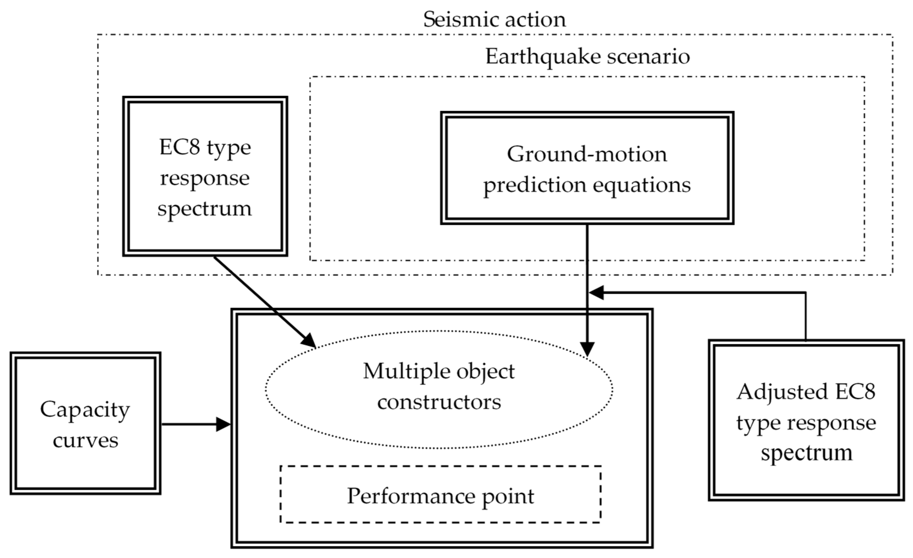
This approach leads to a very complex programming task, because, when developing an object, it is necessary to figure out which functions will be provided for the other objects. This paper will only focus on the last two modules, which are not specific for the PERSISTAH project, so it can be replicated for other tasks. Figure 2 presents the global scheme of analysis, which will be described in detail in the following sections. Each box of the figure is a different computer object. Each computer object has its own independent input/output user interface, where all the text is written in three different languages: Portuguese, Spanish and English. This means that all the developed computer objects can be used in the future to create new software, just like a puzzle, to be used in different regions of the world were these languages are currently spoken. All the computer code was developed in Object Pascal (Delphi).
3. Seismic Action
3.1. EC8-Type Response Spectrum
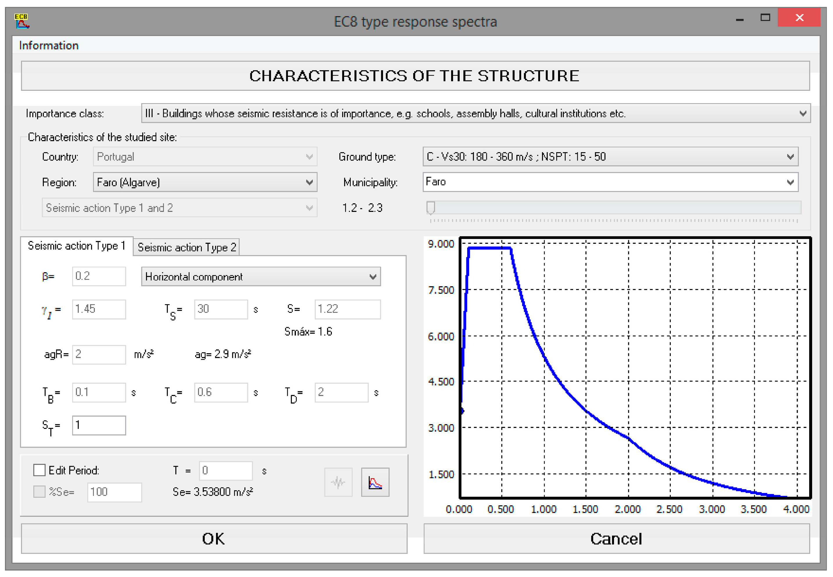
An object class was developed to deal with the EC8-type response spectrum (Figure 3). Then, it was possible to create several sub-classes (for each country/region), where all the specific values are defined, namely by municipality. In the context of the PERSISTAH software, two sub-classes were created: One for all Portuguese regions; and another only for the Huelva region (Spain). The great advantage of this approach is that the damage assessment module will always call the same computer routines, no matter the region where the building is located, simplifying this task.
For the PERSISTAH objectives, this computer object is important mainly to rank the school buildings for retrofitting purposes, based on the seismic security level of each individual building in accordance with the official seismic hazard of each country. This functionality can also be very useful to compare the seismic action proposed by different national codes in the borders of neighbouring countries, as is the case of Portugal and Spain.
3.2. Earthquake Scenario
This module allows to predict the structural seismic response of an individual building when subjected to a given earthquake scenario, and is composed of four different computer objects, (1) deals with all the basic characteristic of an earthquake (event magnitude, date, hour, epicentre coordinates, focus depth, etc.); (2) deals with the seismic sources (type of fault, azimuth, dip, etc.); (3) deals with the GMPEs, which compute a response spectrum for a given site, earthquake location and type of seismic source; and (4) is an object that fits a EC8-like response spectrum to the values obtained throughout the GMPEs.
3.2.1. Ground-Motion Prediction Equations
It is frequent to use GMPEs to assess the effects of earthquakes, which are also usually designated as attenuation laws. Normally, GMPEs are functions of the type of seismic fault (a strike-slip fault, a normal fault or a reverse fault), earthquake magnitude (M), a distance to the earthquake and the local geological characteristics of the studied site.
The result of the GMPEs may be an earthquake intensity, the PGA or some spectral coordinates of a response spectrum. In the proposed approach, only the latter GMPEs were implemented in the developed software. Moreover, three types of sources were considered: A point source, a line source and a fault plane (rectangular). Therefore, four possible distances were also considered (Figure 4) for an earthquake with a given focus depth (zf): The epicentre distance (D); the focus distance (R); the closest distance to the fault rupture (Rf); and the distance to the surface projection of the closest distance to the fault rupture (Df).
The results may be very different, depending on the option selected by the user, especially for near source earthquakes with high focus depth, or for very high magnitude earthquakes that present huge rupture lengths. When considering line sources or fault plane sources, the definition of the percentage of the fault length where the focus is located (related to the fault origin) and the azimuth (ϕs) of the fault trace (the angle to the north direction) is also necessary. The dip angle (δ) is also necessary for fault plane sources, as presented in Figure 4. This means that results will be dependent on the quality of the earthquake data. If just the earthquake epicentre location is known, obviously a point source and the epicentre distance must be considered. If the focal mechanism is also known, or just guessed, it is possible to compute rupture dimensions based on empirical expressions.
It is also well known that the ground motion duration is an important issue in damage assessment and that is also possible to adopt empirical expressions to compute the vibration durations.
All the described approaches were implemented in the developed seismic assessment tool.
3.2.2. Adjusted Response Spectrum
When assessing a high number of individual buildings, as was the case of the school buildings included in the database of the PERSISTAH software, with hundreds of buildings that were meant to be studied for seismic retrofitting purposes, it is important to use a fast and accurate enough method. For the earthquake scenario option, this is much more important. Because the buildings’ seismic safety evaluation process was meant to be closely related to the EC8 approaches, namely by using NSA methods, it was desirable to adopt an EC8-like response spectrum. Moreover, that response spectrum should match, as much as possible, the NT spectral coordinates obtained throughout the GMPEs. Therefore, it was necessary to develop an algorithm to satisfy two major objectives, simultaneously, which is not an easy task: It should be as fast and accurate as possible.
To adjust an EC8-like response spectrum to the results of the GMPEs, the following mathematical optimization problem is proposed:
Subject to
where TB, TC, TD are the periods of the response spectrum that are established in the EC8, and αa is a parameter that reflects the maximum spectral amplification (which is equal to 2.5 in the EC8, but in this work it was left to the optimization process to compute that value). The EC8 spectrum is a parametric function, given by
with S being the soil factor and η a correction factor, which is a function of damping (ξ in percentage)
Observing Equations (1)–(3), it is possible to conclude that this optimization problem has a nonlinear objective function, but the problem restrictions are linear, so it is important to keep this in mind when selecting an optimization algorithm, which should be accurate and fast enough as mentioned above.
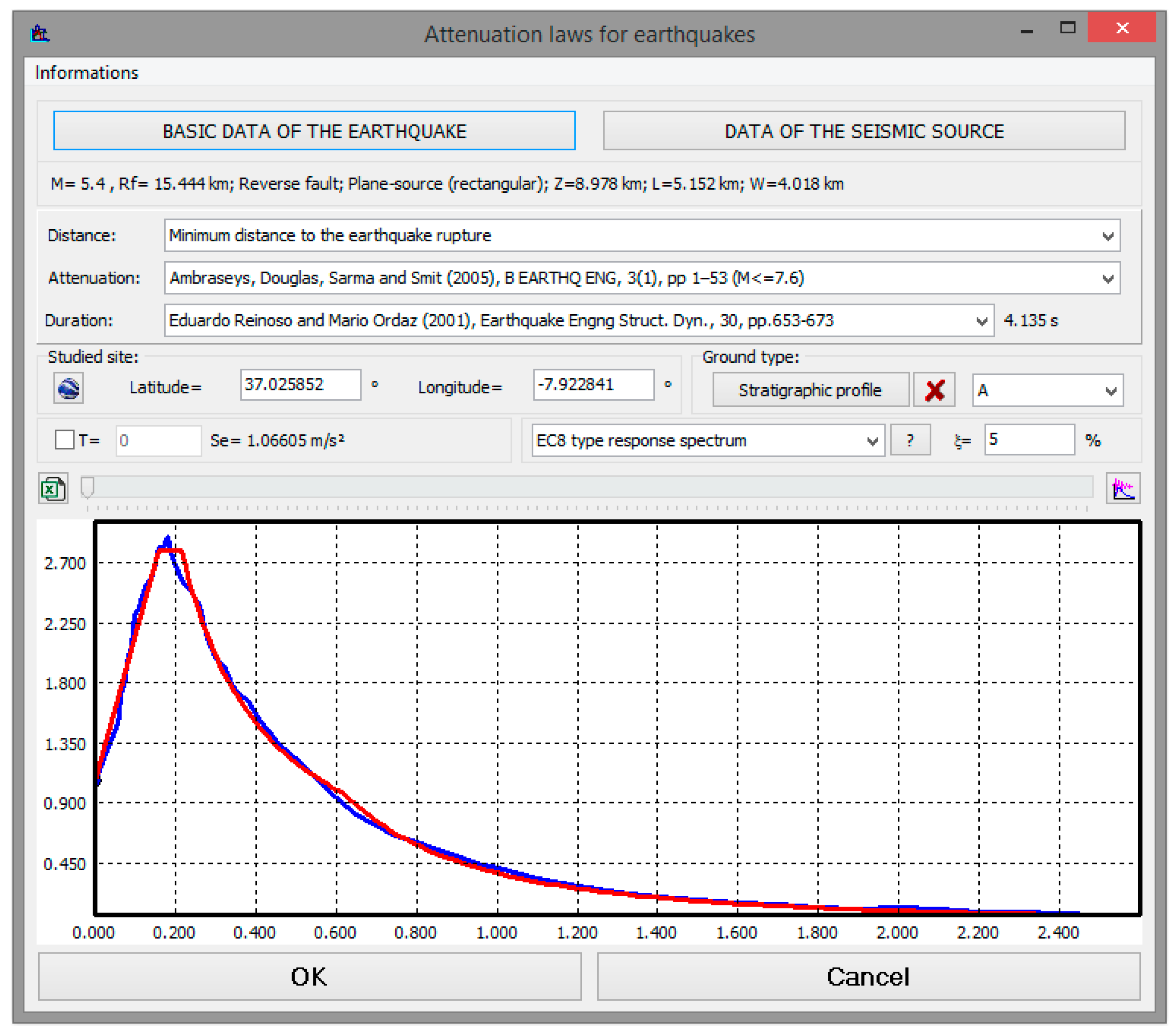
In Figure 5, an example of an EC8-like response spectrum adjusted to the results of a GMPE is presented.
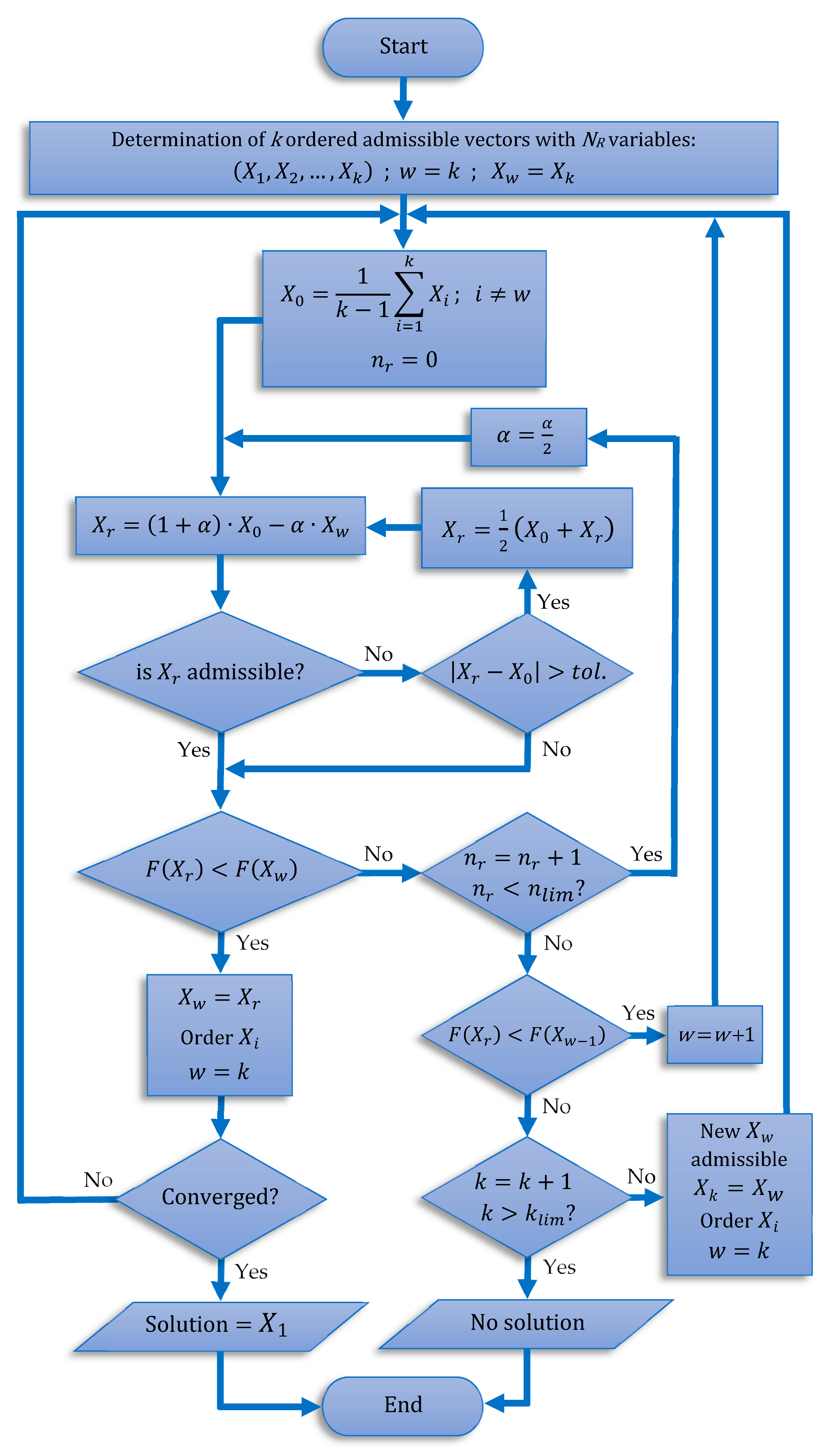
In the implemented approach, the optimization problem is solved by using a variation of the complex method [47,48] (Figure 6), which seems to work properly to obtain the solution, just by looking to Figure 5. However, some care was taken in the parameter definition and in the determination of the initial admissible solutions to obtain better results. The values of the parameters presented in Figure 6 that were adopted as default are k = 16, α = 1.3, nlim = 7 and klim = 18, which were obtained by a trial and error process in order to achieve a compromise between speed and accuracy. For the initial admissible solutions, the vectors are randomly selected so that TB is always lower than the period corresponding to the maximum spectral acceleration, and TC is always higher.
Many pairs of magnitude and distance were used to test the implemented optimization procedure. Results seem to indicate that good fitting was possible to obtain (see the example of Figure 5). It was also interesting to notice that the obtained αa values were different than 2.5 in most cases ( in the example presented in Figure 5), which is the value adopted in the response spectrum of Part 1 of Eurocode 8 (EC8-1).
4. Capacity Curves
In the proposed approach, the vulnerability assessment is based on capacity curves that are computed as described in the EC8 and which are used for NSA. A capacity curve is the nonlinear relation between the displacement of the control node (dn), which is normally the centre of mass of the roof of the building, and the base shear force (Fb).
The first step of any NSA method consists in the idealization of a single degree of freedom (SDOF), with stiffness k* and mass m* (Figure 7), which is equivalent to the initial multiple degrees of freedom (MDOF) dynamic system.
The transformation process of the initial dynamic system with N degrees of freedom (DOF) is done throughout the adoption of a transformation factor (Γ) given by:
with mi being the mass associated to each DOF in the MDOF dynamic system, and ϕi being the configuration of the deformed shape that is adopted in the transformation process (normalized such as ϕn = 1 in the control node n).
Next, it is necessary to obtain the capacity curve of the MDOF system (Figure 7d), which can be computed by using any structural analysis software with that option. To do so, a set of forces (F0i) are applied to the structure in each DOF. It is advisable to normalise these forces, so that the sum equals the unity (), that being:
In consequence, the base shear force will be equal to the load parameter (λ) that is normally computed by the pushover analysis software:
The EC8 indicates that two force patterns must be considered to compute the capacity curves, which are a function of the adopted deformed shape configuration:
- A uniform pattern, proportional to the mass of each degree of freedom, that being ϕn = 1 (Figure 7a);
- a modal-like pattern, which can be proportional to the distance between the base (Figure 7b) and the degree of freedom (DOF), the configuration of the simplified Rayleigh method or corresponding to the configuration of a given computed vibration mode, normally the one with the highest mass participation in the direction where the forces are applied (Figure 7c).
These forces can be obtained automatically by using the developed computer object, and instantly exported to MS Excel, to be then introduced in any structural nonlinear analysis software.
According to the EC8, the two lateral vertical load patterns must be applied in both the positive and negative plan directions of the building (X and Y), and an accidental eccentricity of the centre of mass must also be considered (three mass centres for each direction). Accounting for all these rules, it is necessary to consider at least 24 capacity curves (2 × 2 × 2 × 3 = 24) for each building.
After obtaining the capacity curves of the MDOF structural system, it is possible to compute the capacity curves for the equivalent SDOF system (Figure 7e) just by using the transformation factor:
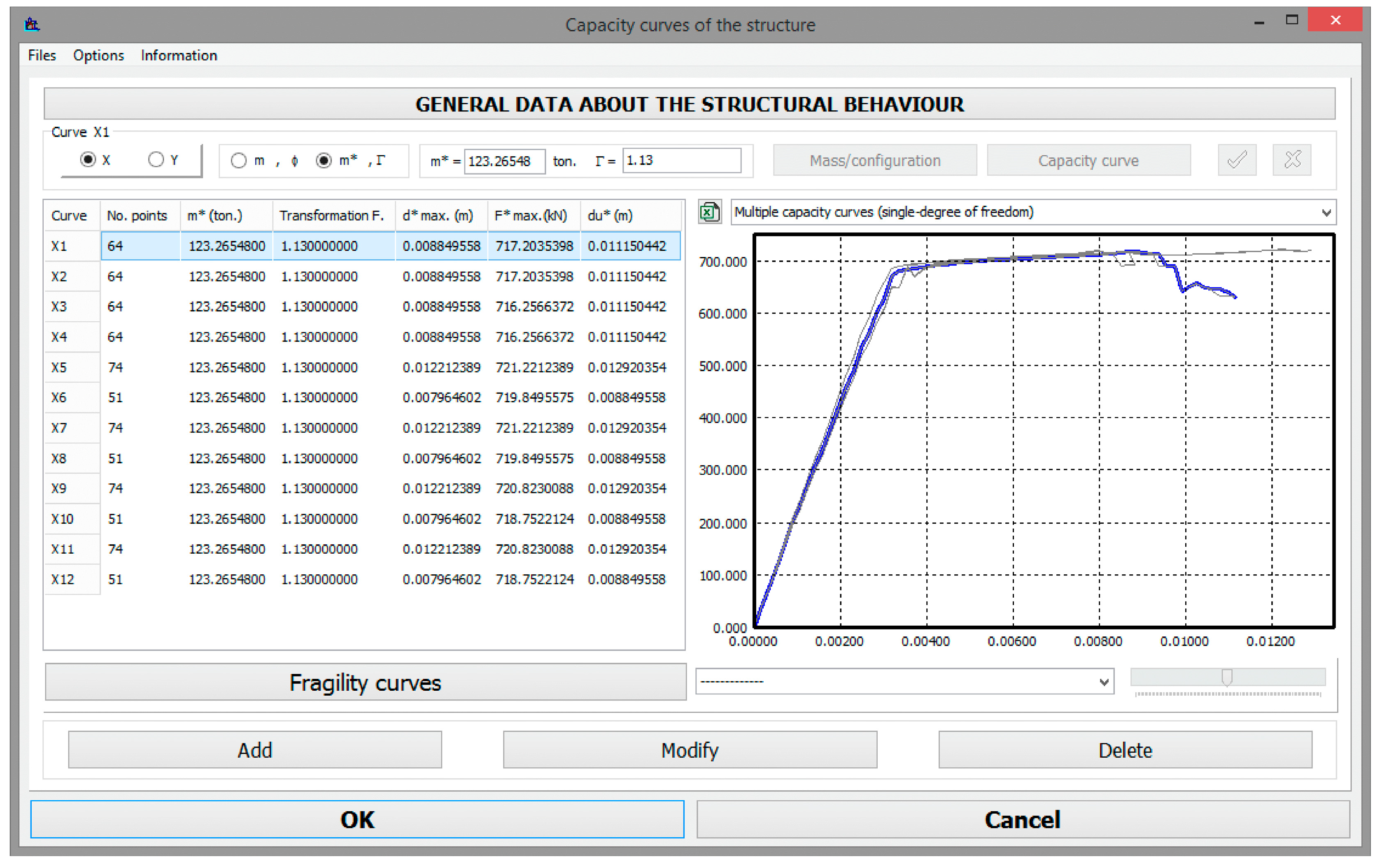
In Figure 8, the user interface of the developed capacity curve computer object is presented, showing 12 capacity curves for the X direction as an example. This interface allows to import the results of a given nonlinear structural analysis software, throughout the reading of a text file with the capacity curve values.
5. Damage Assessment
The damage assessment computer object is the most complex one. This object has multiple constructors because the algorithms that are used to evaluate the damage depend on the type of seismic action that is used to create the object (Figure 9).
Damage is evaluated based on the performance point (the EC8 target displacement) and considering the limit states (LS) that are currently presented in Part 3 of Eurocode 8 (EC8-3), which are the LS of damage limitation (DL), the LS of significant damage (SD) and the LS of near collapse (NC), and also considering the LS for operationality (OP), as it is already presented in the Italian code NTC2018 [49,50], and as it will probably be in the future generation of the Eurocodes [51], as presented in Figure 10 (where du is the ultimate displacement). The performance point may be computed using different NSA methods, namely the CSM and the N2 method, which are the ones that are implemented in the present version of the developed software.
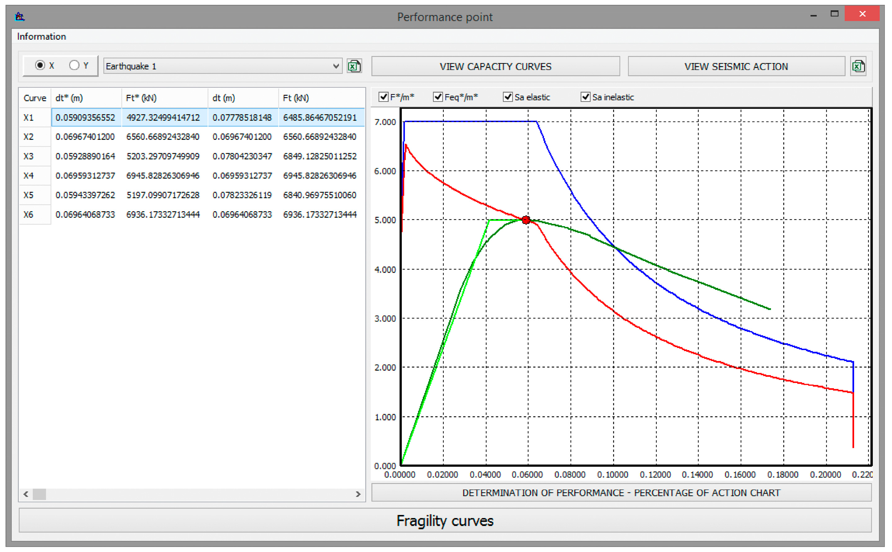
The main difficulty dealing with the determination of the damage level related to the LS presented in the EC8-3 is that each capacity curve presents different LS displacement values. This means that a capacity curve with higher resistance may also present a higher damage level, or even collapse, if it exhibits much less ductility. So, it is not very evident which is the capacity curve that presents the worst results in terms of damage, namely in accordance with the EC8-3. To overcome this problem, a new concept is proposed: The performance curve (Figure 11).
The performance curve represents the relation between a displacement of the control node and the percentage of a given response spectrum (used as input), which is necessary to obtain a target displacement (performance point) corresponding to the predefined displacement level. Basically, it represents all the performance points that are obtained when different percentages of a given response spectrum are considered. In this way, it becomes quite evident which capacity curves are the most problematic ones for a given damage LS, as can observed in Figure 11.
At a first glance, this proposal seems to be quite inefficient, computationally speaking, because the analysis should be carried out many times for each percentage of the seismic action, which might be very time consuming, particularly when adopting iterative procedures. However, this is not the case for the implemented approach because the procedures of both the CSM and N2 methods are inverted. Instead of obtaining a target displacement (the performance point) associated to a given spectral acceleration, as usual, in the proposed approach the percentage of the spectral acceleration associated to a given predefined displacement is computed. This process is described in detail in the following sections.
5.1. N2 Method
The N2 is the NSA method that is presented in the Annex B of the EC8-1, with two possible approaches: An iterative and a non-iterative approach. Both approaches were implemented in the developed seismic assessment software, and the proposed algorithms are described in detail in Appendix A.
As presented in the EC8, first it is necessary to obtain a elastic-perfectly plastic relation between forces (F*) and displacements (d*) in the SDOF dynamic system, ensuring that the strain energy deformation of the equivalent system is the same as for the initial system (Figure 12).
For a given target displacement , it is possible to obtain the following equations:
The period (T*) of the idealized nonlinear system will be equal to:
To obtain the percentage of the spectral acceleration (%Se) of an EC8-like response spectrum, corresponding to the displacement associated to a given LS, the following equations must be computed:
- If T* ≥ TC (the medium and long period range), then:
- If T* < TC (the short period range), then:
and if Fy*/m* > Sa*, then Sa* = Sea* (see Equation (16)).
With this approach, the performance curve can be obtained and the worst capacity curve for a given LS can be determined very quickly, as can be seen in the video presented in the Supplementary Materials.
5.2. Capacity Spectrum Method (CSM)
CSM is a method proposed in the ATC-40 and is implemented in a lot of software developed around the world for seismic assessment, like HAZUS, for example, sometimes with some variations, such as in the case of the approach that is proposed in the technical notes of the new Italian code NTC2018. The iterative approach of the CSM is not as simple and fast as the N2 method. However, with the proposed approach, it becomes much simpler, as presented in Figure 13, and considering:
is obtained throughout Equations (4) and (5), and the equivalent damping (in percentage) can be computed as proposed in the ATC-40 and in the technical notes of the NTC2018, as:
where is a factor that accounts for the real hysteresis loops, and which is dependent on the type of the material, structural details and earthquake duration. All the three types of energy dissipation behaviour (CSM-A, CSM-B and CSM-C) presented in ATC-40 were implemented in the developed software.
The implemented iterative procedure used to compute the performance point based on the CSM is presented in Appendix B.
5.3. Fragility Curves
In the context of modern seismic assessment, it is common to adopt probabilistic approaches for damage evaluation, where the probability of exceeding a given damage LS (D) corresponds to the following equation:
where is the probability density function of the ground motion A, normally determined throughout a probabilistic seismic hazard analysis (already considering the local site effects), and is the structural fragility, which can be defined as the probability of the damage level Di exceeding a given LS (), for a given ground motion level ().
The use of fragility curves has become popular since the development of the HAZUS software, and can be computed for each performance point (the target displacement dt) as follows:
with Φ being the cumulative distribution function for the normal distribution, being the mean value of the displacement corresponding to a given damage LS (Di) and being the standard deviation of the natural logarithm of the displacement .
The probability of achieving a given damage LS Di (OP = D1, DL = D2, SD = D3, NC = D4 and D5 = collapse) is given by:
The fragility curves, which are the relations between any displacement and any , are also computed by the developed software. The values can be introduced by the user in an interface developed for that purpose.
6. Output Results
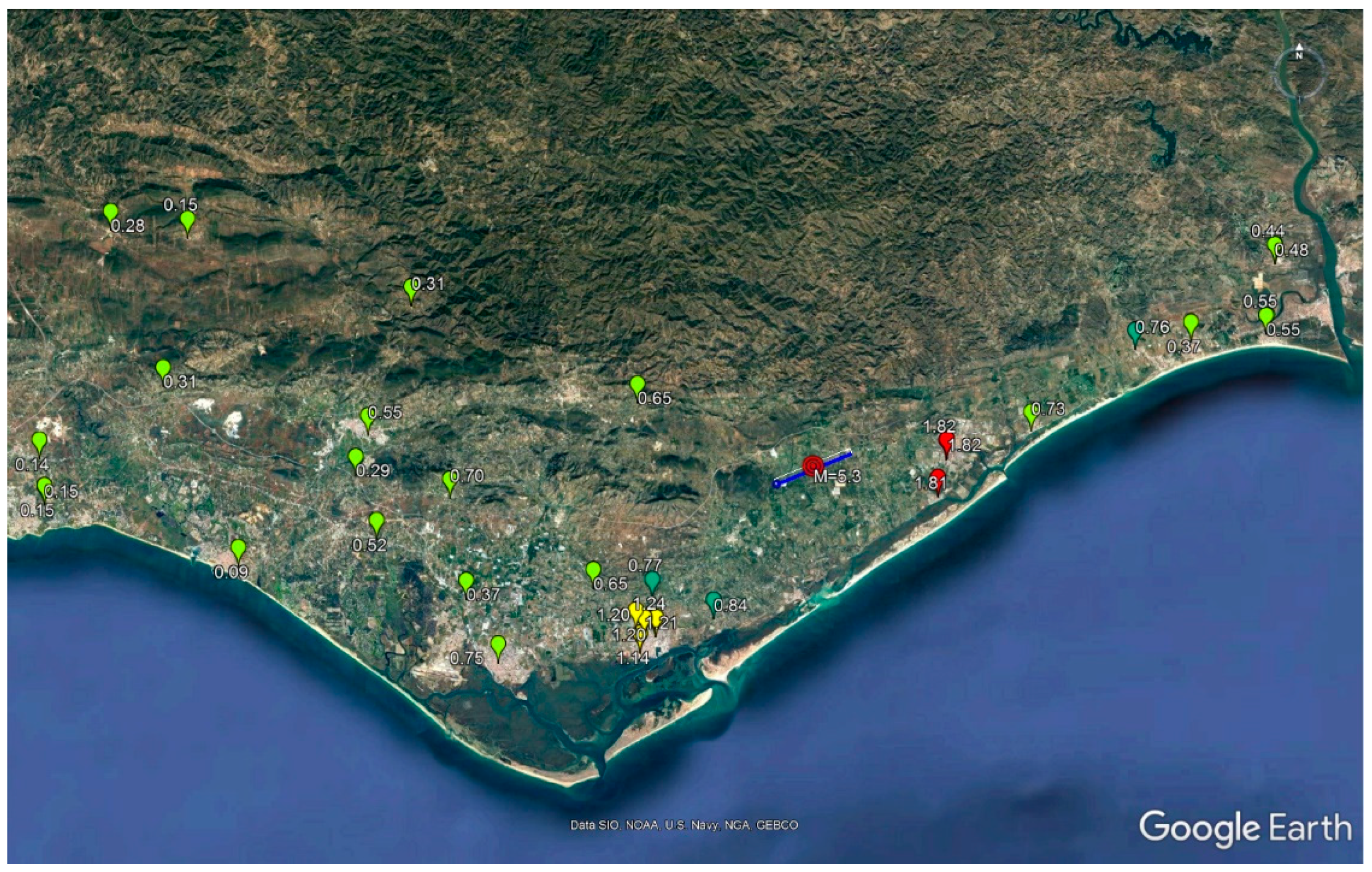
The seismic assessment output results can be presented as a ranked list in the software interface, or can be automatically exported to external software, such as to MS Excel (through the Windows Clipboard) or to Google Earth (through a kml file, as presented in Figure 14).
In PERSISTAH software, results can be filtered by country, region, municipality, building typology or soil type, among other options. To rank the seismic risk of each building, the following score is adopted (the score level is proportional to the seismic risk):
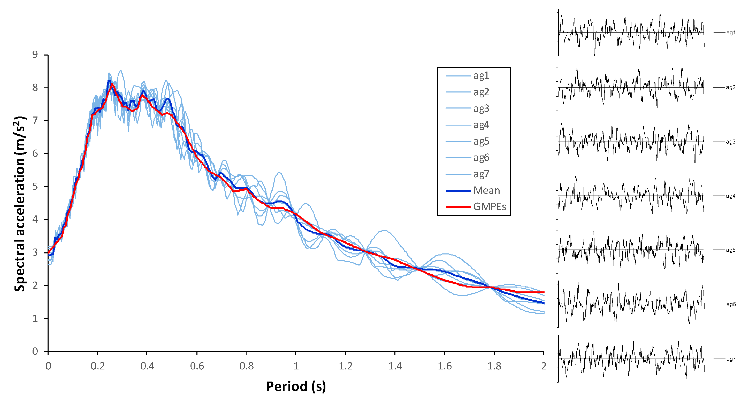
In order to demonstrate the accuracy of the proposed approach, the results obtained with the developed software were compared against the results obtained with a more accurate time-history nonlinear dynamic analysis of a structure (Figure 15) that was analysed in a previous study [52]. A point source (inverse fault) magnitude M = 6.5 earthquake scenario was considered, with an epicentral distance equal to D = 13.972 km. The response spectrum was computed for a soft soil site using one of the already implemented GMPEs [53]. Using the proposed optimization process, an EC8-like response spectrum was adjusted to the GMPEs (Figure 16), obtaining αa = 2.52, TB = 0.230 s, TC = 0.496 s and TD = 1.771 s. Then, seven artificial accelerograms were generated, as proposed in the EC8, so that the mean response spectrum matched the response spectrum obtained with the GMPEs (Figure 17). The ground motion duration was computed using the empirical expression proposed by Reinoso and Ordaz [54]. The results obtained with the different methods are presented in Table 2 and show good agreement between the results obtained with the proposed algorithms and the more accurate NDA results.
More examples of the output interfaces of the developed software are presented in Appendix A and Appendix B.
7. Conclusions
A new integrated system for the seismic assessment of individual buildings is presented. The developed software produces results very quickly and allows an easy comparison between the behaviour of different buildings, in different countries and regions, and between any given earthquake scenario or a code-based seismic action. More than simply presenting a new computational strategy for the development of seismic assessment tools based on puzzle-like independent computer objects, two new approaches are also proposed: (1) The use of an optimization process to adjust an EC8-like response spectrum to the results of an attenuation law in an earthquake scenario option; (2) the proposal of two algorithms (for the CSM and N2 methods) for computing a relation between the structural displacements and the percentage of a seismic action, which was designated by performance curve.
The results that were obtained with the adjusted response spectrum (computed with the proposed optimization process) may present a different ratio between the maximum spectral acceleration and the PGA when compared with the EC8 response spectrum, which uses a constant value of 2.5. Results show that the developed algorithms exhibit good precision when compared with the results obtained with time-history nonlinear dynamic analysis. The obtained results also show that the proposed performance curves allow better comparison between the results obtained with different capacity curves and analysis methods.
Supplementary Materials
The following are available online at https://www.mdpi.com/2076-3417/9/23/5088/s1. Video S1_PERSISTAH: Short video that shows some of the capabilities of the developed seismic risk assessment tool.
Funding
This research was funded by INTERREG-POCTEP España-Portugal program and the European Regional Development Fund, grant number 0313_PERSISTAH_5_P.
Conflicts of Interest
The author declares no conflict of interest. The funders had no role in the design of the study; in the collection, analyses or interpretation of data; in the writing of the manuscript; or in the decision to publish the results.
Appendix A
In this appendix, the algorithm for the iterative approach of the N2 method that was implemented in the developed software is described.
If it is considered unlimited elastic behaviour, then the structural performance may be determined based on the spectral acceleration for the period T*, that is:
where is the elastic acceleration response spectrum at period T*.
Main steps of the algorithm (Figure A1):
- The area (Em*) under the capacity curve corresponding to the limit point (the maximum force of the capacity curve, which is the pair dm*, Fm*) is determined using Equation (13) with .The initial stiffness of the idealized elastic-perfectly plastic structural system will be equal toInstead of computing through Equation (A2) in the developed computer routines it is also possible to obtain this stiffness for a given percentage of the force , as presented in the technical instructions of the NTC2018.Figure A1. Flowchart of the developed algorithm for the iterative N2 method.
![Applsci 09 05088 g0a1]()
- The performance point (the target displacement dti*) of the SDOF system is computed as follows:
- If T* < TC then:
- If T* ≥ TC then dti* = det*:
- The difference ∆dti* between the old performance point and the new performance point is determined. If ∆dti* is higher than a given maximum error, then the area (Eti*) under the capacity curve corresponding to the new target displacement dti* is computed.
- If dti* < dm* then:
- The procedure returns to step 2 until convergence is reached.

Finally, when the convergence criterium is achieved, the target displacement dt (the performance point of the MDOF structural system) is obtained in accordance with the following expression:
An example of the output interface for the N2 method is presented in Figure A2.
It is also possible to use the non-iterative approach of the N2 method, which is a little bit faster. For that option, only Equations (A6) and (A7), or (A8) and (A9) are used, depending if du* > dm* or not, and considering the ultimate displacement in place of .
The maximum number of iterations is also selectable by the user.
When comparing the results for the iterative and for the non-iterative approaches of the N2 method, it was possible to observe that the results obtained with the iterative approach are more conservative, so that probably is a better approach for seismic assessment of individual buildings.
Figure A2.
Example of the output interface for the N2 method.

Appendix B
This appendix presents the algorithm that was developed for the CSM, which is implemented in the developed seismic assessment tool.
In theory, both the CSM and N2 methods should present very close results. In fact, when comparing Figure A2 and Figure A3, it becomes evident that the results obtained with the implemented CSM and N2 methods are quite similar when using the same capacity curves and response spectra, but only if adopting , which is the value corresponding to a low dissipative system in the ATC-40 (CSM-C).
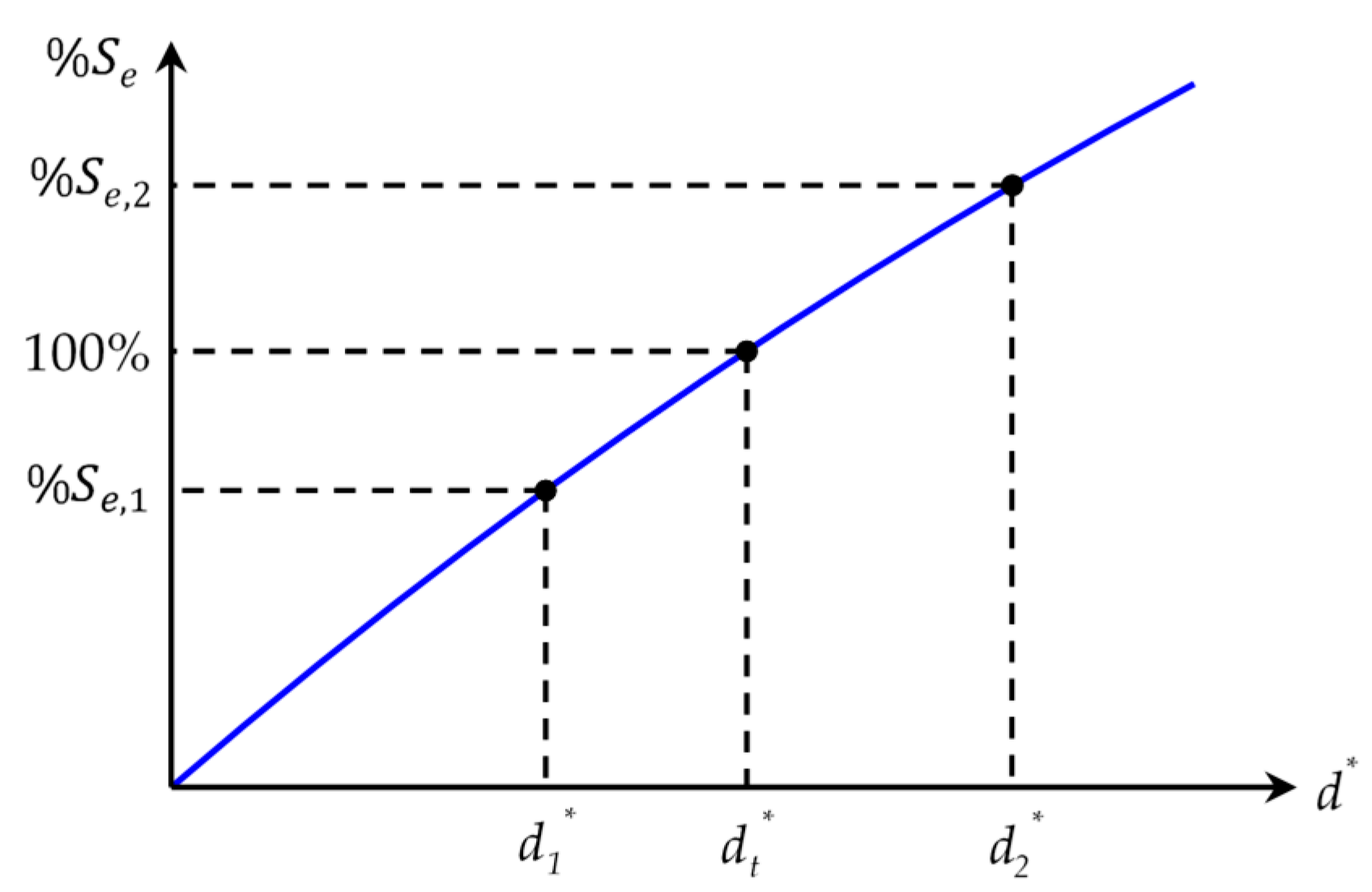
The developed algorithm uses the concept of a performance curve (Equation (18)) to compute the performance point (the target displacement), and involves the following main steps:
- At first, the limit points of the intervals () and () of the performance curve where the target point () is located (Figure A4) are computed by scanning the points of the performance curve.
- Then, a simple iterative process is adopted, until the convergence is reached with the desired error precision:
- If then , otherwise .
- The iterative process is repeated until and is almost exactly 100%.
This iterative process is quite fast and simple, namely when comparing with the proposed approaches in the ATC-40.
Figure A3.
Example of the output interface for the capacity spectrum method (CSM).

Figure A4.
Iterative process adopted for the CSM.

References
- Augenti, N.; Cosenza, E.; Dolce, M.; Manfredi, G.; Masi, A.; Samela, L. Performance of School Buildings during the 2002 Molise, Italy, Earthquake. Earthq. Spectra 2004, 20, S257–S270. [Google Scholar] [CrossRef]
- Puglia, R.; Vona, M.; Klin, P.; Ladina, C.; Masi, A.; Priolo, E.; Silvestri, F. Analysis of Site Response and Building Damage Distribution Induced by the 31 October 2002 Earthquake at San Giuliano di Puglia (Italy). Earthq. Spectra 2013, 29, 497–526. [Google Scholar] [CrossRef]
- Di Ludovico, M.; Digrisolo, A.; Moroni, C.; Graziotti, F.; Manfredi, V.; Prota, A.; Dolce, M.; Manfredi, G. Remarks on damage and response of school buildings after the Central Italy earthquake sequence. Bull. Earthq. Eng. 2018, 10, 5679–5700. [Google Scholar] [CrossRef]
- Estêvão, J.M.C.; Ferreira, M.A.; Morales-Esteban, A.; Martínez-Álvarez, F.; Fazendeiro-Sá, L.; Requena-García-Cruz, V.; Segovia-Verjel, M.L.; Oliveira, C.S. Earthquake resilient schools in Algarve (Portugal) and Huelva (Spain). In Proceedings of the 16th European Conference on Earthquake Engineering (16ECEE), Thessaloniki, Greece, 18–21 June 2018; pp. 1–11. [Google Scholar]
- Chrysostomou, C.Z.; Kyriakides, N.; Papanikolaou, V.K.; Kappos, A.J.; Dimitrakopoulos, E.G.; Giouvanidis, A.I. Vulnerability assessment and feasibility analysis of seismic strengthening of school buildings. Bull. Earthq. Eng. 2015, 13, 3809–3840. [Google Scholar] [CrossRef]
- Xu, Z.; Lu, X.; Zeng, X.; Xu, Y.; Li, Y. Seismic loss assessment for buildings with various-LOD BIM data. Adv. Eng. Inform. 2019, 39, 112–126. [Google Scholar] [CrossRef]
- Clementi, F.; Quagliarini, E.; Maracchini, G.; Lenci, S. Post-World War II Italian school buildings: Typical and specific seismic vulnerabilities. J. Build. Eng. 2015, 4, 152–166. [Google Scholar] [CrossRef]
- Ventura, C.E.; Bebamzadeh, A.; Fairhurst, M.; Turek, M.; Taylor, G.; Finn, W.D.L. Performance-based seismic retrofit of school buildings in British Columbia, Canada–an overview. In Proceedings of the 16th World Conference on Earthquake Engineering (16WCEE), Santiago, Chile, 9–13 January 2017; pp. 1–12. [Google Scholar]
- El-Betar, S.A. Seismic vulnerability evaluation of existing R.C. buildings. HBRC J. 2018, 14, 189–197. [Google Scholar] [CrossRef]
- Korkmaz, M.; Ozdemir, M.A.; Kavali, E.; Cakir, F. Performance-based assessment of multi-story unreinforced masonry buildings: The case of historical Khatib School in Erzurum, Turkey. Eng. Fail. Anal. 2018, 94, 195–213. [Google Scholar] [CrossRef]
- O’Reilly, G.J.; Perrone, D.; Fox, M.; Monteiro, R.; Filiatrault, A. Seismic assessment and loss estimation of existing school buildings in Italy. Eng. Struct. 2018, 168, 142–162. [Google Scholar] [CrossRef]
- Oyguc, R. Seismic performance of RC school buildings after 2011 Van earthquakes. Bull. Earthq. Eng. 2016, 14, 821–847. [Google Scholar] [CrossRef]
- Freeman, S.A. Review of the development of the capacity spectrum method. ISET J. Earthq. Technol. 2004, 41, 1–13. [Google Scholar]
- ATC. Seismic Evaluation and Retrofit of Concrete Buildings, Volume 1; Applied Technology Council: Redwood City, CA, USA, 1996; p. 341. [Google Scholar]
- Fajfar, P. Analysis in seismic provisions for buildings: Past, present and future. Bull. Earthq. Eng. 2018, 16, 2567–2608. [Google Scholar] [CrossRef]
- Fajfar, P. A nonlinear analysis method for performance-based seismic design. Earthq. Spectra 2000, 16, 573–592. [Google Scholar] [CrossRef]
- CEN. Eurocode 8, Design of Structures for Earthquake Resistance-Part 1: General Rules, Seismic Actions and Rules for Buildings. EN 1998-1:2004; Comité Européen de Normalisation: Brussels, Belgium, 2004; p. 229. [Google Scholar]
- Andredakis, I.; Proietti, C.; Fonio, C.; Annunziato, A. Seismic Risk Assessment Tools-Workshop; JRC Technical Reports; European Union: Brussels, Belgium, 2017; p. 37. [Google Scholar] [CrossRef]
- Crowley, H.; Colombi, M.; Crempien, J.; Erduran, E.; Lopez, M.; Liu, H.; Mayfield, M.; Milanesi, M. GEM1 Seismic Risk Report: Part 1, GEM Technical Report 2010-5; GEM Foundation: Pavia, Italy, 2010. [Google Scholar]
- GFDRR. Understanding Risk-Review of Open Source and Open Access Software Packages Available to Quantify Risk From Natural Hazards; International Bank for Reconstruction and Development/International Development Association or The World Bank: Washington, DC, USA, 2014; p. 67. [Google Scholar]
- Lyle, T.S.; Hund, S.V. Way Forward for Risk Assessment Tools in Canada; Open File 8255; Geological Survey of Canada: Vancouver, BC, Canada, 2017. [CrossRef]
- Nurlu, M.; Fahjan, Y.; Eravci, B.; Baykal, M.; Yenilmez, G.; Yalçin, D.; Yanik, K.; Kara, F.İ.; Pakdamar, F. Rapid estimation of earthquake losses in Turkey using AFAD-RED system. In Proceedings of the Second European Conference on Earthquake Engineering, Istanbul, Turkey, 25–29 August 2014; pp. 1–8. [Google Scholar]
- Sedan, O.; Negulescu, C.; Terrier, M.; Roulle, A.; Winter, T.; Bertil, D. Armagedom—A Tool for Seismic Risk Assessment Illustrated with Applications. J. Earthq. Eng. 2013, 17, 253–281. [Google Scholar] [CrossRef]
- Aguilar-Meléndez, A.; Ordaz Schroeder, M.G.; De la Puente, J.; González Rocha, S.N.; Rodriguez Lozoya, H.E.; Córdova Ceballos, A.; García Elías, A.; Calderón Ramón, C.M.; Escalante Martínez, J.E.; Laguna Camacho, J.R.; et al. Development and Validation of Software CRISIS to Perform Probabilistic Seismic Hazard Assessment with Emphasis on the Recent CRISIS2015. Computación y Sistemas 2017, 21. [Google Scholar] [CrossRef]
- Cardona, O.D.; Ordaz, M.G.; Reinoso, E.; Yamín, L.E.; Barbat, A.H. CAPRA-Comprehensive Approach to Probabilistic Risk Assessment: International Initiative for Risk Management Effectiveness. In Proceedings of the 15th World Conference on Earthquake Engineering, Lisbon, Portugal, 24–28 September 2012; pp. 1–10. [Google Scholar]
- Müller, M.; Vorogushyn, S.; Maier, P.; Thieken, A.H.; Petrow, T.; Kron, A.; Büchele, B.; Wächter, J. CEDIM Risk Explorer—A map server solution in the project “Risk Map Germany”. Nat. Hazards Earth Syst. Sci. 2006, 6, 711–720. [Google Scholar] [CrossRef]
- Abo El Ezz, A.; Smirnoff, A.; Nastev, M.; Nollet, M.-J.; McGrath, H. ER2-Earthquake: Interactive web-application for urban seismic risk assessment. Int. J. Disaster Risk Reduct. 2019, 34, 326–336. [Google Scholar] [CrossRef]
- Hancilar, U.; Tuzun, C.; Yenidogan, C.; Erdik, M. ELER software–a new tool for urban earthquake loss assessment. Nat. Hazards Earth Syst. Sci. 2010, 10, 2677–2696. [Google Scholar] [CrossRef]
- Eguchi, R.T.; Goltz, J.D.; Seligson, H.A.; Flores, P.J.; Blais, N.C.; Heaton, T.H.; Bortugno, E. Real-Time Loss Estimation as an Emergency Response Decision Support System: The Early Post-Earthquake Damage Assessment Tool (EPEDAT). Earthq. Spectra 1997, 13, 815–832. [Google Scholar] [CrossRef]
- Robinson, D.; Fulford, G.; Dhu, T. EQRM: Geoscience Australia’s Earthquake Risk Model. Technical Manual Version 3.0; Geoscience Australia Record 2005/01; Australian Government: Canberra, Australia, 2005.
- FEMA. Hazus®-MH 2.1-Advanced Engineering Building Module (AEBM). Technical and User’s Manual; Federal Emergency Management Agency (FEMA): Washington, DC, USA, 2002.
- Pranantyo, I.R.; Fadmastuti, M.; Chandra, F. InaSAFE applications in disaster preparedness. AIP Conf. Proc. 2015, 1658, 060001. [Google Scholar] [CrossRef]
- Erdik, M.; Aydinoglu, N.; Fahjan, Y.; Sesetyan, K.; Demircioglu, M.; Siyahi, B.; Durukal, E.; Ozbey, C.; Biro, Y.; Akman, H.; et al. Earthquake risk assessment for Istanbul metropolitan area. Earthq. Eng. Eng. Vib. 2003, 2, 1–23. [Google Scholar] [CrossRef]
- Sousa, M.L.; Costa, A.C.; Carvalho, A.; Coelho, E. An automatic seismic scenario loss methodology integrated on a geographic information system. In Proceedings of the 13th World Conference on Earthquake Engineering, Vancouver, BC, Canada, 1–6 August 2004; pp. 1–13. [Google Scholar]
- Elnashai, A.; Hampton, S.; Lee, J.S.; McLaren, T.; Myers, J.D.; Navarro, C.; Spencer, B.; Tolbert, N. Architectural Overview of MAEviz–HAZTURK. J. Earthq. Eng. 2008, 12, 92–99. [Google Scholar] [CrossRef]
- Muto, M.; Krishnan, S.; Beck, J.L.; Mitrani-Reiser, J. Seismic loss estimation based on end-to-end simulation. In Proceedings of the International Symposium on Life-Cycle Civil Engineering, IALCCE’08, Varenna, Lake Como, Italy, 10–14 June 2008; pp. 1–6. [Google Scholar]
- Silva, V.; Crowley, H.; Pagani, M.; Monelli, D.; Pinho, R. Development of the OpenQuake engine, the Global Earthquake Model’s open-source software for seismic risk assessment. Nat. Hazards 2014, 72, 1409–1427. [Google Scholar] [CrossRef]
- Rosset, P.; Bishop, B.; Tolis, S.; Wyss, M. QLARM: A Global Model for Earthquake Loss Estimates in Real-Time and Scenario Modes. In Proceedings of the UNISDR Science and Technology Conference on the implementation of the Sendai Framework for Disaster Risk Reduction 2015–2030, Geneva, Switzerland, 27–29 January 2016. [Google Scholar]
- Mota de Sá, F.; Ferreira, M.A.; Oliveira, C.S. QuakeIST® earthquake scenario simulator using interdependencies. Bull. Earthq. Eng. 2016, 14, 2047–2067. [Google Scholar] [CrossRef]
- Bell, R.G.; Reese, S.; King, A.B. Regional RiskScape: A multi-hazard loss modelling tool. In Proceedings of the Coastal Communities Natural Disasters, Auckland, New Zealand; pp. 1–4.
- Anagnostopoulos, S.; Providakis, C.; Salvaneschi, P.; Athanasopoulos, G.; Bonacina, G. SEISMOCARE: An efficient GIS tool for scenario-type investigations of seismic risk of existing cities. Soil Dyn. Earthq. Eng. 2008, 28, 73–84. [Google Scholar] [CrossRef]
- Molina, S.; Lang, D.H.; Lindholm, C.D. SELENA–An open-source tool for seismic risk and loss assessment using a logic tree computation procedure. Comput. Geosci. 2010, 36, 257–269. [Google Scholar] [CrossRef]
- Latcharote, P.; Terada, K.; Hori, M.; Imamura, F. A Prototype Seismic Loss Assessment Tool Using Integrated Earthquake Simulation. Int. J. Disaster Risk Reduct. 2018, 31, 1354–1365. [Google Scholar] [CrossRef]
- Estêvão, J.M.C.; Carvalho, A. The role of source and site effects on structural failures due to Azores earthquakes. Eng. Fail. Anal. 2015, 56, 429–440. [Google Scholar] [CrossRef]
- Estêvão, J.M.C.; Oliveira, C.S. Point and fault rupture stochastic methods for generating simulated accelerograms considering soil effects for structural analysis. Soil Dyn. Earthq. Eng. 2012, 43, 329–341. [Google Scholar] [CrossRef]
- Estêvão, J.M.C. Utilização do programa EC8spec na avaliação e reforço sísmico de edifícios do Algarve. In Proceedings of the 10° Congresso Nacional de Sismologia e Engenharia Sísmica, Ponta Delgada, Açores, Portugal; pp. 1–11. CD25(In Portuguese).
- Hu, S.-y.; Cheng, J.-H. Development of the unlocking mechanisms for the complex method. Comput. Struct. 2005, 83, 1991–2002. [Google Scholar] [CrossRef]
- Rao, S.S. Engineering optimization; John Wiley & sons, Inc.: New York, NY, USA, 1996; p. 922. [Google Scholar]
- NTC. Aggiornamento delle «Norme tecniche per le costruzioni»; Ministero delle infrastrutture e dei trasporti: Roma, Italy, 2018. (In Italian)
- NTC. Istruzioni per l’applicazione dell’«Aggiornamento delle “Norme tecniche per le costruzioni”» di cui al decreto ministeriale 17 gennaio 2018; Ministero delle infrastrutture e dei trasporti: Roma, Italy, 2019. (In Italian)
- Bisch, P. Eurocode 8. Evolution or Revolution? In Recent Advances in Earthquake Engineering in Europe: 16th European Conference on Earthquake Engineering-Thessaloniki 2018; Pitilakis, K., Ed.; Springer International Publishing: Cham, Switzerland, 2018; pp. 639–660. [Google Scholar] [CrossRef]
- Estêvão, J.M.C. Feasibility of using neural networks to obtain simplified capacity curves for seismic assessment. Buildings 2018, 8, 151. [Google Scholar] [CrossRef] [Green Version]
- Ambraseys, N.N.; Douglas, J.; Sarma, S.K.; Smit, P.M. Equations for the Estimation of Strong Ground Motions from Shallow Crustal Earthquakes Using Data from Europe and the Middle East: Horizontal Peak Ground Acceleration and Spectral Acceleration. Bull. Earthq. Eng. 2005, 3, 1–53. [Google Scholar] [CrossRef] [Green Version]
- Reinoso, E.; Ordaz, M. Duration of strong ground motion during Mexican earthquakes in terms of magnitude, distance to the rupture area and dominant site period. Earthq. Eng. Struct. Dyn. 2001, 30, 653–673. [Google Scholar] [CrossRef]
Figure 1.
Global scheme for the existing seismic risk assessment tools.

Figure 2.
Puzzle-like interconnection of the developed computer objects.

Figure 3.
Input/output Eurocode 8 (EC8)-type response spectrum user interface.

Figure 4.
Types of possible sources and distances to the earthquake: (a) Point source; (b) line source; (c) fault plane (rectangular).
Figure 4.
Types of possible sources and distances to the earthquake: (a) Point source; (b) line source; (c) fault plane (rectangular).

Figure 5.
Input/output ground-motion prediction equations (GMPEs) user interface with an EC8-like adjusted response spectrum.
Figure 5.
Input/output ground-motion prediction equations (GMPEs) user interface with an EC8-like adjusted response spectrum.

Figure 6.
Flowchart of the implemented complex method algorithm.

Figure 7.
Scheme for obtaining the buildings capacity curves. Force patterns: (a) Uniform; (b) proportional to the high of the building; (c) based on a given mode of vibration. (d) Capacity curve of the multiple degrees of freedom (MDOF) dynamic system. (e) Capacity curve of the equivalent single degree of freedom (SDOF) dynamic system.

Figure 8.
Input/output capacity curve computer object user interface.

Figure 9.
Connections between the damage assessment computer object that computes the performance point and the other independent objects.
Figure 9.
Connections between the damage assessment computer object that computes the performance point and the other independent objects.

Figure 10.
Example of the localization of the limit states (LS) in one capacity curve.

Figure 11.
Example of the interface that presents the performance curves.

Figure 12.
Capacity curve of the equivalent perfectly elastic plastic SDOF dynamic system.

Figure 13.
Scheme for obtaining the performance curve, based on the capacity spectrum method (CSM).

Figure 14.
Example of the output that can be automatically exported to Google Earth, with individual building score results, for a given earthquake scenario.
Figure 14.
Example of the output that can be automatically exported to Google Earth, with individual building score results, for a given earthquake scenario.

Figure 15.
Structural system used for the validation of the proposed algorithms.

Figure 16.
Example of the generation of a response spectrum for a given earthquake scenario and an EC8-like response spectrum that is automatically adjusted by the software.
Figure 16.
Example of the generation of a response spectrum for a given earthquake scenario and an EC8-like response spectrum that is automatically adjusted by the software.

Figure 17.
Artificial accelerograms generated for the validation of the developed methodology and the corresponding response spectra.
Figure 17.
Artificial accelerograms generated for the validation of the developed methodology and the corresponding response spectra.


Table 1.
Some of the worldwide developed seismic risk assessment tools.
| SRA Tools | Hazard Module | Vulnerability Module | Exposure Module | GIS Output Results |
|---|---|---|---|---|
| AFAD-RED [22] | ☑ 1 | ☑ | ☑ | ☑ |
| ARMAGEDOM [23] | ☑ 1,2 | ☑ 3,4 | ☑ 6 | ☑ |
| CAPRA+CRISIS [24,25] | ☑ 1,2 | ☑ | ☑ 5,6 | ☑ |
| CEDIM [19,26] | ☑ 1,2 | ☑ 3 | ☑ 5,6 | ☑ |
| ER2-Earthquake [27] | ☑ 1,2 | ☑ 4 | ☑ 6 | ☑ |
| ELER [19,28] | ☑ 1 | ☑ 3,4 | ☑ 6 | ☑ |
| EPEDAT [29] | ☑ 1 | ☑ 3 | ☑ 6 | ☑ |
| EQRM [19,30] | ☑ 1,2 | ☑ | ☑ 5,6 | ☑ |
| HAZUS [31] | ☑ 1,2 | ☑ 4 | ☑ 5,6 | ☑ |
| InaSAFE [32] | ☑ | ☑ | ☑ 5 | ☑ |
| KOERILoss [33] | ☑ 1,2 | ☑ 4 | ☑ 6 | ☑ |
| LNECLoss [19,34] | ☑ 1 | ☑ 3,4 | ☑ 6 | ☑ |
| MAEViz [19,35] | ☑ 1,2 | ☑ | ☑ 5 | ☑ |
| MDLA [36] | ☑ 1,2 | ☑ 4 | ☑ ? | ⊠ |
| OpenQuake [37] | ☑ 1,2 | ☑ 3 | ☑ 6 | ☑ |
| QLARM [38] | ☑ 1 | ☑ | ☑ 6 | ☑ |
| QuakeIST [39] | ☑ 1 | ☑ 3,4 | ☑ 5,6 | ☑ |
| RiskScape [19,40] | ☑ 1 | ☑ 3 | ☑ 5,6 | ☑ |
| SEISMOCARE [41] | ☑ 2 | ☑ 4 | ☑ 5 | ☑ |
| SELENA [42] | ☑ 1,2 | ☑ 4 | ☑ 5,6 | ☑ |
| SLA-IES [43] | ☑ 1 | ☑ 4 | ☑ 5 | ☑ |
1 Deterministic; 2 probabilistic; 3 empirical methods; 4 mechanical methods; 5 individual units; 6 group units.
Table 2.
Displacements obtained with different methods for the structure of the Figure 15.
Table 2.
Displacements obtained with different methods for the structure of the Figure 15.
| Method of Analysis | Displacement at the Top of the Building (m) |
|---|---|
| N2 | 0.05032 |
| CSM-C | 0.04765 |
| CSM-B | 0.03820 |
| CSM-A | 0.03322 |
| DNA minimum | 0.03010 |
| DNA mean | 0.03694 |
| DNA maximum | 0.04519 |
© 2019 by the author. Licensee MDPI, Basel, Switzerland. This article is an open access article distributed under the terms and conditions of the Creative Commons Attribution (CC BY) license (http://creativecommons.org/licenses/by/4.0/).
Share and Cite
MDPI and ACS Style
Estêvão, J.M.C. An Integrated Computational Approach for Seismic Risk Assessment of Individual Buildings. Appl. Sci. 2019, 9, 5088. https://doi.org/10.3390/app9235088
AMA Style
Estêvão JMC. An Integrated Computational Approach for Seismic Risk Assessment of Individual Buildings. Applied Sciences. 2019; 9(23):5088. https://doi.org/10.3390/app9235088
Chicago/Turabian StyleEstêvão, João M. C. 2019. "An Integrated Computational Approach for Seismic Risk Assessment of Individual Buildings" Applied Sciences 9, no. 23: 5088. https://doi.org/10.3390/app9235088
Note that from the first issue of 2016, this journal uses article numbers instead of page numbers. See further details here.