Development and Validation of Aerodynamic Measurement on a Horizontal Axis Wind Turbine in the Field

Abstract

Aerodynamic measurement on horizontal axis wind turbines in the field is a challenging research topic and also an essential research method on the aerodynamic performance of blades in real atmospheric inflow conditions. However, the angle of attack is difficult to determine in the field due to the unsteadiness and unevenness of the inflow. To study the measuring and analyzing method of angle of attack in the field, a platform was developed based on a 100 kW wind turbine from the Institute of Engineering Thermophysics (IET) in China in this paper. Seven-hole probes were developed and installed at the leading edge to measure the inflow direction, static and total pressure at the near field. Two data reducing processes, sideslip angle correction, and induced velocity correction, were proposed to determine the effective angle of attack based on the inflow data measured by probes. The aerodynamic measurement platform was first validated by the comparison with wind tunnel results. Then some particular aerodynamic phenomenon in the field were discussed. As a result, the angle of attack varies quasi-periodically with the rotation of the rotor, which is caused by the yaw angle of the inflow. The variation of angle of attack induces dynamic response of a clockwise hysteresis loop in lift coefficient. The dynamic response is the main source of a dispersion of instantaneous lift coefficients with a standard deviation of 0.2.

1. Introduction

Wind turbines run in the atmospheric boundary layer, where wind shear [1,2,3,4] and turbulence [5,6,7] are the main features that have important effects on the aerodynamic performance of blades, and affect the power generation. The use of 2D wind tunnel data in the present blade design method based on blade element momentum (BEM) [8] will introduce uncertainty for predicting aerodynamic performance of blades. The 2D wind tunnel data are usually obtained in steady and non-rotational inflow conditions, while wind shear, turbulence, yaw, and rotation are remarkable in the 3D field environment. The differences cause prominent deviation between actual power generation and predicted results by the design methods [9]. Although a number of empirical correction methods, such as stall delay [10,11,12], and dynamic stall [13,14,15], have been developed to reduce the differences between 3D field environment and 2D wind tunnel conditions, it is difficult to develop and validate the empirical correction methods due to lack of aerodynamic measurement method and data in the field.

Tangler [16] has found larger deviation between actual wind turbine performance and predicting results in 1980s. To explore the source of deviation, several aerodynamic field measurements on rotors with diameter of 10–25 m were conducted from 1987 to 1998, which is listed in

Table 1. The existing work on aerodynamic measurement in the field.

Test Projects or Research Teams	Turbines	Project Period	Determination Method of Angle of Attack
Combined Experiment Phase I and II by NREL	3-bladed, 10 m diameter	1987–1993	Wind tunnel method
Unsteady Aerodynamics Experiment Phases III–IV by NREL	3-bladed, 10 m diameter	1993–1998	Wind tunnel method
Delft University of Technology (DUT)	2-bladed, 10 m diameter	–	Inverse BEM method and Vortex wake method
RISØ National Laboratory in Denmark	3-bladed, 19 m diameter	1987–1993	Power method
Netherlands Energy Research Foundation (ECN)	2-bladed, 27.4 m diameter	1993–1997	Stagnation method
Imperial College (IC) and Rutherford Appleton Laboratory (RAL)	3-bladed, 16.9 m diameter	–	Probe method
Mie University in Japan	3-bladed, 10 m diameter	since 1997	Wind tunnel method
DAN-AERO MW by RISØ	3-bladed, 80 m diameter	2007–2010	Wind tunnel method
Lanzhou University of Technology in China	2-bladed, 14.8 m diameter	since 2007	–

, such as Combined Experiment Phase I and II [17,18,19] and Unsteady Aerodynamics Experiment Phases III–IV [20,21] by National Renewable Energy Laboratory (NREL), field tests by Technical University of Denmark (DTU) [22], Netherlands Energy Research Foundation (ECN) [23] and Delft University of Technology (DUT) [24]. Then a cooperative research was conducted in the IEA Annexes XIV [25] and XVIII [26], which improved the insight into 3D airfoil characteristics on rotors. Subsequently, a DAN-AERO MW [27] experiment in the field focusing on the aerodynamics and aeroacoustics of MW turbines was conducted from 2007 to 2010 by Risø DTU National Laboratory. In China, a field measurement platform was established based on a 33 kW wind turbine by Lanzhou University of Technology to investigate wind turbine aerodynamic and wake [28].

Actually, angle of attack, as the key parameter of aerodynamic performance of an airfoil or blade, is difficult to determine in the field. The angle of attack is defined as the geometrical angle between the undisturbed flow direction and the chord line in wind tunnel measurement. The inflow angle that blade suffered cannot be calculated by inflow data from a cup anemometer at the hub or the mast far away from wind turbine due to the unsteadiness and unevenness of the inflow. The methods to calculate the angle of attack in different test projects are also shown in Table 1. The details of each methods are described in the reports of IEA Annexes XVIII [26] and DAN-AERO MW experiment [27]. Additionally, no descriptions on angle of attack was found in the work of Lanzhou University of Technology [28]. Generally speaking, at low angles of attack, most methods agree well in terms of mean values. However, the angle of attack in power method differ more from the other methods. The frequency resolution of the inverse BEM method is poorer. Only one sample per revolution is considered. The stagnation method could not be used at high angles of attack due to the fact that, in stall, the stagnation point is not a unique function of the angle of attack. The wind tunnel method is based on 2D wind tunnel measurements, in which only the 2D upwash effects are corrected. The angle of attack in the probe method is made with the geometric angle of attack, without taking into account the effect of the wake induced velocity.

Recently, Shen [29] proposed two methods evaluating local bound circulation for determining the angle of attack on a section of a rotor blade with CFD computation data. Morote [30] proposed a model that introduces two radially dependent interferences on the geometric angle with the analogy of 2D potential flows. Their work provide interesting understanding on the angle of attack on a rotating wind turbine blade. However, very limited research literature are available for the measurement and analysis of angle of attack by experimental investigation in the field.

In this work, an aerodynamic measurement platform in the field was developed based on a 100 kW horizontal axis wind turbine from Institute of Engineering Thermophysics (IET). Seven-hole probes were developed and installed at the leading edge to measure inflow direction, static and total pressure at the near field. Pressure scanners and tubes were installed in the chamber of blade to measure pressure distributions. Two data reducing processes, sideslip angle correction and induced velocity correction, were proposed to determine the effective angle of attack. Finally, the aerodynamic measurement was validated by the comparison with wind tunnel results and some particular aerodynamic phenomenon in the field were discussed.

2. Wind Farm, Wind Turbine, and Blade

2.1. Wind Farm

The wind turbine is located in Zhangbei County, Hebei Province, China. The annual mean wind speed at 10 m height is 6.0 m/s, and the mean turbulent intensity at 70 m height is 0.07. According to wind speed and turbulence parameters, the wind turbine class of this wind farm is IIC, defined by international standard in IEC 61400. The main wind direction is northwest, as shown in Figure 1.

An upstream anemometer mast with height of 40 m is installed at two and a half times of the rotor diameter away from wind turbine, including five anemometers and four wind vanes. A downstream anemometer mast with height of 50 m is installed at three times of the rotor diameter away from wind turbine, including seven anemometers and four wind vanes. Distributions of anemometers and wind vanes are shown in

Table 2. Distributions of anemometers and wind vanes on the anemometer mast.

Upstream anemometer mast		Downstream anemometer mast
Sensor	Height	Sensor	Height
Atmospheric pressure meter	10 m	Anemometer	10 m
Temperature and humidity meter	10 m	Anemometer	15 m
Anemometer	10 m	Anemometer	20 m
Anemometer	15 m	Anemometer	26.2 m
Anemometer	26.2 m	Anemometer	30 m
Anemometer	35 m	Anemometer	40 m
Anemometer	40 m	Anemometer	50 m
Wind vane	10 m	Wind vane	10 m
Wind vane	15 m	Wind vane	15 m
Wind vane	26.2 m	Wind vane	26.2 m
Wind vane	40 m	Wind vane	50 m

.

2.2. Wind Turbine and Blades

The wind turbine in the test is an upwind and three-blade turbine with rotor diameter of 21.9 m. Rated wind speed and rotor speed are 11.3 m/s and 62 rpm, respectively. More parameters in detail are shown in Figure 2.

The blades in the test have a length of 10.292 m with a maximum chord of 0.76 m at a span of 1.54 m. Six airfoils, including four DU serial airfoils with different thicknesses and one NACA airfoil, used in the blade are shown in

Table 3. Chord and twist angle distributions of blades.

Span/m	Chord/m	Twist Angle/°	Airfoil
0	0.42	14.99	Circle
0.54	0.42	14.99	Circle
0.79	0.53	14.99	CAS W2-450
2.79	0.67	8.40	DU00-W-350
3.79	0.55	5.69	DU97-W-350
4.79	0.47	3.84	DU91-W2-250
6.54	0.37	1.50	DU93-W-210
9.04	0.28	−1.55	NACA 63418

. DU serial airfoils from Delft University of Technology are well-known in the wind energy area and widely used in the wind turbine blades. It is noticeable that an originally designed airfoil of CAS W2-450 was used at the location of maximum chord. The name of CAS W2-450 represents the airfoil with relative thickness of 45% is the second version designed by the Chinese Academy of Sciences (CAS). The aximum twist angle is 15 deg. The distributions of chord and twist are also shown in Table 3.

3. Development of the Aerodynamic Field Measurement Platform

3.1. General Designation

General designation determines what parameters needed to be measured and how to measure those parameters. For the field measurement platform in this work, aiming to investigate the effects of unsteady natural inflow on the aerodynamic behaviors of rotor and power generation of wind turbine, the most important parameters are inflow wind speed and direction, aerodynamic loads of blade, and operating data of wind turbine.

The objective of inflow wind speed and direction measurement is to obtain the effective angle of attack that the blades suffered. Although an upstream anemometer mast was installed to measure inflow conditions of far field, natural wind is unsteady in time and un-uniform in space. The wind speed and direction measured at far field is not representative of the actual inflow conditions that the rotor suffered. Moreover, aerodynamic forces over the airfoils are very sensitive to angle of attack. Hence, the reliability of aerodynamic field measurement platform is determined by the measurement accuracy of angle of attack. In the general designation, it was planned that air probes are installed at the leading edge of blade to measure the relative inflow wind speed and direction that blades suffered directly. However, the inflow data measured by leading-edge air probes are still not the effective angle of attack. The effects of lift circulation on the flow direction at probe tip should be considered and corrected. A detailed description is shown in data reducing methods.

Compared with concentrated aerodynamic force measurements, local flow patterns, such as flow transition and separation, can be deduced from pressure distribution measurement, which is suitable for fundamental research. Therefore, pressure distributions of five main airfoils, except NACA 63,418 in Table 3, were measured to evaluate aerodynamic loads over the rotor.

Operating data of wind turbine, including power, rotor speed, pitch angle, yaw angle, and azimuth angle, are used to analyze the power performance and the blade attitude in cooperation with aerodynamic data of blade. Consequently, all the data, including inflow wind speed and direction from anemometer mast and air probes, pressure distributions, and operating data of the wind turbine, must be sampled synchronously.

In summary, overall layout of field measurement platform is shown in Figure 3. Pressure taps were embedded in five airfoil sections, and five corresponding air probes were installed at the leading edge. Meanwhile, four strain gauges were pasted in the inner surface of blade root to monitor the structural response, and tufts were pasted on the suction side of another blade to assist flow visualization. Moreover, a synchronous data acquisition system was designed to ensure all the data sampled are correlative in time.

3.2. Inflow Measurement at the Leading Edge of the Blade

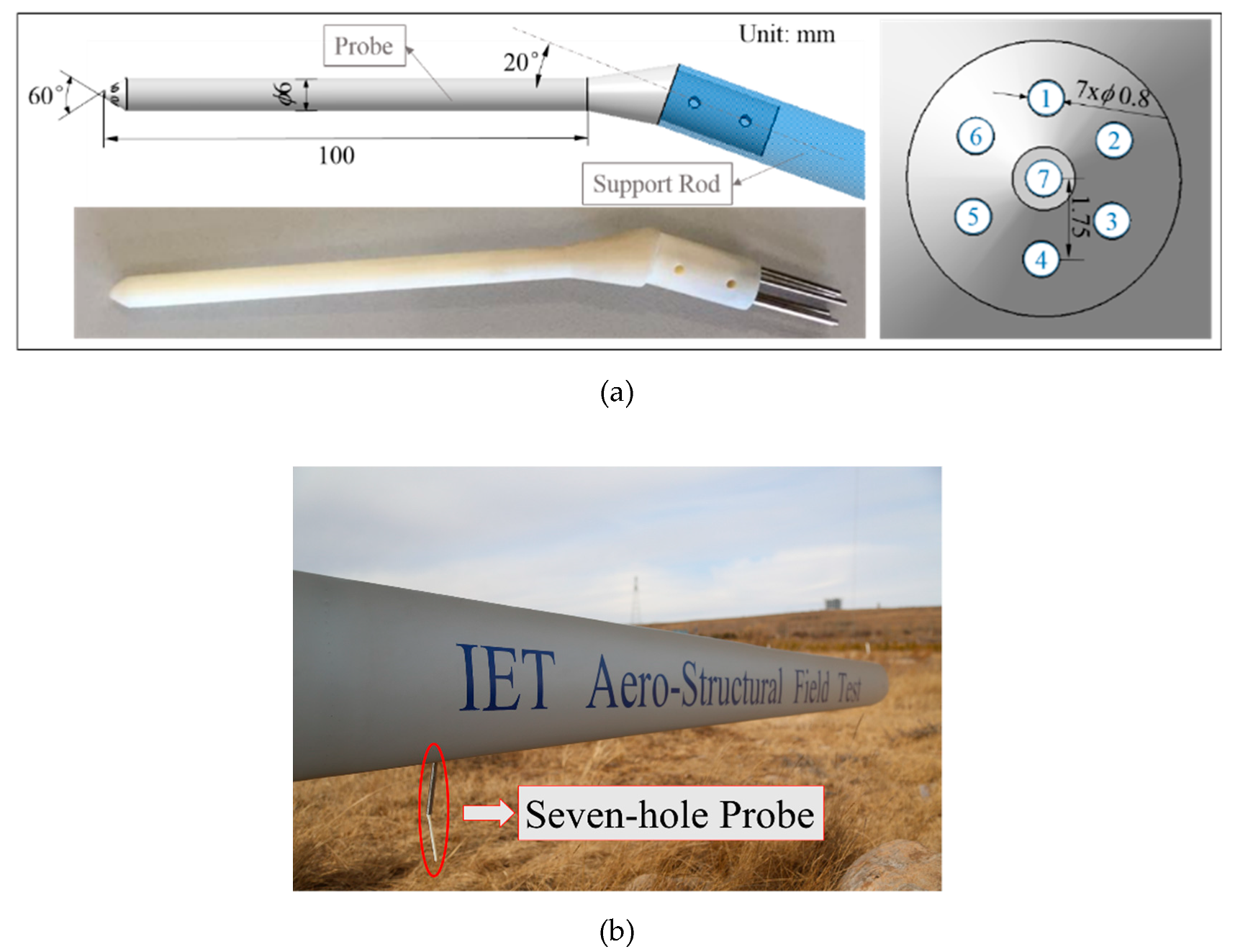
Air probes used in this paper are seven-hole probes developed by Institute of Engineering Thermophysics, which were manufactured by 3D printing. The geometry sizes are shown in Figure 4. The diameter and length of probe fore-body are 6 mm and 100 mm, respectively. The inner diameter of all the holes is 0.8mm with a center-to-center spacing of 1.75 mm. In order to compensate the upwash induction of lift circulation on the flow direction at probe tip, a bending angle of 20° was set at the joint of fore-body and after-body.

All the probes were installed on a customized two degrees of freedom calibration apparatus and calibrated in a 0.5 m by 0.5 m wind tunnel at wind speeds of 10 m/s, 20 m/s, and 30 m/s. Angular range of calibration database is from –50° to 50° for angle of attack and from –50° to 50° for sideslip angle. Finally, the calibration errors for flow angles are lower than 1°, and error for dynamic pressure is lower than 2%, which is shown in

Table 4. Calibration errors of leading-edge probes.

Flow Attribute	Angle of Attack (°)	Sideslip Angle (°)	Dynamic Pressure (%)
Error	0.96	0.77	1.64

.

Each probe was installed at 0.3 m away from corresponding pressure measurement section along the span of blade. After installation, the length of each probe beyond the leading edge is shown in

Table 5. Locations of probe tip.

Probe Name	P1	P2	P3	P4	P5
Span Location (m)	1.798	3.085	4.008	5.122	6.905
Length beyond the leading edge (m)	0.55	0.4	0.345	0.293	0.22

.

3.3. Pressure Distribution Measurement

In order to measure pressure with higher accuracy, the range of pressure sensor should be determined firstly. A better method is to evaluate the maximum flow velocity and the corresponding pressure. The relative inflow speed at blade tip is about 90 m/s when the rotor runs at the rated revolving speed. The corresponding inflow dynamic pressure is about 5000 Pa, according to the deductive Bernoulli equation (Equation (1)):

$$q=\frac{1}{2}\rho V^2$$

(1)

Therefore, the range of pressure sensor should be lower than 10,000 Pa. In addition, the length of pressure tube has a damping effect on the dynamic response of pressure signal. It has been shown [31] experimentally that acoustic damping is small for frequencies up to 40 Hz for a pressure tube with length of 1.1 m and diameter of 1 mm. It requires that location of pressure sensor should be close enough to the pressure taps. With both the above considerations, pressure scanners, ESP-64 with full scale of 1 PSI and measuring accuracy of ±0.05% full scale, manufactured by Measurement Specialties, were purchased and installed in the chamber of a blade, as shown in Figure 5. To facilitate field maintenance and repairs of pressure scanner, three installation windows were manufactured on the pressure side of the blade.

It is difficult to fabricate pressure tap in the large composite wind turbine blades. A method to embed pressure tubes into composite blades during the vacuum assistant resin infusion was developed and applied on the tested blade in this paper. The method has obtained two patents in China. Finally, pressure taps were manufactured at five airfoil sections. The parameters of pressure measurement sections, including airfoil, span location, pressure tap number, and chord, are shown in

Table 6. Parameters of five pressure measurement sections.

Section Name	S1	S2	S3	S4	S5
Airfoil	CAS-W2-450	DU00-W-350	DU97-W-300	DU91-W2-250	DU93-W-210
Span Location (m)	1.498	2.785	3.708	4.822	6.605
Pressure Tap Number	53	57	49	51	46
Chord (m)	0.758	0.658	0.558	0.467	0.369

. The photo of finished aerodynamic measurement blade is shown in Figure 6.

3.4. Synchronous Measurement

Synchronous measurement is to correlate all the parameters sampled, including inflow conditions from anemometer mast, inflow conditions from leading-edge probes, pressure distributions, strains at the blade root, and operating data of wind turbine. The sampling frequency of inflow conditions from anemometer mast is as low as 1 Hz, while it of the other instruments is higher than 50 Hz. Thus, the method of synchronous measurement is to produce a trigger that only ensure the first data of all the parameters sampled is synchronous. In this paper, a synchronizer was customized to trigger all the data acquisition instruments by respective communication protocols, as shown in Figure 7. The time error among first data of all the parameters is less than 20 ms by checking the absolute sampling time.

4. Data Reducing Methods

4.1. Sideslip Angle Correction for Normalization of Pressure Coefficients and Force Coefficients

Usually, pressure coefficients are normalized by Equation (2), where p_i is the surface pressure measured by pressure scanner, p_s and p₀ are the static and total pressure measured by leading-edge probe, respectively:

$$C{p}_i=\frac{p_i-p_s}{p_0-p_s}$$

(2)

However, the relative sideslip angle, β, which is defined in Figure 8, is usually non-zero in the field environment. In non-zero sideslip condition, flow inside of the airfoil plane plays a dominant role in generation of aerodynamic force. So dynamic pressure in Equation (2), $p_0-p_s$, should be corrected as $(p_0-p_s)\cdot {\cos }^2\beta$ in non-zero sideslip condition. The new normalization method is shown in Equation (3):

$$C{p}_i=\frac{p_i-p_s}{(p_0-p_s)\cdot {\cos }^2\beta }$$

(3)

Body-axis forces and their coefficients are calculated by Equations (4) and (5), where N is the normal force perpendicular to the chord, A is the tangential force parallel to the chord, $d{x}_i$, $d{y}_i$ are the interval of pressure taps parallel and perpendicular to the chord respectively, CN is the normal force coefficient, CA is the tangential force coefficient, C is the chord of airfoil:

$$\{\begin{array}{l}A={\displaystyle \sum _{i=1}^N{p}_i\cdot d{y}_i}\\ N={\displaystyle \sum _{i=1}^N{p}_i\cdot d{x}_i}\end{array}$$

(4)

$$\{\begin{array}{l}CA=\frac{{\displaystyle \sum _{i=1}^N{p}_i\cdot d{y}_i}}{\left(p_0-p_s\right)\cdot {\cos }^2\beta \cdot C}={\displaystyle \sum _{i=1}^N\frac{C{p}_i\cdot d{y}_i}{C}}\\ CN=\frac{{\displaystyle \sum _{i=1}^N{p}_i\cdot d{x}_i}}{\left(p_0-p_s\right)\cdot {\cos }^2\beta \cdot C}={\displaystyle \sum _{i=1}^N\frac{C{p}_i\cdot d{x}_i}{C}}\end{array}$$

(5)

Air-axis force coefficients are calculated by body-axis force coefficients according to Equation (6), where Cd is the drag coefficient along the inflow direction, Cl is the lift coefficient perpendicular to the inflow direction, α is the effective angle of attack, as shown in Figure 8:

$$\{\begin{array}{l}Cd=CA\cdot \cos \alpha +CN\cdot \sin \alpha \\ Cl=CN\cdot \cos \alpha -CA\cdot \sin \alpha \end{array}$$

(6)

4.2. Induced Velocity Correction for Determination of the Effective Angle of Attack

The inflow speed and direction measured by probe, $V_p$ and ${\alpha }_p$ are shown in Figure 9. $V_p$ comprises the induced velocity of lift circulation $V_i$ and the undisturbed inflow velocity $V_e$. Effective angle of attack, ${\alpha }_e$, is the angle between the undisturbed inflow velocity $V_e$ and the chord line. Thus, the effective angle of attack at the probe section is corrected by Equation (7):

$${\alpha }_e={\alpha }_p-{\alpha }_i$$

(7)

The iteration steps to calculate ${\alpha }_e$ are shown in Figure 10.

Step 1: Assume the angle of attack measured by probe, ${\alpha }_p$, is the initial angle of attack, and calculate the sectional lift by integration of the pressure distribution and Equation (6).

Step 2: Compute the lift circulation by the Kutta–Joukowski theorem, as shown in Equation (8), where $V_p$ is the inflow speed measured by probe, $\beta$ is sideslip angle measured by probe, $L$ is the sectional lift calculated by Step 1, and $\rho$ is the air density measured by atmospheric pressure and temperature meters:

$$\mathsf{\Gamma }=\frac{L}{\rho V_p\cos \beta }$$

(8)

Step 3: Let us consider the blade as a lift line and compute the induced velocity, $V_i$, by the Biot–Savart integral law, as shown in Equation (9), where $\left|AB\right|$ is the distance between probe tip to lift line, and $a_1$, $a_2$ are shown in Figure 11:

$$V_i=\frac{\mathsf{\Gamma }}{4\pi \left|AB\right|}\left(\cos a_1+\cos a_2\right)$$

(9)

Step 4: Compute the new inflow velocity, $V_n$, by velocity resolution of $V_p$ and $V_i$, and compute the new angle of attack, ${\alpha }_n$.

Step 5: Calculate the error between the new angle of attack and the initial angle of attack used in Step 1. If the error is less than 0.1°, the effective angle of attack is equal to the new angle of attack. If not, repeat Steps 1 to 4, replacing the initial angle of attack with the new angle of attack.

5. Results and Discussions

5.1. Field Test Cases Selection

The direct validation method is to compare the aerodynamic performance of blade section measured in the field with the 2D airfoil data measured in a wind tunnel. Thus, the testing conditions between field measurement and 2D wind tunnel measurement should be similar as much as possible. However, there exists some differences between field measurement on the 3D blade and wind tunnel measurement on the 2D airfoil. Firstly, tip and root vortices over a blade with finite length will have a 3D induction effect on the flow over the entire blade. Additionally, the airfoil and twist angle along the blade span are different, which will have another 3D effect. Secondly, for a rotating blade, stall delay effects [10] are remarkable, especially for the blade root. Finally, wind turbine usually operates in yaw and high turbulent density conditions due to the unsteady atmospheric inflow.

Therefore, to minimize the 3D induction effect, aerodynamic data of DU93-W-210 airfoil, located at the mid-span in Table 3, were chosen to compare. In addition, for eliminating the stall delay effects, the aerodynamic data were sampled when the wind turbine was shutdown.

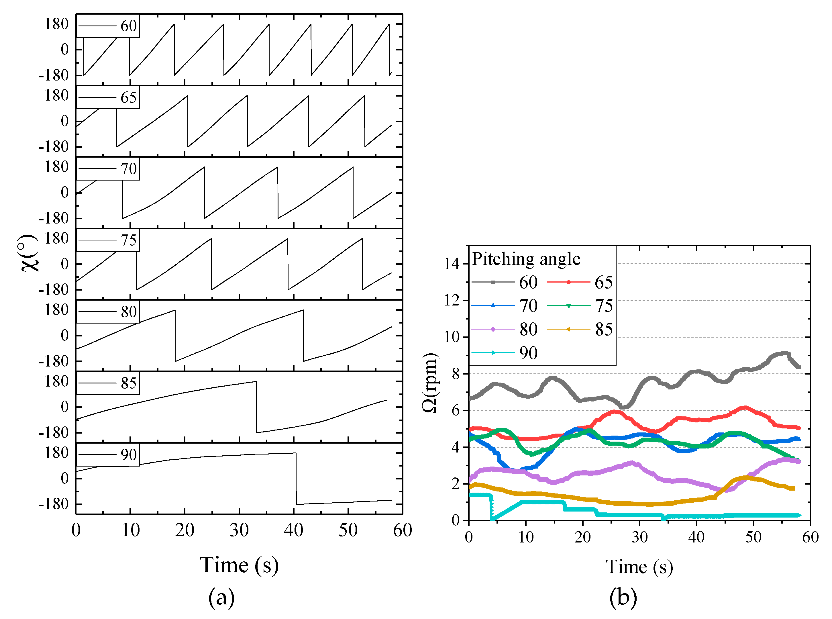
The testing cases are shown in

Table 7. The testing cases to compare with the 2D wind tunnel.

Case	Status of Turbine	Pitching Angle (°)	Sampling Frequency (Hz)	Sampling Time (sec)
1	Stop	60	50	60
2	Stop	65	50	60
3	Stop	70	50	60
4	Stop	75	50	60
5	Stop	80	50	60
6	Stop	85	50	60
7	Stop	90	50	60

, where pitching angles are changed from 60° to 90° with interval of 5°, sampling frequency is 50 Hz and sampling time is 60 s. In this paper, the pitching angle is 90° when the leading edge of the blade points to upstream of the inflow.

Azimuth angle of rotor, $\chi$, is the angle between pitch axis of the blade with pressure taps and tower axis. Yaw angle of wind turbine, $\gamma$, is the angle between inflow direction and rotating axis of rotor. Yaw angle is positive when the freestream comes from left side of the wind turbine. The definitions are shown in Figure 12.

The inflow conditions at the nacelle are shown in Figure 13. It is observed that inflow speed varies in the 8 m/s to 12 m/s ranges, and yaw angle varies in the –20° to 0°. In the sampling time of 60 s, both magnitude and direction of inflow vary significantly, which is the third difference from the 2D wind tunnel measurement as is mentioned previously.

When the wind turbine is shutdown, the rotor is still free to rotate, although rotor speed is very low. It is shown from Figure 14 that rotor speed increases with the decrease of pitching angle. The maximum rotor speed is about 9 rpm at a pitching angle of 60°, which is much lower than rated rotor speed of 62 rpm. In these testing cases, rotor can be regarded as quasi-static, and stall delay effects due to rotating is weak enough to be ignored.

5.2. Angle-Averaged Processing Method

Instantaneous lift coefficient calculated by Equation (6) and angle of attack calculated by Equation (7) at each sampling time were plotted as scattered points in Figure 15. It is shown that the distributions of the scattered point are almost overlapped at all the pitching angles.

However, it is difficult to determine relationship between lift coefficient and angle of attack, because each angle of attack corresponds to a number of lift coefficient values. An angle-averaged method was employed to process the multi-value lift coefficient at one angle of attack to single-value. In the angle-averaged method, all the angles of attack were divided into several data sets with the length of 1°. Each angle of attack set is ${\alpha }_k=\left[{\alpha }_{k1},{\alpha }_{k2},\dots {\alpha }_{kn}\right]$, and the corresponding lift coefficient dataset is $C{l}_k=\left[C{l}_{k1},C{l}_{k2},\dots C{l}_{kn}\right]$. Then the lift coefficients and angles of attack in each dataset were averaged to obtain the angle-averaged lift coefficient and angle of attack, as shown in Equation (10), where i = 1, 2,… n.

$$\{\begin{array}{c}{\alpha }_k=\frac{{\displaystyle \sum _{i=1}^n{\alpha }_{ki}}}{n}\\ C{l}_k=\frac{{\displaystyle \sum _{i=1}^{n}C{l}_{ki}}}{n}\end{array}$$

(10)

The relationship curves of angle-averaged lift coefficient and angle of attack are shown in Figure 16a. All the curves at different pitching angles are almost overlapped also. Thus, the cases at the different pitching angle can be regarded as one case to simplify the data analysis. Finally, the instantaneous data of all the cases at different pitching angles was angle-averaged to plot in one curve, as shown in Figure 16b.

5.3. Comparison with 2D Wind Tunnel Data

In order to minimize the 3D induction effect from blade root and tip, aerodynamic data of DU93-W-210 airfoil at r/R = 0.64 of the blade was chosen to compare with the 2D wind tunnel data, where R is the radius of rotor. The Reynolds number was computed by Equation (11), where V is the velocity measured by the corresponding seven-hole probe, P and T are the atmospheric pressure and temperature measured by the corresponding sensor on the upstream anemometer mast, R is the ideal gas constant, $\mu (T)$ is the kinetic viscosity calculated by Sutherland’s law. The obvious fluctuations of Reynolds number can be observed in Figure 17. However, the mean Reynolds number is about 2 × 10⁵ at the test cases.

$$\mathrm{Re}=\frac{\rho Vl}{\mu }=\frac{P}{RT}\cdot \frac{Vl}{\mu \left(T\right)}$$

(11)

Wind tunnel data of DU93-W-210 airfoil is from Mie University [32]. The measurements were performed in the low-speed wind tunnel with a maximum velocity of 52 m/s, and a measurement section size of 0.65 × 0.65 × 2.0 m. The turbulence intensity is less than 0.15% at the test section. The experimental wind speed was at 30m/s corresponding to a Reynolds number of Re = 3.5 × 10⁵, which is the most proximate inflow conditions with the field conditions that can be found in the literatures. More detailed information about the wind tunnel measurements can be found in Kamada’s work [32].

Three methods were applied to investigate the effects of sideslip angle and induced velocity on the relationship between the lift coefficient and angle of attack. As is shown in

Table 8. Computation methods of angle of attack.

	Method I	Method II	Method III
Sideslip angle correction	●	○	●
Induced velocity correction	○	●	●

, only sideslip angle correction for normalization of aerodynamic coefficients was taken into account in Method I. Only the induced velocity correction for the determination of the effective angle of attack was applied in Method II. In Method III, both corrections were applied.

The relationship curves between lift coefficient and angle of attack with the three methods were plotted in Figure 18 and compared with wind tunnel data from Mie University [32]. It can be shown that good agreements are achieved between field data using Method III and wind tunnel data, especially at an angle of attack less than 8°. However, remarkable deviations are observed when Method I was applied. The slope of relationship curve between lift coefficient and angle of attack is clearly lower. It means that induced velocity from lift circulation has appreciable impact on the directly measured velocity by leading-edge probes. When determining the angle of attack in the field, induced velocity correction must be taken into account. When Method II was applied, both Method II and Method III give almost similar results at angles of attack less than 10°. It means that the sideslip angle has little impact on the relationship between the lift coefficient and the angle of attack.

Furthermore, pressure coefficients of the field measurements, angle-averaged with the data of all the testing cases, were further compared with the wind tunnel data in detail. It is shown from Figure 19 that between two angles of attack, 6° and 12°, the shapes of the pressure distributions are different, and at each angle of attack, the pressure distribution of the field measurement has good agreement with the wind tunnel data.

In summary, good agreements are achieved for the lift and pressure coefficients between the field measurements and 2D wind tunnel measurements, which verifies that the designation, implementation, and data reducing methods of the aerodynamic field measurement platform developed in this paper are reasonable and reliable.

To evaluate the dispersion of instantaneous lift coefficients in Figure 15, the standard deviations were calculated by Equation (12), where n is the sample size of the lift coefficient dataset, Cl_k is the angle-averaged lift coefficient defined in Equation (11). Figure 20 shows standard deviations of lift coefficient at different angle-average angles of attack, which are about 0.2. This means that the natural inflow condition in the field will introduce about standard deviation of 0.2 for lift coefficient when aerodynamic loads are predicted by aerodynamic data from 2D wind tunnel tests. In order to investigate the source of the dispersion of instantaneous lift coefficients, aerodynamic data in time history were analyzed further:

$$\sigma \left(C{l}_k\right)=\sqrt{\frac{1}{n}{\displaystyle \sum _{i=1}^n{\left(C{l}_{ki}-C{l}_k\right)}^2}}$$

(12)

5.4. Time History Analysis for the Dispersion of Instantaneous Lift Coefficients

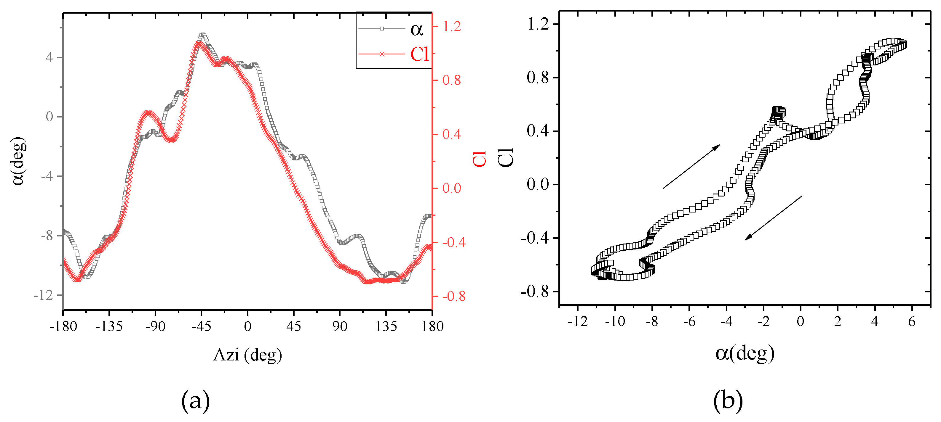
Although good agreements has been achieved for both angle-averaged lift and pressure coefficients from Figure 18 and Figure 19, remarkable dispersion can be observed for instantaneous lift coefficients from Figure 15 and Figure 20. Time history of azimuth angle, angle of attack, and lift coefficient in Case 1, where the pitching angle is 60°, were analyzed and shown in Figure 21. It can be observed that both the lift coefficient and the angle of attack vary quasi-periodically, and the frequencies are same with azimuth angle. For this reason, aerodynamic behaviors in one rotation period were discussed. It is shown from Figure 22a that both the angle of attack and lift coefficient are largest when the tested blade rotates across the bottom of rotor corresponding to azimuth angle of 0°, while they are lowest when the tested blade rotates across the top of rotor corresponding to azimuth angle of 180° or –180°. In one rotation period, remarkable dynamic response phenomenon can be observed from Figure 22b. A clockwise hysteresis loop of lift coefficients was formed when angles of attack increased from –12° to 6° and decreased from 6° to –12°. Obviously, the dynamic response make instantaneous lift coefficients at the same angle of attack dispersive.

The reason that causes the quasi-periodically variation of angle of attack is investigated also in the present research. A comparison between yaw angle and variation amplitude of angle of attack is shown in Figure 23, where amplitude of angle of attack was multiplied by –1 to make a direct contrast with yaw angle. It can be observed that variation amplitude of angle of attack is closely correlated with yaw angle, although certain irregular deviations exists at some instantaneous time. As a whole, the variation amplitudes are determined by the yaw angles.

If yaw angle is negative, angle of attack will be largest when the tested blade rotates across the bottom of rotor at azimuth angle of 0°. It can also be deduced that if yaw angle is positive, angle of attack will be lowest when the tested blade is at azimuth angle of 0°. The quasi-periodically variation of the angle of attack caused by the yawing angle, induces dynamic response of a clockwise hysteresis loop in the lift coefficient. The dynamic response is the main source of the dispersion of instantaneous lift coefficients with a standard deviation of 0.2.

6. Conclusions and Future Research

An aerodynamic measurement platform in the field was developed based on a horizontal axis wind turbine from IET in China in this paper to study the measuring and analyzing method of the angle of attack. Five seven-hole probes were installed at the leading edge to measure inflow conditions at the near field, which is very important to improve the measuring accuracy of actual inflow conditions over the blades, and provide the static and total pressure for data normalization. Two data reducing processes, sideslip angle correction and induced velocity correction, were proposed to determine the effective angle of attack. An angle-averaged processing method was employed to investigate the single-valued relationship between lift coefficient of blade section and angle of attack. As a result, good agreements are achieved for angle-averaged lift and pressure coefficients between field and 2D wind tunnel measurement. Without consideration of induced velocity by lift circulation, the slope of Cl ~ α curve will be clearly lower.

In the field, angle of attack varies quasi-periodically with the rotation of rotor in field, which is caused by yaw angle of inflow. The variation amplitudes of angle of attack are determined by the yaw angles. The variation of angle of attack induces dynamic response of a clockwise hysteresis loop in the lift coefficient. The dynamic response is the main source of a dispersion of instantaneous lift coefficients with a standard deviation of 0.2.

References

- Shen, X.; Zhu, X.; Du, Z. Wind turbine aerodynamics and loads control in wind shear flow. Energy 2011, 36, 1424–1434. [Google Scholar] [CrossRef]
- Li, L.; Liu, Y.; Yuan, Z.; Gao, Y. Wind field effect on the power generation and aerodynamic performance of offshore floating wind turbines. Energy 2018, 157, 379–390. [Google Scholar] [CrossRef]
- Gould, B.J.; Burris, D.L. Effects of wind shear on wind turbine rotor loads and planetary bearing reliability. Wind Energy 2016, 19, 1011–1021. [Google Scholar] [CrossRef]
- Sezer-Uzol, N.; Uzol, O. Effect of steady and transient wind shear on the wake structure and performance of a horizontal axis wind turbine rotor. Wind Energy 2013, 16, 1–17. [Google Scholar] [CrossRef]
- Li, Q.A.; Murata, J.; Endo, M.; Maeda, T.; Kamada, Y. Experimental and numerical investigation of the effect of turbulent inflow on a Horizontal Axis Wind Turbine (Part I: Power performance). Energy 2016, 113, 713–722. [Google Scholar] [CrossRef]
- Li, Q.A.; Kamada, Y.; Maeda, T.; Murata, J.; Yusuke, N. Effect of turbulence on power performance of a Horizontal Axis Wind Turbine in yawed and no-yawed flow conditions. Energy 2016, 109, 703–711. [Google Scholar] [CrossRef]
- Li, Q.A.; Kamada, Y.; Maeda, T.; Murata, J.; Nishida, Y. Effect of turbulent inflows on airfoil performance for a Horizontal Axis Wind Turbine at low Reynolds numbers (part I: Static pressure measurement). Energy 2016, 111, 701–712. [Google Scholar] [CrossRef]
- Madsen, H.A.; Mikkelsen, R.; Øye, S.; Bak, C.; Johansen, J. A Detailed investigation of the Blade Element Momentum (BEM) model based on analytical and numerical results and proposal for modifications of the BEM model. J. Phys. Conf. Ser. 2007, 75, 012016. [Google Scholar] [CrossRef]
- Simms, D.A.; Schreck, S.; Hand, M.; Fingersh, L. NREL Unsteady Aerodynamics Experiment in the NASA-Ames Wind Tunnel: A Comparison of Predictions to Measurements; National Renewable Energy Lab.: Golden, CO, USA, 2001.
- Breton, S.P.; Coton, F.N.; Moe, G. A study on rotational effects and different stall delay models using a prescribed wake vortex scheme and NREL phase VI experiment data. Wind Energy 2008, 11, 459–482. [Google Scholar] [CrossRef]
- Snel, H.; Houwink, R.; Bosschers, J. Sectional Prediction of Lift Coefficients on Rotating Wind Turbine Blades in Stall; ECN-C--93-052; Netherlands Energy Research Foundation: Petten, The Netherlands, 1994. [Google Scholar]
- Du, Z.; Selig, M. A 3-D stall-delay model for horizontal axis wind turbine performance prediction. In Proceedings of the 1998 ASME Wind Energy Symposium, Reno, NV, USA, 12–15 January 1998. [Google Scholar]
- Leishman, J.; Beddoes, T. A Semi-Empirical Model for Dynamic Stall. J. Am. Helicopter Soc. 1989, 34, 3–17. [Google Scholar] [CrossRef]
- Sheng, W.; Galbraith, R.A.M.; Coton, F.N. A Modified Dynamic Stall Model for Low Mach Numbers. J. Solar Energy Eng. 2008, 130, 1–10. [Google Scholar] [CrossRef]
- Mulleners, K.; Raffel, M. The Onset of Dynamic Stall Revisited. Exp. Fluids 2012, 52, 779–793. [Google Scholar] [CrossRef]
- Tangler, J. Horizontal-Axis Wind-System Rotor Performance Model Comparison: A Compendium; NASA STI/Recon Technical Report N83; NASA: Washington, DC, USA, 1983.
- Butterfield, C.; Nelsen, E. Aerodynamic Testing of a Rotating Wind Turbine Blade; SERI/TP-257-3490; Solar Energy Research Inst.: Golden, CO, USA, 1990. [Google Scholar]
- Butterfield, C.; Musial, W.; Simms, D. Combined Experiment Phase I. Final Report; NREL/TP-257-4655; National Renewable Energy Lab.: Golden, CO, USA, 1992.
- Butterfield, C.P.; Musial, W.; Scott, G.; Simms, D. NREL Combined Experimental Final Report—Phase II; NREL/TP-442-4807; National Renewable Energy Lab.(NREL): Golden, CO, USA, 1992.
- Simms, D.A.; Hand, M.; Fingersh, L.; Jager, D. Unsteady Aerodynamics Experiment Phases II-IV Test Configurations and Available Data Campaigns; NREL/TP-500-25950; National Renewable Energy Laboratory: Golden, CO, USA, 1999.
- Simms, D.; Hand, M.M.; Fingersh, L.; Jager, D.; Cotrell, J.; Schreck, S.; Larwood, S. Unsteady Aerodynamics Experiment Phase V: Test Configuration and Available Data Campaigns; TOPICAL; National Renewable Energy Lab: Golden, CO, USA, 2001.
- Aagaard Madsen, H. Aerodynamics of a Horizontal-Axis Wind Turbine in Natural Conditions; Risøo National Laboratory: Roskilde, Denmark, 1991.
- Brand, A.; Dekker, J.; de Groot, C.; Späth, M. Field rotor-aerodynamics-The rotating case. In Proceedings of the 35th Aerospace Sciences Meeting and Exhibit, Reno, NV, USA, 6–9 January 1997. [Google Scholar]
- Bruining, A. Aerodynamics Characteristics of a 10 m Diameter Rotating Wind Turbine Blade; IW-084R; Delft University of Technology: Delft, The Netherlands, 1996. [Google Scholar]
- Schepers, J.; Brand, A.; Bruining, A.; Graham, J.; Hand, M.; Infield, D.; Madsen, H.; Paynter, R.; Simms, D. Final Report of IEA An-nex XIV: Field Rotor Aero-Dynamics; ECN-C--97-027; Energieonderzoek Centrum Nederland: Petten, The Netherlands, 1997. [Google Scholar]
- Schepers, J.; Brand, A.; Bruining, A.; Hand, M.; Infield, D.; Madsen, H.; Maeda, T.; Paynter, J.; van Rooij, R.; Shimizu, Y. Final Report of IEA Annex XVIII Enhanced Field Rotor Aerodynamics Database; ECN-C-02-016; Energy Research Center of the Netherlands: Petten, The Netherlands, 2002. [Google Scholar]
- Aagaard Madsen, H.; Bak, C.; Schmidt Paulsen, U.; Gaunaa, M.; Fuglsang, P.; Romblad, J.; Olesen, N.A.; Enevoldsen, P.; Laursen, J.; Jensen, L. The DAN-AERO MW Experiments: Final Report; Danmarks Tekniske Universitet, Risø Nationallaboratoriet for Bæredygtig Energi: Lyngby, Denmark, 2010. [Google Scholar]
- Li, D.S.; Guo, T.; Li, Y.R.; Hu, J.S.; Zheng, Z.; Li, Y.; Di, Y.J.; Hu, W.R.; Li, R.N. Interaction between the atmospheric boundary layer and a standalone wind turbine in Gansu—Part I: Field measurement. Sci. China Phys. Mech. Astron. 2018, 61, 1–14. [Google Scholar] [CrossRef]
- Shen, W.Z.; Hansen, M.O.; Sørensen, J.N. Determination of the angle of attack on rotor blades. Wind Energy 2009, 12, 91–98. [Google Scholar] [CrossRef]
- Morote, J. Angle of attack distribution on wind turbines in yawed flow. Wind Energy 2016, 19, 681–702. [Google Scholar] [CrossRef]
- Späth, M.; Stefanatos, N. Survey on Frequency Responses of Pressure Tubes Installed in a 12.5 Meter Rotor Blade; Netherlands Energy Research Foundation ECN: Petten, The Netherlands, 1992. [Google Scholar]
- Kamada, Y.; Maeda, T.; Murata, J.; Toki, T.; Tobuchi, A. Effects of turbulence intensity on dynamic characteristics of wind turbine airfoil. J. Fluid Sci. Technol. 2011, 6, 333–341. [Google Scholar] [CrossRef]
Figure 1.
Google map of the wind farm.
Figure 2.
Photo and parameters of the 100 kW wind turbine.
Figure 3.
Overall layout of field measurement platform.
Figure 4.
(a) Geometry of seven-hole probe, and (b) photo of the probe at the leading edge.
Figure 5.
(a) Sketch diagram, and (b) photo of surface pressure measurement system on blades.
Figure 6.
Photo of the tested blade.
Figure 7.
The measuring and controlling system.
Figure 8.
Sketch diagram of the body-axis and air-axis force.
Figure 9.
Effective angle of attack measured by leading-edge probe.
Figure 10.
The flowchart to calculate the effective angle of attack.
Figure 11.
Biot–Savart integral law.
Figure 12.
Definitions of azimuth angle of rotor and yaw angle of wind turbine.
Figure 13.
Inflow speed (a) and yaw angle (b) at the nacelle in the testing cases.
Figure 14.
Time history of azimuth angle (a) and rotor speed (b) in the testing cases.
Figure 15.
Instantaneous lift coefficients at r/R = 0.64 with different pitching angles.
Figure 16.
Angle-averaged lift coefficients from each pitching angle case (a) and all the cases (b).
Figure 17.
Reynolds number range at different pitching angle cases.
Figure 18.
Comparison of lift coefficients of DU93-W-210 between the field test and 2D wind tunnel test.
Figure 19.
Comparison of pressure coefficients: (a) α = 6°, (b) α = 12°.
Figure 20.
Standard deviations of the lift coefficient.
Figure 21.
Time history of azimuth angle, angle of attack, and lift coefficient in Case 1.
Figure 22.
(a) The variation of angle of attack and lift coefficient in one rotation period, and (b) dynamic response of lift coefficient varying with the angle of attack.
Figure 23.
Comparison of yaw angle and variation amplitude of angle of attack measured by probe in Case 1.