Abstract
Ultrashort pulses are severely distorted even by low dispersive media. While the mathematical analysis of dispersion is well known, the technical literature focuses on pulses, Gaussian and Airy pulses, which keep their shape. However, the cases where the shape of the pulse is unaffected by dispersion is the exception rather than the norm. It is the objective of this paper to present a variety of pulse profiles, which have analytical expressions but can simulate real-physical pulses with great accuracy. In particular, the dynamics of smooth rectangular pulses, physical Nyquist-Sinc pulses, and slowly rising but sharply decaying ones (and vice versa) are presented. Besides the usage of this paper as a handbook of analytical expressions for pulse propagations in a dispersive medium, there are several new findings. The main findings are the analytical expressions for the propagation of chirped rectangular pulses, which converge to extremely short pulses; an analytical approximation for the propagation of super-Gaussian pulses; the propagation of the Nyquist-Sinc Pulse with smooth spectral boundaries; and an analytical expression for a physical realization of an attenuation compensating Airy pulse.
1. Introduction
Ultrashort pulses are ubiquitous in numerous applications including in bio- and medical-imaging (see, for example, [1,2,3]), optical communications (see, for example, [4,5]), and microscopy (see, for example, Ref. [6,7]), etc.
One of the clear shortcomings of short pulses is the consequences of their wide spectrum. When the spectrum is spectrally wide, the absorption variations within the spectrum increases. However, even if the absorption is approximately homogenous within the pulse spectral range, the refraction index is wavelength-dependent and therefore the pulse experiences dispersion effects.
Dispersion occurs whenever each one of the pulse’s spectral components propagates with a different velocity. Consequently, the pulse experiences shape distortions. The temporally shorter the pulse, the larger the distortions. Moreover, while the dispersion effects are proportional to the medium’s length, it is inversely proportional to the square of the pulse’s temporal width; therefore, ultra-short pulses are prone to being affected by dispersion even in relatively short media [8,9,10].
Clearly, most of the dispersion mitigation techniques were implemented in the optical communication arena, where dispersion can have a destructive effect on the transmitting signals. It has been shown that via ordinary smf28 fiber (the most ubiquitous fiber type) it is impossible to decode data, which is transmitted at a 10 Gb/s rate, beyond a distance of 160 km (see Ref. [11] and in the quantum analogy see Ref. [12]). Clearly, in the presence of noise, this distance shrinks substantially. If the data is carried by picosecond pulses (which is only 1% of the temporal width of the 10 Gb/s signal’s individual pulses), this maximum distance is reduced to merely 16 m, and the distortion effects will be felt within less than a meter. In the femtosecond domain, the dispersion effects are, using the terminology and example of Ref. [13], more dramatic: A 10 fs laser pulse in the 800 nm spectral regime, which propagates through 4 mm of BK7 glass, will be temporally broadened to 50 fs.
It is well known that dispersion is governed by the dispersion equation, which can easily be solved numerically. However, to evaluate the effects of dispersion and to predict them, some intuition is required. In most textbooks, Gaussian pulses are used as a litmus tool to predict the dispersion effect [8,13,14]. Gaussian pulses are very useful since, on the one hand, they are localized pulses with a well-defined width and energy, and on the other hand, the shape of their spectrum is mathematically similar to the dispersion effect. Therefore, the propagation of Gaussian pulses in dispersion medium has a relatively simple analytical solution. This simple pulse model can be used to qualitatively evaluate some fundamental limitations. However, it fails in quantifying their values (see Ref. [11] and the references therein). In fact, the Gaussian model predicts that the pulse keeps its Gaussian shape, and its width is proportional to the square root of the elapsed period. This conduct resembles the spatial spreading of a Gaussian distribution of particles in a diffusion process [15]. Since the “particle” realization of the dispersion process is common in the popular description of chromatic dispersion, the similarity to diffusion may be misleading, since, in fact, this similarity appears only in the Gaussian scenario. Whenever the initial pulse profile deviates from the Gaussian’s one, the differences between diffusion and dispersion are clearly shown. In general, the two processes tend to smooth out the signal. However, the processes are fundamentally different, and the main differences appear after short distances. This discrepancy clearly appears in most optical communication protocols, where the pulses never have Gaussian profiles. Consequently, the signal distortion is completely different from the Gaussian analysis predictions. To overcome this problem, super-Gaussian pulses are commonly used to model real communications scenarios [16,17,18]. Despite the fact that super-Gaussian pulses are much better approximation to real pulses, they have two weaknesses: they cannot be implemented in Non-Return-to-Zero (NRZ) protocols and they do not have a close-form analytical solution.
It is the objective of this paper to assemble important pulses profile, whose propagation in dispersive medium can be expressed in analytical terms. It is shown that there are profiles, which are much better candidates to simulate real pulses, but their dynamics can be formulated in a closed-form analytical expressions.
Moreover, it is shown that the dynamics of almost any practical pulse profile in dispersive media can be simulated and approximated by analytical expressions.
In the first part of the paper, after the introduction of the general theory (Section 2) and the presentation of fundamental theorems (Section 3), the propagation of a Gaussian pulse is presented (Section 4). In the second part, it is shown that it is possible to present, analytically, the propagation of singular pulses (Section 5), which can be written initially with exponentials and step functions (like rectangular pulses and exponential-step pulses). In the third part, it is shown that every step function can be replaced with a smooth step function, and therefore any singular pulse, which is presented in the previous part of the paper, can be replaced with its counterpart smooth version (Section 6). In particular, smooth rectangular pulses can replace super-Gaussian ones. The fourth part is dedicated to the important pulse, which is singular in the spectral domain, i.e., the Nyquist-Sinc pulse (Section 7). First, the analytical expression for its propagation in dispersive medium is presented, and then the analytical expression of the propagation of its spectrally-smooth, i.e., physical, counterpart is presented as well. In the last part of the paper, accelerated-Airy pulses and attenuation compensating pulses are presented, as well as their physical counterparts (Section 8).
2. Generic Dispersion Analysis
Let represent the envelope of an electromagnetic (EM) pulse, which propagates in the z-direction in a dispersive medium with the dispersion coefficient , and thus obeys the following equation [14]:
where is the time in a frame of reference that travels at the velocity of light in the medium (, where is the vacuum light’s velocity, and is the mean refractive index), i.e., is the real time. This equation is valid provided all spectral components of the pulse are governed by the following dispersion relation:
If is the initial pulse profile, then the pulse profile at the end of the medium can be evaluated by the following convolution:
where the dispersion Kernel (see Appendix A) is
3. Fundamental Dispersion Theorems
To analyze the dispersion dynamics of the different pulses, we need some analytical tools, which will be formulated as the following theorems.
3.1. Pulse Boosting and Decaying
Let be an initial pulse whose dispersive dynamics is known, i.e., at the end of the dispersive medium its profile is also given as . Then, if the initial pulse is boosted by shifting the pulse’s spectrum, i.e., by multiplying the profile by a harmonic function:
then the pulse’s profile at the end of the medium (after a distance ) is (see Appendix B)
Clearly, this theorem can be generalized to the case where the initial pulse is multiplied by an exponent:
where can be any real, imaginary, or complex number. In which case, if the initial function does not diverge, the solution at the end of the medium is
3.2. Pulse Chirping
Let be an initial pulse whose dispersive dynamics is known, i.e., at the end of the dispersive medium, its profile is ; then, if the initial pulse is chirped, i.e.,:
for any real q, the pulse’s profile at the end of the medium (after a distance z) is (see Appendix C)
Again, this theorem can be generalized to the case where the initial profile is multiplied by a generic Gaussian. That is, if the initial pulse is
where can be any complex number, then as long as , the solution at the end of the medium is
4. Gaussian Pulse
The simplest pulse, which is ubiquitous in the literature, is the Gaussian one. This is one of the few cases where the pulse has the same shape as its Fourier Transform. Therefore, since the dispersion dynamics can be formulated as a convolution with a complex Gaussian (Equation (4)), then in general, the pulse profile remains a complex Gaussian. In this case, the initial pulse profile is
and thus the pulse’s profile at the end of the dispersive medium is (following Equation (12))
The profile of Equation (14) is plotted in Figure 1 and a spatiotemporal presentation of its intensity is presented in Figure 2. Hereinafter, we adopt the following dimensionless parameters: and .
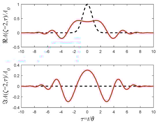
Figure 1.
The real (upper panel) and imaginary (lower panel) components of the pulse (Equation (14)). The dashed curve represents the initial profile (for ), while the solid curve represents the signal after a distance, which corresponds to . Time is measured in units of , which corresponds to the pulse’s temporal width.
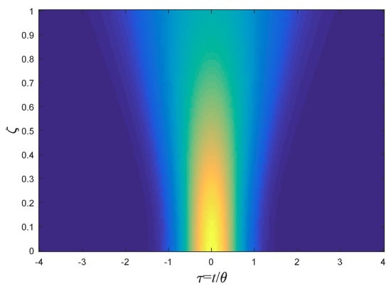
Figure 2.
A false-color presentation of the pulse’s intensity (Equation (14)) as a function of the normalized time and the normalized distance .
Sample Application: The pulses that many mode locked lasers emit can be simulated by Gaussian pulses (see Ref. [14]). When such a pulse with a Full Width at High Maximum (FWHM) of 1 ps (which corresponds to ) and a carrier wavelength of enters a BK7 glass, then , and in Figure 2 corresponds to .
4.1. Boosted Gaussian
When the initial pulse is a boosted Gaussian,
then using Relation (6), the final (after a distance z) profile is
which means that beside the pulse spreading, the pulse’s peak propagates with reciprocal “velocity” . The larger the spectral shift , the larger the temporal shift of the pulse. The pulse’s profile and its intensity’s dynamics are presented in Figure 3 and Figure 4, respectively.
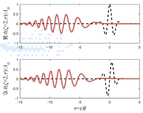
Figure 3.
The real (upper panel) and imaginary (lower panel) components of the Gaussian pulse (Equation (16)). The dashed curve represents the initial profile (for ), while the solid curve represents its final shape (for ). In this example, the carrier frequency is .
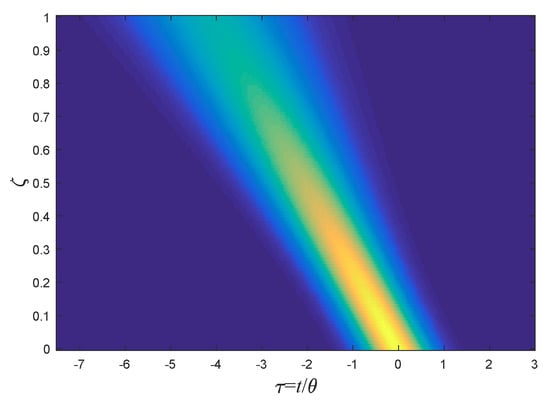
Figure 4.
Same as Figure 2, but for the intensity () of the pulse presented by Equation (16). (In this example, ).
4.2. Chirped Gaussian
When the initial pulse is chirped, i.e., the pulse’s phase has an additional quadratic dependence on time, i.e.,
then, using Equation (10) the final pulse is
In Figure 5, the temporal dynamics of the pulse (Equation (18)) is presented for the same parameters as Figure 2 but with additional . The shrinkage of the pulse’s width is clearly shown, which is a consequence of the fact that the chirping has widened the spectral width of the initial pulse.
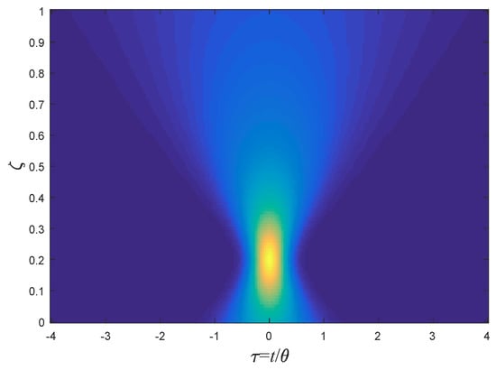
Figure 5.
Same as Figure 2, but for the intensity () of the pulse presented by Equation (18) (in this example, ).
5. Singular Pulses
Before going into the propagation of profiles, which can simulate real pulses, it is instructive to investigate a family of pulses with singularity points. The singularity points are points in which either the pulse’s amplitude or its derivatives are discontinuous. Despite their singularities, these pulses can simulate pulses which have sharp boundaries. Moreover, it will be shown that these generalized, i.e., singular, pulses can be modified very simply into smooth ones and therefore can be implemented in real, physical scenarios.
5.1. The Step Function
The step function response of a dispersive medium is related to the complex error function. Let the initial pulse’s profile be a step function, i.e.,
where is the Heaviside step-function, then the pulse at the end of the medium is
Clearly, if initially
then
Similarly, using Equation (6), the initial boosted step function pulse
will propagate to read
This result is known in the literature as Moshinsky’s function. In quantum mechanics, this function was used to simulate an electrons’ beam, which was blocked by a beam shutter [19,20]. In the quantum analogy, the wavefunction exhibits interference in time.
5.2. Rectangular Pulses
The fundamental generalized pulse is the rectangular one. Unlike the delta function, the rectangular pulse has a finite energy and therefore can simulate real pulses in many scenarios despite its singular edges (a real rectangular pulse), and therefore it is ubiquitous in the literature.
The rectangular pulse can be written with the aid of the step function or the rectangular function:
where
Equation (25) has two singular points () in which the pulse’s amplitude is discontinuous. The dynamics of this rectangular pulse can be formulated analytically:
In Figure 6, the real and imaginary components of (27) are plotted for two different medium’s length. The ripples in the pulse’s profile appear after a very short distance.
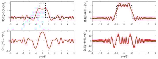
Figure 6.
The real (upper panel) and imaginary (lower panel) components of the rectangular pulse (Equation (27)). The dashed curve represents the initial profile (for ), while the solid curve represents its final shape (for on the right and on the left).
In Figure 7, a spatiotemporal intensity plot (as a function of and ) is presented.
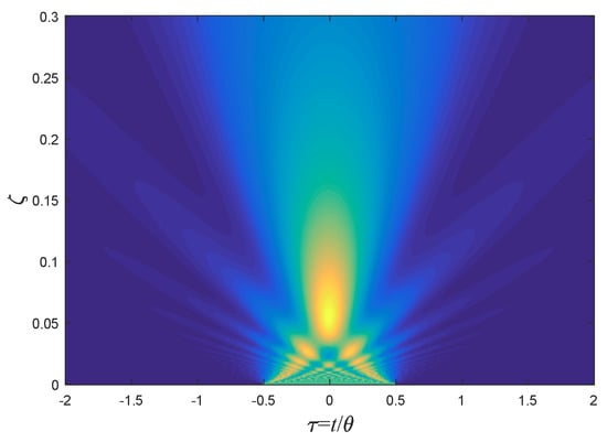
Figure 7.
Same as Figure 2, but for the intensity () of the pulse presented by Equation (27).
The intricate structure of this function is most pronounced when the incident signal is a train of rectangular pulses:
This case is equivalent to the well-known quantum problem of a particle in a 1D box when initially the particle’s probability density is uniform over the box [21].
In this case; the problem’s dynamics can be formulated (using Equation (27)] by
However, it should be emphasized that in Ref. [21] a different numerical approach was taken in which no error function analysis was used.
Sample Application: In 10 Gb/s optical communications channel (over smf28 fiber) with a carrier wavelength of , the pulses can be simulated by rectangular ones with and , in which case in Figure 7 corresponds to . However, as Figure 6 illustrates, considerable distortions appear even for , which corresponds to a fiber length of .
5.3. Chirped Rectangular Pulses
One of the methods to combat dispersion in optical communication is to chirp the pulses, and since most pulses in optical communications are rectangular (in fact they are smooth rectangular, see below) it is instructive to investigate, analytically, the dynamics of a chirped rectangular pulse.
The initial chirped rectangular pulse has the following form:
Therefore, using (10) and (24), the pulse profile after a distance is
Besides the widening of the pulse’s boundaries, the boundaries also move at a constant “velocity”, i.e., the two boundaries obey the following relationship:
Clearly, when is positive, the two boundaries collide at a distance:
which is independent of the pulse’s width . In Figure 8, the propagation of this pulse for both positive and negative is presented.
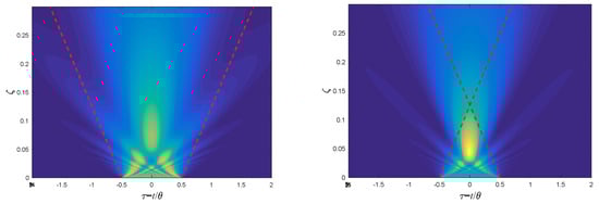
Figure 8.
Same as Figure 2, but for the intensity () of the pulse presented by Equation (31). On the left, ; and on the right, . The dashed lines correspond to the pulse’s boundaries .
While the pulse indeed shrinks for negative , the pulse’s minimum width is reached before the distance , i.e., Equation (33). However, if the two pulses are combined, i.e., if the initial pulse is
then the minimum width occurs exactly at the distance . In Figure 9, the temporal dynamics of this pulse is presented, and the point is clearly shown. Clearly, a smoother, i.e., more realistic, pulse will not converge to an infinitely temporally narrow pulse but instead will converge to a finite temporal width.
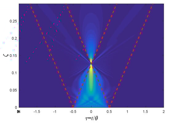
Figure 9.
Same as Figure 8 but with the initial pulse Equation (34) for the parameter .
5.4. Exponential Pulse
The product of the step function with the exponential function allows the investigation of the dynamics of the simplest exponential function. Utilizing Equation (8), the initial exponential-step function
will propagate in a dispersive medium according to
In Figure 10, the dynamics of the exponential-step function pulse is plotted.
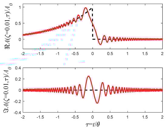
Figure 10.
The real (upper panel) and imaginary (lower panel) components of the exponential-step function pulse (Equation (36)). The dashed curve represents the initial profile (for ), while the solid curve represents its final shape (for ).
A spatiotemporal presentation of the pulse’s intensity is presented in Figure 11. This pulse can simulate a pulse where its rise time is considerably shorter than its decay time. In both Figures, .
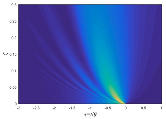
Figure 11.
Same as Figure 2, but for the intensity () of the pulse presented by Equation (36).
5.5. Cosine Pulse
A bounded cosine pulse is an example of a continuous pulse (unlike the rectangular one), where the discontinuity at the edges of the pulse occurs on the amplitude’s derivative level.
It should be stressed that in terms of the pulse’s intensity, the derivative is continuous as well. Therefore, this is an important pulse because, for many practical purposes, it mimics a continuous pulse, but at the same time, it is (initially) temporally bounded.
In this case, if the initial pulse is
which can be rewritten as
then, using Equation (24), the pulse profile at the medium’s end is
Figure 12 illustrates the dynamics of the pulse presented by Equation (39).
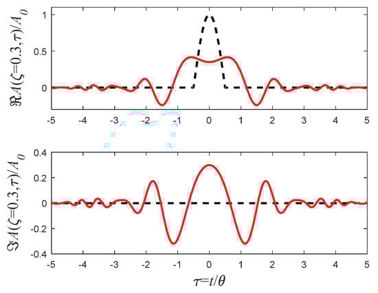
Figure 12.
Similar to Figure 10, but for the bounded cosine pulse (Equation (39)) and for the final distance of .
A spatiotemporal presentation of the pulse’s intensity is presented in Figure 13.
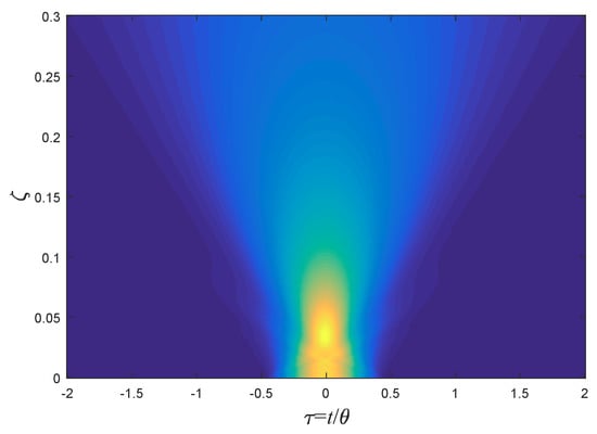
Figure 13.
Same as Figure 2, but for the intensity () of the pulse presented by Equation (39).
5.6. Square Cosine Pulse
A smoother pulse profile is the square cosine one. In this case, the discontinuity occurs in the second derivative level, but the function itself and its derivative are both continuous. Therefore, this pulse can simulate pulses, which were generated by discontinuous dielectric media. Let
be the signal’s profile at one end of the medium; then, since it can be rewritten as
its dynamics can be derived, again using Equation (24), to yield the result at the second end
Figure 14 presents the dynamics of the square cosine pulse.
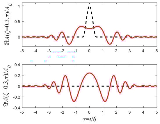
Figure 14.
Similar to Figure 12, but for the square cosine pulse (Equation (42)).
A comparison between Equations (27), (39), and (42) is presented in Figure 15. The three pulses represents three levels of singularities. Equation (27) represents a case of amplitude discontinuity, Equation (39) represents discontinuity in the pulse’s amplitude’s derivative, and Equation (42) represents discontinuity in the amplitude’s second derivative.
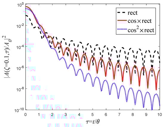
Figure 15.
Comparison between the intensities of the three singular pulses represented by Equation (27)—dashed curve, Equation (39)—solid curve, and Equation (42)—dotted curve in a logarithmic scale.
As can clearly be seen, the higher is the level of the singularity (i.e., the discontinuity occurs at higher derivatives), the faster the pulse decays in accordance with Ref. [22,23].
5.7. Generalization and Applicable Examples
The mathematical tools that were presented in the previous sections can be implemented in numerous practical examples. In what follows we will present some examples.
First example:
Generalization to any power of the bounded cosine pulse, i.e.,
which can be written as
and since the brackets can be expanded
then, using Equation (24), the pulse’s profile at the end of the medium is
Second example:
The initial singular pulse
consists of two exponential pulses, and therefore its propagation can be expressed in a relatively simple form, namely:
Third example:
In the previous example, we sewed two singular pulses; in general, however, one can sew several pulses together to create a combined pulse, which is much smoother than its singular components. For example, take the following pulse profile:
which consist of three singular and discontinuous pulses; however, the combined pulse and its derivative are both continuous. The discontinuity occurs only in the second derivative. In this case the pulse’s amplitude profile obeys
Fourth example:
The discontinuity of the exponential pulse can be reduced by multiplying the pulse by a sine function:
Since the pulse can be written as
then the pulse’s amplitude after a distance z reads
In Figure 16, this pulse is presented for two cases with different parameters. On the right figure, the frequency is equal to the decaying coefficient ; however, on the left figure, the frequency is higher than the decaying exponent , and therefore the profile initially oscillates.
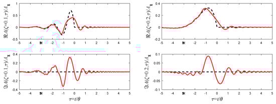
Figure 16.
Similar to Figure 10, but for the pulse presented by Equation (53). In these plots, on both, but on the left figure (final distance corresponds to ) and on the right one (final distance corresponds to ).
6. Smooth Pulses
Thus far, we have analyzed, except for the Gaussian pulses, only singular pulses, i.e., pulse profiles which have at least one singularity point. Most of them can simulate real physical pulse profiles; however, one may argue that these pulses fundamentally cannot behave like physical pulses. In some respects, it is indeed a justified claim, especially for a short medium. It has been shown that since the dispersion equation is not a causal equation, any singularity has nonlocal effects, which do not exist in real pulses [19,20,22,24]. However, it comes out that there is a very elegant method to convert each one of these singular pulses to a smooth one, which can simulate, in all respect, a real physical profile pulse. This method was first presented in Ref. [23,24] for the rectangular pulse.
6.1. Smooth Step Function
In principle, any smooth step function can replace the Heaviside step function; however, there is a clear advantage to choosing the complementary error function for that purpose. The function
is an approximation of the step function in the sense that
However, unlike the step function, the transition in Equation (54) occurs within the time scale .
Equivalently, a step function signal that passes through a Gaussian low-pass filter whose spectral FWHM is will have the following form [11]:
Therefore, the relation between the transition time scale and the spectral FWHM is
Moreover, and this is the reason that Equation (54) is very useful in replacing step functions, the smooth step (Equation (54)) can be written as a convolution between the step function and a Gaussian:
where the asterisk represents temporal convolution. However, since the effect of dispersion can also be represented as a convolution with the kernel (Equation (4)), the propagation of the initial pulse’ profile
can be written simply as
Therefore, every step function from the previous section can be replaced with the smooth step function. In particular, the boosted smooth step function
will have the following profile at the end of the medium:
Sample Applications: The rise time of pulses in optical communications are usually defined as the time period it takes to rise from 10% to 90% maximum intensity value. Therefore, provided this rise-time () is given, can be derived by . If the rise time is defined as the period in which the signal rises from 25% to 75% of its maximum intensity value (), then .
6.2. Smooth Rectangular Pulse
Similarly, the smooth rectangular pulse
will appear at the end of the medium in the following form:
where
is the smooth rectangular function (see Ref. [23,24,25]), which describes the dispersion dynamics of a smooth rectangular pulse.
In Figure 17, this smooth rectangular pulse’s profile is presented for the same values as in Figure 6, i.e., the perfect rectangular pulse. However, the difference is that in Figure 17, the pulse’s boundaries are smooth instead of discontinuous. As can be seen, due to the smooth transition, the oscillations, which appear in Figure 6, disappear in Figure 17.
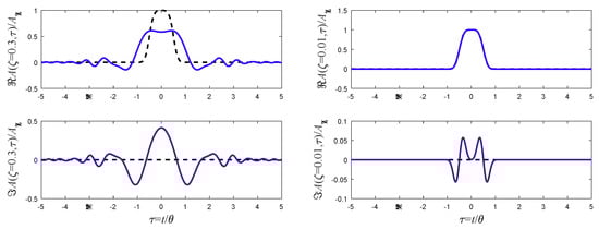
Figure 17.
Same as Figure 12, but for Equation (64) with the transition width .
This pulse has numerous applications in optical communications. For example, if the transmitted data is encoded in the amplitudes of these smooth rectangular pulses, then the transmitted signal profile can be written as
where are coefficients which carry the data.
These pulses have two properties that make them especially suitable for stream of pulses. The parameter can determine the signal’s protocol. The Return-to-Zero (RZ) protocol occurs for , when determines the duty cycle. However, when , then this is a perfect Non-Return-to-Zero (NRZ) protocol. The second property, which is more important, emerges due to symmetry of the erfc function. Since
then two adjacent smooth rectangular pulses look exactly like a single but twice as wide a pulse:
Sample Application: In 40 Gb/s optical communication channels (over smf28 fiber) with a carrier wavelength of , the pulses can be simulated by rectangular ones with , , in which case and in Figure 17 correspond to and , respectively. Since , then the 10–90% rise time corresponds to .
6.3. Relations to Super-Gaussian Pulses
The smooth rectangular pulses can be an excellent approximation for super-Gaussian ones. Let
be a super-Gaussian pulse. This pulse can be approximated by a smooth rectangular one (Equation (63)), , by choosing the following parameters:
and
In Figure 18, such a comparison is presented for two different values of the super-Gaussian order . This figure clearly shows that the smooth rectangular is an excellent approximation to super-Gaussian, while, unlike super-Gaussian, the smooth rectangular pulse does have an exact analytical expression for its propagation in dispersive medium.
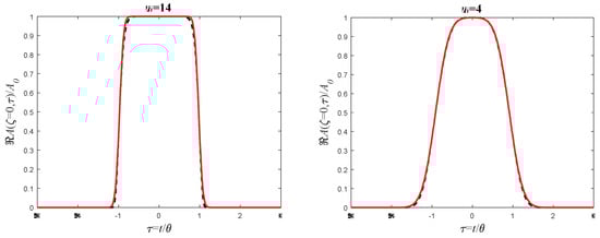
Figure 18.
A comparison between smooth rectangular pulses (Equation (63), solid curves) and super-Gaussian pulses (Equation (69), dashed curves) for (right) and (left). In these plots, only the real part of the fields is presented. The imaginary part is zero.
6.4. Chirped Smooth Rectangular Pulse
The case of the chirped rectangular pulse can be generalized to the chirped smooth rectangular one. That is, if the initial pulse’s profile is
then, after a certain distance in the dispersive medium, the pulse’s profile will be
A spatiotemporal presentation of the pulse’s intensity is presented in Figure 19. The fact that the initial pulse is smooth eliminates the ripples that appear in Figure 8.
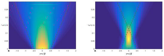
Figure 19.
Same as Figure 8 but for a smooth rectangular pulse with .
6.5. Smooth Cosine Pulse
As was said above, the same procedure can be applied to every singular pulse, i.e., to replace the singular step function with the erfc functions. For example, the singular cosine pulse (Equation (37)) can be replaced with the following smooth cosine one:
which has the following solution for any distance :
Clearly, when , Equation (75) converges to Equation (39). In Figure 20, the amplitude profile of Equation (75) is presented.
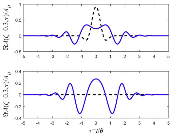
Figure 20.
Same as Figure 12, but for Equation (75) with the transition width .
Clearly, the same procedure can be implemented on the square cosine pulse or on any other singular pulse from the previous sections.
6.6. Smooth Exponential Pulse
By following the same procedure, one can replace the singular exponential with the following smooth exponential pulse:
which propagates in dispersive medium according to
This function is illustrated in Figure 21 for two different distances.
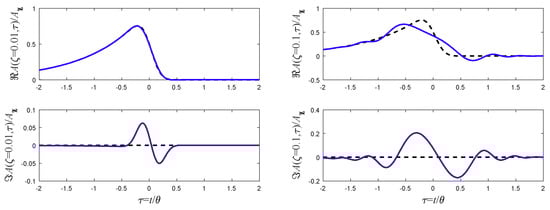
Figure 21.
Same as Figure 10, but for Equation (77) with the transition width and for two final distances on the left and on the right.
Sample Application: A pulse with a 10% to 90% rise time of and a decay time of ~3.7 ps with a carrier wavelength of can be simulated by the pulse presented by Equation (76) with , . Since , Figure 21 is an illustration of this pulse. If the pulse penetrates a BK7 glass, then for this wavelength, , and therefore and in the figure correspond to and , respectively.
7. Singular Pulses in the Spectral Domain
7.1. The ideal Nyquist-Sinc Pulse
One of the interesting and important pulses, which belongs to this category and received a lot of attention recently in the literature, is the Nyquist-Sinc pulse (see, for example, Ref. [26,27,28,29,30,31]).
These pulses are useful in optical communications for several reasons, one of which is that they are resilient against chromatic dispersion. Moreover, these pulses, like their Fourier counterpart, the rectangular pulses, are orthogonal both in the time and in the frequency domains.
The initial Nyquist-Sinc pulse is singular in the spectral domain; its Fourier transform is:
In the temporal regime the “sinc” profile appears:
Since the pulse’s spectrum has a simple rectangular shape, the temporal dynamics is straightforward, namely:
where
is the “dynamic” sinc function [12]. Clearly, .
In Figure 22, the amplitude profile of this pulse is presented.
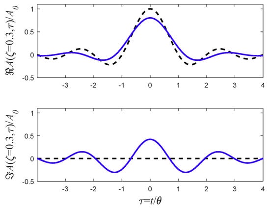
Figure 22.
Same as Figure 10, but for Equation (80) and for the final distance of .
The spatiotemporal presentation of the pulse’s intensity is presented in Figure 23.
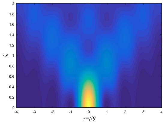
Figure 23.
Same as Figure 2, but for the intensity () of the pulse presented by Equation (80).
7.2. Nyquist Sinc Pulse with Smooth Spectrum
The singular spectrum may simulate real pulses, but in real scenarios, singularities cannot occur even in the spectral domain. We can therefore utilize the theorems and conclusions from the previous sections to spectrally smooth the Nyquist-Sinc pulse.
Thus, the singular rectangular spectrum of the Nyquist-Sinc pulse
can be replaced with its smooth counterpart:
However, this expression can be written as a convolution and is the spectral domain:
and therefore the initial pulse profile can be written as a product of a sinc function and a Gaussian one:
Using Equations (12) and (80), we finally obtain
In Figure 24, the amplitude of Equation (86) is plotted. Unlike ordinary Nyquist-Sinc pulses, this pulse decays exponentially.
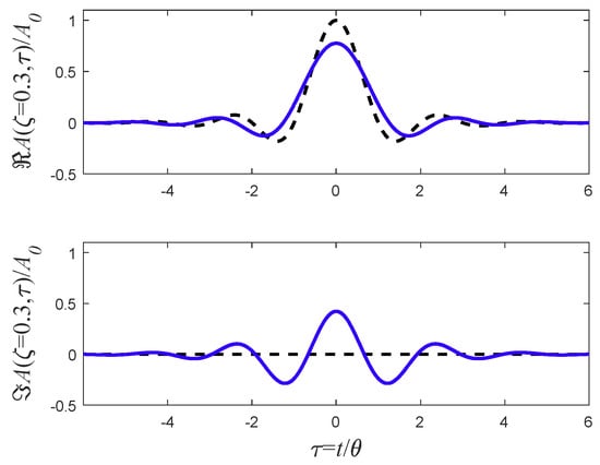
Figure 24.
Same as Figure 22, but for Equation (86) with .
8. Undistorted Airy Pulses
8.1. Undistorted Ideal Accelerating Pulses
One of the interesting properties of the dispersion equation is that the Airy function is its accelerating solution [32,33,34]. However, despite dispersion, the shape of this accelerating solution remains intact during propagation. This property can be useful in optical communications where the encoded data propagates in the dispersive medium without experiencing distortions.
That is, if the initial pulse is an Airy function pulse:
where stands for the Airy function [35], then the pulse at the end of the dispersive medium keeps its initial profile despite being accelerated; after a distance z, it reads:
In Figure 25, the dynamics of this pulse is presented for different distances.
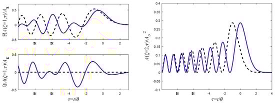
Figure 25.
Presentation of the temporal dynamics of the accelerating Airy pulse (Equation (88)). On the left, the real and imaginary components of the pulse’s field are presented (for the final distance of ), and on the right, the pulse’s intensity () is presented (for the final distance of ).
As can be seen in Figure 25, the pulse’s amplitude shape remains intact, i.e., it keeps the same Airy shape. The only difference is that the pulse’s temporal coordinate [] has shifted with the distance to , and therefore the pulse’s temporal location accelerates according to the equation
Therefore, the square of the dispersion coefficient is proportional to the pulse’s “acceleration”.
8.2. Physical Accelerating Pulse
Clearly, the main problem with the Airy function is that it is not a normalizable function, i.e., it has infinite energy and can have no physical realization.
One option to normalize the airy function is to multiply the pulse by an exponent [36]:
In which case, the pulse dynamics can be derived with the aid of Equations (8) and (88), yielding:
In Figure 26, the dynamics of this pulse is presented. A spatiotemporal presentation of the pulse’s intensity is presented in Figure 27. This pulse has a finite energy (it can be normalized), but as a consequence, the pulse decays in the z-direction as well. Since
the pulse’s confinement within the time-scale “costs” resultant confinement in the z-direction, i.e., the pulse decays within a distance of .
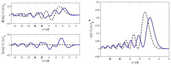
Figure 26.
Same as Figure 25, but for Equation (90) with (for the final distance of ).
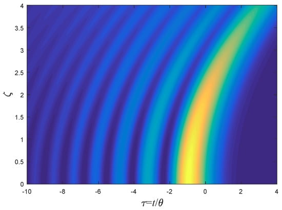
Figure 27.
Same as Figure 2, but for the intensity () of the pulse presented by Equation (92).
8.3. Attenuation Compensating Airy Pulse
It has been realized that the Airy beams can be implemented to compensate medium’s attenuation. Energy can flow from minus infinity to compensate for the pulse’s attenuation. Such a pulse can be constructed by imaginary period displacement [37,38]:
In this case, the pulse at the end of the dispersive medium can be directly derived:
This expression is presented in Figure 28.
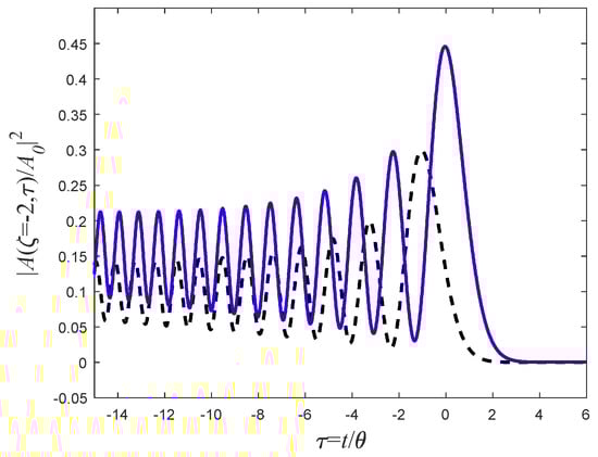
Figure 28.
Same as the right figure in Figure 24, but with .
The introduction of is responsible to the additional exponential term , which can compensate for the medium’s absorption.
The problem with these pulses is, again, that they have infinite energy and cannot be normalized. Therefore, only approximations of these pulses can be implemented in real experiments (see, for example, Ref. [38]).
8.4. Physical Attenuation Compensating Airy Pulse
In the previous section, we have seen that a complex Airy pulse can compensate pulse attenuation. However, these pulses cannot be normalized. One option to turn these pulses to a finite energy ones, and therefore normalizable, is to multiply them by an exponential function, i.e., to choose the following initial pulse profile:
Then, following Equations (8) and (93), the pulse after a distance has the following form:
The intensity of this pulse
is presented in Figure 29 and Figure 30. One can easily see that unlike Figure 25, the pulse’s amplitude increases in short distances, but unlike Figure 28, it has finite energy, and therefore, unlike Equation (94), can be implemented in real physical scenarios.
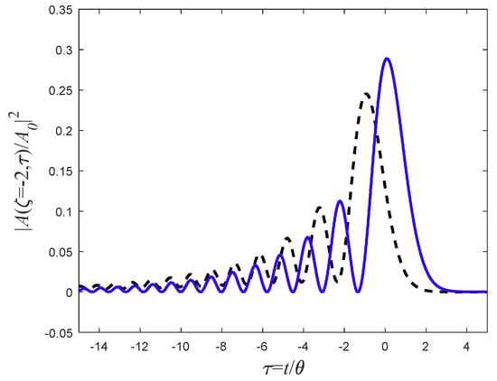
Figure 29.
Same as Figure 28, but for the pulse presented by Equation (97), with and .
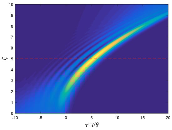
Figure 30.
Same as Figure 2, but for the intensity () of the pulse presented by Equation (97) for and . The horizontal line corresponds for the maximum intensity distance .
Clearly, however, the pulse’s amplitude will eventually decay. It will reach its maximum intensity at , beyond which it will decay to zero. Therefore, this pulse may be implemented to compensate for the medium’s losses when the width of the medium is a given parameter.
9. Pulse Broadening Comparison
To illustrate the large differences between equivalent pulses, the FWHM of four different pulses is presented in Figure 31. To keep the initial FWHM of all pulses equal, the pulses’ parameters were adjusted accordingly. For an arbitrary initial FWHM of T, the FWHM as a function of the normalized distance is presented for Gaussian pulse, i.e., Equation (14) with the parameter ; for smooth rectangular pulse, i.e., Equation (64) with and ; for smooth exponential pulse, i.e., Equation (77) with and ; and finally for Nyquist-Sinc pulse, i.e., Equation (80), with . Clearly, the differences will increase if the signals are chirped.
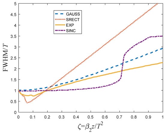
Figure 31.
FWHM Comparison between four different pulses: Gaussian (dashed curve), Rectangular (dotted curve), Exponential (solid curve), and Sinc (dot-dash).
10. Discussion and Conclusions
Dispersive media can have a destructive effect on ultrashort pulses even at relatively short distances.
This paper shows that almost any pulse shape in most practical scenarios can be formulated in a pulse form, whose propagation in dispersive medium has an exact analytical expression.
Therefore, there is no need to restrict the analysis of pulse propagation in a dispersive medium to Gaussian pulses or to numerical analysis. Thus, almost any shape and form of pulses can be analyzed analytically. This is the main result and main conclusion of this paper.
The experimentalist can choose from the multiple examples presented in this paper to predict the distortions that the relevant pulse would experience.
In particular, if the pulses were generated by a mode-locked laser, then a Gaussian pulse is a good approximation. However, if there is an asymmetry between the pulse’s rise and fall times (as in Q-switch lasers), then the experimentalist can use the smooth exponential pulses (Section 6.6) to predict the pulse’s distortions.
Similarly, in modern optical communications channels, the data signals consist of multiple pulses which mostly belong to two categories: rectangular and Nyquist pulses. Both types of pulses are presented in this paper; however, these pulses are both discontinuous: The former is discontinuous in the time domain while the latter is discontinuous in the frequency domain. In practical cases, the signals are always continuous (in both time and frequency domains). Therefore, the experimentalist or the engineer can measure the pulse’s rise time and apply the smooth rectangular pulses (Section 6.2) to the relevant system to predict the pulse’s distortion in the fiber. Similarly, Nyquist-Sinc pulses with a smooth spectrum (Section 7.2) can be used to simulate real systems, which are based on Nyquist-Sinc pulses. The exact dispersion’s distortion can be evaluated without the need for approximations or for numerical analysis.
Moreover, this paper demonstrates that any singular pulse can be replaced with a smooth pulse whose evolution in dispersive medium can be formulated in an exact analytical form.
Besides this generic recipe, the main new findings are the exact analytical derivations of the following pulses: (A) chirped rectangular pulses, which converge to extremely narrow pulses; (B) excellent analytical approximation of super-Gaussian pulses; (C) Nyquist-Sinc Pulses with a smooth spectrum; and (D) a physical realization of attenuation-compensating Airy pulses.
Funding
This research received no external funding.
Conflicts of Interest
The author declares no conflict of interest.
Appendix A. Proof of Equation (3)
The spectral transfer function of the medium is
i.e., for the incident signal the signal after a distance of z is simply . In general, let be the Fourier transform of then
Since the Fourier transform of a product is a convolution of the Fourier transforms, then the application of the Fourier transform on Equation (A2) yields
where
is the Fourier transform of .
Appendix B. Proof of Equation (6)
Let
and let us further assume that
is given. Then
which, after some calculations, can be rewritten as
Using Equations (A6) and (A4), Equation (A8) is simply
Appendix C. Proof of Equation (10)
Let
and let us further assume that
is given. Then
Which, after some algebra, can be written as
Using Equation (A11), Equation (A13) can simply be rewritten as
References
- Zevallos, M.E.; Gayen, S.K.; Das, B.B.; Alrubaiee, M.; Alfano, R.R. Picosecond Electronic Time-Gated Imaging of Bones in Tissues. IEEE J. Sel. Top. Quantum Electron. 1999, 5, 916–922. [Google Scholar] [CrossRef]
- Gayen, S.K.; Alfano, R.R. Emerging optical biomedical imaging techniques. Opt. Photon. News 1996, 7, 17–22. [Google Scholar] [CrossRef]
- Das, B.B.; Yoo, K.M.; Alfano, R.R. Ultrafast time-gated imaging in thick tissues: A step toward optical mammography. Opt. Lett. 1993, 18, 1092–1094. [Google Scholar] [CrossRef] [PubMed]
- Marom, D.M.; Sun, P.C.; Fainman, Y. Communication with ultrashort pulses and parallel-to-serial and serial-to-parallel converters. In Proceedings of the LEOS ‘97, 10th Annual Meeting IEEE Lasers and Electro-Optics Society, San Francisco, CA, USA, 10–13 November 1997. [Google Scholar]
- Amiri, I.S.; Ahmad, H. Optical Soliton Communication Using Ultra-Short Pulses; Springer: Singapore, 2015. [Google Scholar]
- Yamaoka, Y.; Harada, Y.; Sakakura, M.; Minamikawa, T.; Nishino, S.; Maehara, S.; Hamano, S.; Tanaka, H.; Takamatsu, T. Photoacoustic microscopy using ultrashort pulses with two different pulse durations. Opt. Express 2014, 22, 17063–17072. [Google Scholar] [CrossRef] [PubMed]
- Gibbs, H.C.; Arne, Y.B.; Alvin, C.L.; Yeh, T. Imaging embryonic development with ultrashort pulse microscopy. Opt. Eng. 2014, 53, 051506. [Google Scholar] [CrossRef]
- Technical Note: The Effect of Dispersion on Ultrashort Pulses. Newport Corporation (2018). Available online: https://www.newport.com/n/the-effect-of-dispersion-on-ultrashort-pulses (accessed on 10 January 2018).
- Sindhu, T.G.; Bisht, P.B.; Rajesh, R.J.; Satyanarayana, M.V. Effect of higher order nonlinear dispersion on ultrashort pulse evolution in a fiber laser. Microw. Opt. Technol. Lett. 2001, 28, 196–198. [Google Scholar] [CrossRef]
- Wang, W.; Liu, Y.; Xi, P.; Ren, Q. Origin and effect of high-order dispersion in ultrashort pulse multiphoton microscopy in the 10 fs regime. Appl. Opt. 2010, 49, 6703–6709. [Google Scholar] [CrossRef] [PubMed]
- Granot, E. Fundamental dispersion limit for spectrally bounded On-Off-Keying communication channels and its implications to Quantum Mechanics and the Paraxial Approximation. Europhys. Lett. 2012, 100, 44004. [Google Scholar] [CrossRef]
- Granot, E. Information Loss in Quantum Dynamics. In Advanced Technologies of Quantum Key Distribution; INTECH: Rijeka, Croatia, 2017. [Google Scholar]
- Wollenhaupt, M.; Assion, A.; Baumert, T. Femtosecond Laser Pulses: Linear Properties, Manipulation, Generation and Measurement. Chap. 12. In Hanbookd of Laser and Optics; Träger, F., Ed.; Springer: New York, NY, USA, 2007. [Google Scholar]
- Agrawal, G.P. Fiber-Optic Communications Systems, 3rd ed.; John Wiley & Sons, Inc.: New York, NY, USA, 2002. [Google Scholar]
- Crank, J. The Mathematics of Diffusion; Clarendon Press: Oxford, UK, 1975. [Google Scholar]
- Ali, R.; Hamza, M.Y. Propagation behavior of super-Gaussian pulse in dispersive and nonlinear regimes of optical communication systems. In Proceedings of the International Conference on Emerging Technologies (ICET 2016), Islamabad, Pakistan, 18–19 October 2016. [Google Scholar]
- Anderson, D.; Lisak, M. Propagation characteristics of frequency-chirped super-Gaussian optical pulses. Opt. Lett. 1986, 11, 569–571. [Google Scholar] [CrossRef]
- Zhang, L.; Li, C.; Zhong, H.; Xu, C.; Lei, D.; Li, Y.; Fan, D. Propagation dynamics of super-Gaussian beams in fractional Schrödinger equation: From linear to nonlinear regimes. Opt. Express 2016, 24, 14406–14418. [Google Scholar] [CrossRef]
- Moshinsky, M. Diffraction in time. Phys. Rev. 1952, 88, 625–631. [Google Scholar] [CrossRef]
- Del Campo, A.; Garcia-Calderon, G.; Muga, J.G. Quantum Transients. Phys. Rep. 2009, 476, 1–50. [Google Scholar] [CrossRef]
- Berry, M.V. Quantum fractals in boxes. J. Phys. A Math. Gen. 1996, 29, 6617–6629. [Google Scholar] [CrossRef]
- Granot, E.; Marchewka, A. Generic Short-Time Propagation of Sharp-Boundaries Wave Packets. Europhys. Lett. 2005, 72, 341–347. [Google Scholar] [CrossRef]
- Granot, E.; Luz, E.; Marchewka, A. Generic pattern formation of sharp-boundaries pulses propagation in dispersive media. J. Opt. Soc. Am. B 2012, 29, 763–768. [Google Scholar] [CrossRef]
- Granot, E.; Marchewka, A. Emergence of currents as a transient quantum effect in nonequilibrium systems. Phys. Rev. A 2011, 84, 032110–032115. [Google Scholar] [CrossRef]
- Marciano, S.; Ben-Ezra, S.; Granot, E. Eavesdropping and Network Analyzing Using Network Dispersion. Appl. Phys. Res. 2015, 7, 27. [Google Scholar] [CrossRef]
- Soto, M.A.; Alem, M.; Shoaie, M.A.; Vedadi, A.; Brès, C.-S.; Thévenaz, L.; Schneider, T. Optical sinc-shaped Nyquist pulses of exceptional quality. Nat. Commun. 2013, 4, 2898. [Google Scholar] [CrossRef]
- Schmogrow, R.; Bouziane, R.; Meyer, M.; Milder, P.A.; Schindler, P.C.; Killey, R.I.; Bayvel, P.; Koos, C.; Freude, W.; Leuthold, J. Real-time OFDM or Nyquist pulse generation—Which performs better with limited resources? Opt. Express 2012, 20, B543. [Google Scholar] [CrossRef]
- Hirooka, T.; Ruan, P.; Guan, P.; Nakazawa, M. Highly dispersion-tolerant 160 Gbaud optical Nyquist pulse TDM transmission over 525 km. Opt. Express 2012, 20, 15001–15007. [Google Scholar] [CrossRef]
- Hirooka, T.; Nakazawa, M. Linear and nonlinear propagation of optical Nyquist pulses in fibers. Opt. Express 2012, 20, 19836–19849. [Google Scholar] [CrossRef] [PubMed]
- Schmogrow, R.; Hillerkuss, D.; Wolf, S.; Bäuerle, B.; Winter, M.; Kleinow, P.; Nebendahl, B.; Dippon, T.; Schindler, P.C.; Koos, C.; et al. 512QAM Nyquist sinc-pulse transmission at 54 Gbit/s in an optical bandwidth of 3 GHz. Opt. Express 2012, 20, 6439–6447. [Google Scholar] [CrossRef] [PubMed]
- Bosco, G.; Carena, A.; Curri, V.; Poggiolini, P.; Forghieri, F. Performance limits of Nyquist-WDM and CO-OFDM in high-speed PM-QPSK systems. IEEE Phot. Technol. Lett. 2010, 22, 1129–1131. [Google Scholar] [CrossRef]
- Berry, M.V.; Balázs, N.L. Nonspreading wave packets. Am. J. Phys. 1979, 47, 264–267. [Google Scholar] [CrossRef]
- Siviloglou, G.A.; Broky, J.; Dogariu, A.; Christodoulides, D.N. Observation of Accelerating Airy Beams. Phys. Rev. Lett. 2007, 99, 213901. [Google Scholar] [CrossRef] [PubMed]
- Bandres, M.A. Accelerating beams. Opt. Lett. 2009, 34, 3791–3793. [Google Scholar] [CrossRef]
- Abramowitz, M.; Stegun, A. Handbook of Mathematical Functions; Dover Publications: New York, NY, USA, 1965. [Google Scholar]
- Siviloglou, G.A.; Christodoulides, D.N. Accelerating finite energy Airy beams. Opt. Lett. 2007, 32, 979. [Google Scholar] [CrossRef] [PubMed]
- Preciado, M.A.; Dholakia, K.; Mazilu, M. Generation of attenuation-compensating Airy beams. Opt. Lett. 2014, 39, 4950–4953. [Google Scholar] [CrossRef]
- Preciado, M.A.; Sugden, K. Proposal and design of airy-based rocket pulses for invariant propagation in lossy dispersive media. Opt. Lett. 2012, 37, 4970–4972. [Google Scholar] [CrossRef]
© 2019 by the author. Licensee MDPI, Basel, Switzerland. This article is an open access article distributed under the terms and conditions of the Creative Commons Attribution (CC BY) license (http://creativecommons.org/licenses/by/4.0/).