Effective Crack Damage Detection Using Multilayer Sparse Feature Representation and Incremental Extreme Learning Machine

Abstract

Detecting cracks within reinforced concrete is still a challenging problem, owing to the complex disturbances from the background noise. In this work, we advocate a new concrete crack damage detection model, based upon multilayer sparse feature representation and an incremental extreme learning machine (ELM), which has both favorable feature learning and classification capabilities. Specifically, by cropping and using a sliding window operation and image rotation, a large number of crack and non-crack patches are obtained from the collected concrete images. With the existing image patches, the defect region features can be quickly calculated by the multilayer sparse ELM autoencoder networks. Then, the online incremental ELM classified network is used to recognize the crack defect features. Unlike the commonly-used deep learning-based methods, the presented ELM-based crack detection model can be trained efficiently without tediously fine-tuning the entire-network parameters. Moreover, according to the ELM theory, the proposed crack detector works universally for defect feature extraction and detection. In the experiments, when compared with other recently developed crack detectors, the proposed concrete crack detection model can offer outstanding training efficiency and favorable crack detecting accuracy.

1. Introduction

Concrete structures play a predominant role in civil construction. Owing to internal and external factors, crack damage will inevitably occur in concrete structures, and crack defects are the main reasons for the reduction of bearing capacity, durability, and waterproofing of concrete structures. Therefore, studying the detection methods of concrete crack damage is of great importance for the safety assessment of concrete structures, the prediction of service life, and the resistance of natural disasters.

Researchers have presented many methods to detect concrete cracks. The readers can refer to one review article [1], which discussed the current practices and emerging techniques for pavement distress detection. For the crack damage areas, the pixel value is distinct from those of the background contents, and could be seen as a demarcation line of the concrete image. As a result, several crack damage detecting methods using global analysis have been presented. Abdel et al. applied four edge detectors for finding the concrete cracks, and a fast Haar transform was identified as the best solution [2]. In [3], curvelet transform is utilized for detecting the void diseases in ballast-less track, which may result in the cracks of the track slab. Hutchinson developed one Canny edge-based crack detection, which utilized a semi-automatic threshold value [4]. With the operation of empirical mode decomposition, a Sobel operator was applied for detecting the crack regions in [5]. However, only fifteen simple images were used in their experimental results, which is not suitable for the complexity of typical backgrounds. Cho et al. also presented one inspection method for concrete surface cracks using terrestrial laser scanning [6]. In [7], image preprocessing (transforms, filters, edge detector, and so on) was applied for addressing the background noises, and then the crack areas were detected by a decision tree. In addition, similar to the edge-based crack detection methods, an Otsu based algorithm was exploited for segmenting the crack regions from the backgrounds [8]. Based on the Canny detecting results, Wang et al. applied the K-means algorithm for exploring the crack regions [9]. Chatterjee et al. utilized one adaptive threshold strategy for preliminary crack segmentation, which can remove most of the background content [10]. However, in practice, the gray scales of an identical crack region may vary widely, in terms of non-uniform illuminations or other background disturbances, and perhaps the corresponding crack detecting results were bad.

To solve the problem, the local analysis based crack detection model is proposed. Generally, by dividing the raw image, many image patches can be first obtained. Then, the two-class classifier is applied for determining the crack regions. Usually, the crack detection methods by local analysis are made up of two parts—a feature extracting process and crack damage region identification. Through the contribution of advantageous feature presentation and a powerful classification technique, the local analysis-based crack detectors have achieved better performances than the general crack detectors based on global analysis. Recently, many works have used different region feature presentations or feature classification techniques.

For the image region feature representation, the mean value and variance value of image patches were calculated by Oliveira [11]. Similarly, the moment feature extraction was utilized for detecting the crack regions in [12]. These region features, mentioned above, are simple and easily affected by background shadows. For coping with this illumination challenge, Chen et al. exploited the local binary patterns (LBP) model for extracting the region features of concrete images [13]. Additionally, the histogram features of image patches were computed in [14], which can improve the crack detecting performances.

In the case of the fine concrete structure environment, the hand-crafted feature representations above can acquire the discriminating image region feature sets. However, due to the complicated background changes, the artificially designed features may not well depict the cracks and backgrounds, which becomes one of the limiting factors of crack detecting performance. For instance, the LBP descriptor calculates the texture features of image region. Although the LBP model can perform well with the illumination challenge, it is unable to deal with unknown background noises. Therefore, it is preferable to learn a feature representation from the existing image data, rather than predefining a generic feature extraction model.

After the image region feature extraction, the followed crack damage detecting process is designed to build one feature classification model. Specifically, the constructed feature classifier is utilized for recognizing the cracks among all the candidate image regions. Recently, some representative crack region classification algorithms have been advocated; Jahanshahi et al. applied a SVM model for determining the optimal identification function between the crack images and non-crack ones [15]. Bu et al., calculated the wavelet region features of concrete images, and then presented one bridge crack detecting method, based on SVM techniques [16]. In order to explore multitudinous crack damages, one binary-tree network using a SVM method has been proposed in [13]. An artificial neural network (ANN) is a computing framework, inspired by biological learning, which has been applied in fatigue life prediction [17], surface inspection [18], and in many other areas. In [19], the back propagation (BP) based neural network classification method has been presented for detecting possible crack regions. As the training performance of the BP method is very slow, a varying slope of the activation function is advocated for training the crack region recognition model [20]. Additionally, the ensemble learning method can be also used for crack region identification. In [21], Wang et al. combined multi-scale random decision forests and the wavelet transform for detecting potential crack regions.

The above-mentioned crack region detecting models have obtained some satisfactory detecting results. However, the SVM-based crack detectors need to solve a quadratic programming problem and the ANN-based crack detectors are confronted with tedious iterative parameter tuning. Generally speaking, one concrete image should be separated into many small regions. Thus, for these crack region detection methods (including ensemble learning), the numerous image patches will involve a high computational burden. More importantly, considering the emergence of new crack and non-crack instances, it is necessary to update the crack region detector incrementally. However, these existing crack region classifications do not take into consideration this problem.

Recently, deep learning (DL) models have gained significant attention, due to their successes in learning feature representation and classification, and thus, were also applied for surface defect detection [22,23], face identification [24], crack damage detection, and so on. Through experimental results in [25], the convolutional neural network (CNN)-based crack detector has been proved to be better than the edge-based one. Zhang and Yang et al. applied the multi-layer CNN technique for extracting crack damage features, and the fullly connected neural network is used as the final classification layer [26]. Cha et al. identified the crack and no-crack patches by training one CNN model with a sliding window technique, which obtained much better performances than the traditional edge-based detections [27]. Chen et al. combined the CNN model and a native Bayes data fusion strategy for detecting crack regions [28], and achieved superior performance, compared with their original LBP-based crack detection method [13]. Xu et al. exploited multi-layer restricted Boltzmann machines (RBMs) for learning the abstract features of an input image, and reported satisfactory detecting results in their experiments [29].

Generally, deep learning based crack damage feature extracting often contributes to better detecting performances than the traditional hand-crafted features. However, these methods have several parameters that must be iteratively fine-tuned. Therefore, most of the existing DL-based crack detecting frameworks face the slow learning problem, which may hinder their practical use in real-time detecting applications. Moreover, as for the DL-based crack detecting architecture, both the multi-layer feature learning networks and the following binary classification network are “hard coded” together. Thus, we have to retrain the whole neural network when dealing with new training samples, which is a time consuming task and not appropriate for sustainable crack damage detection.

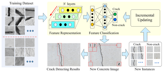
As seen from the above analysis, we found that a good crack damage detector should have several characteristics: (1) Feature representation should be discriminative enough for the background disturbances, while being processed efficiently. (2) Crack region identification should have a low computing burden and can be quickly updated incrementally. (3) Considering that there may be some background disturbances (e.g., handwriting, etc.) similar to cracks, how to minimize the relevance between cracks and those noises is an important quality of robust crack detection. In this work, we only place emphasis on the first two points, and present a new crack damage detecting model by using the excellent feature learning and classification capabilities of an extreme learning machine (ELM).

Unlike the greedy, layer-wise training in general DL-based crack detection, the presented crack detection consists of two separate parts: Unsupervised multilayer crack region feature extracting and supervised crack region identification. For the first part, a sparse ELM-based auto-encoder (AE) is used for extracting the multi-layer sparse features of the input images; while for the second part, we derived the incrementally updated crack feature classification model using online sequential ELM. The main advantage of developed crack detection is that it has a faster training efficiency than the deep learning methodologies, while keeping a good performance at the same time.

It should be mentioned that, although the ELM theories have been well established, our work focuses on developing an effective and efficient crack detector. To our knowledge, this is the first time the ELM theories have been used to construct a comprehensive framework, including feature extraction and crack region identification, for a concrete crack damage detecting application. The contributions are summed, as follows.

(1) We propose an effective multilayer feature representation for learning the image features of crack or non-crack images. Unlike existing unsupervised feature learning strategies (i.e., BP-based NNs) for crack detection, an efficient ELM auto-encoder is used to build the hierarchical feature learning pipeline. Owing to its randomly-chosen input hidden parameters, the presented image region feature learning network can be quickly built. Moreover, to further enhance learning of informative features, a sparsity constraint for the ELM-AE output weights is imposed, and an accelerated proximal gradient (APG) algorithm is utilized for processing the feature learning task.

(2) An efficient crack region binary classification has been developed. Compared with traditional learning algorithms (SVM or neural networks), the proposed feature classification network is free from the BP-based iterative parameter tuning and, thus, the corresponding final crack region detector can be efficiently calculated. Furthermore, we have derived the incremental updating expression of the presented crack region identification model, which can be trained with the chunk-by-chunk available training samples.

The rest of this work is detailed as follows. As the presented crack detector was developed based on ELM, the ELM details are briefly reviewed in Section 2. Section 3 shows the details of the presented crack damage detecting model, involving the multi-layer feature representation and the incrementally updated crack feature classification. Experimental results are shown and discussed in Section 4. In Section 5, the final conclusions are given.

2. ELM Contents

To help in understanding the presented crack detecting algorithm, we briefly review the theory and concepts of ELM, as follows. For more detailed contents, the readers can refer to these works [30,31,32,33].

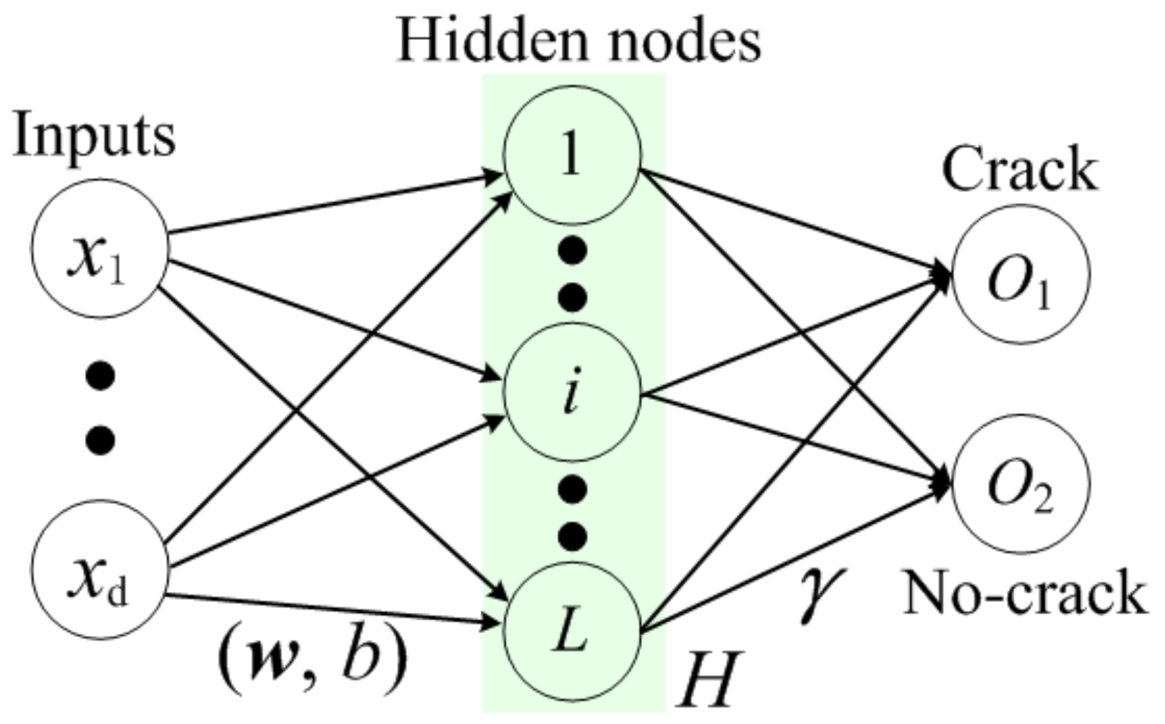
The ELM was initially proposed for studying the single hidden layer feedforward neural network (SLFN) [30]. As shown in Figure 1, with L hidden nodes (here, L is an important parameter for ELM model), a SLFN can be expressed as

$$f_L\left(x\right)={\sum }_{i=1}^{L}G\left({\mathit{w}}_i,b_i,x\right){\mathit{\gamma }}_i={\sum }_{i=1}^L{h}_i\left(x\right){\mathit{\gamma }}_i,$$

(1)

where x is the input data of ELM network, $b_i$ represents the bias of i-th hidden node, ${\mathit{w}}_i$ denotes the input weight linking the inputs x and the i-th hidden node, $G(·)$ is the variant sigmoid function, $h_i(·)$ denotes the output vector of i-th hidden node, and $\mathit{\gamma }$ is the ELM network output weight, which needs to be computed.

Differing from other neural network frameworks, the ELM model shows that the hidden input parameters (i.e., $b_i$ and ${\mathit{w}}_i$ in the $G\left({\mathit{w}}_i,b_i,x\right)$ function) can be randomly chosen from a continuous probability distribution [30]. Thus, the ELM framework can obtain a much faster training performance than other learning models. Moreover, Huang et al. have proven that ELM has both universal approximation capability and classification capability:

Theorem 1.

Universal approximation capability [31]: Given any bounded nonconstant piecewise continuous function as the activation function, if the SLFNs can approximate any target function $f\left(x\right)$ via tuning the parameters of hidden neurons, then the sequence ${\left\{h_i\left(x\right)\right\}}_{i=1}^L$ could be randomly generated based on any continuous sampling distribution, and ${lim}_{L\to \infty }∥{\sum }_{i=1}^L{h}_i\left(x\right){\mathit{\gamma }}_i-f\left(x\right)∥=0$ holds with probability 1 with appropriate output weight γ.

Theorem 2.

Classification capability [32]: Given any feature mapping $h\left(x\right)$, if $h\left(x\right)\mathit{\gamma }$ is dense in $C\left({\mathbb{R}}^d\right)$ or in $C\left(M\right)$, where M is a compact set of ${\mathbb{R}}^d$, then SLFNs with random hidden layer mapping $h\left(x\right)$ can separate arbitrary disjoint regions of any shapes in ${\mathbb{R}}^d$ or M.

For simplicity, we can rewrite Equation (1) as $f_L\left(x\right)={\sum }_{i=1}^L{h}_i\left(x\right){\mathit{\gamma }}_i=\mathbf{H}\left(x\right)\mathit{\gamma }$. Here, $\mathbf{H}\left(x\right)=\left[h_1\left(x\right),\dots ,h_L\left(x\right)\right]$ represents the row outputs of ELM network. If we randomly generate the input hidden parameters, $\mathbf{H}\left(x\right)$ will be known and, then, the ELM learning function will be linear. In this case, finding the output weights $\mathit{\gamma }$ becomes the only objective goal. Suppose that the training sets are $\left\{\mathbf{X},\mathbf{T}\right\}={\left\{x^i,t_i\right\}}_{i=1}^N$. Here, $x^i\in {\mathbb{R}}^d$ denotes the i-th input data and $t_i\in {\mathbb{R}}^m$ is the corresponding training label. The linear learning function can be expressed in the following matrix form

$$\mathbf{H}\mathit{\gamma }=\mathbf{T},$$

(2)

where $\mathbf{H}$ represents the randomized matrix of ELM hidden layer, and can be computed as follows:

$$\mathbf{H}=\left[\begin{array}{c}h\left(x^1\right)\\ ⋮\\ h\left(x^N\right)\end{array}\right]=\left[\begin{array}{ccc}{h}_1\left(x^1\right)& \cdots & h_L\left(x^1\right)\\ ⋮& \ddots & ⋮\\ h_1\left(x^N\right)& \cdots & h_L\left(x^N\right)\end{array}\right].$$

(3)

Based upon the ELM learning theory [33], the training process of an ELM network needs to achieve both the smallest training error and the smallest norm of $\mathit{\gamma }$:

$$\widehat{\mathit{\gamma }}=\underset{\mathit{\gamma }}{argmin}\left\{{∥\mathit{\gamma }∥}_2^2+\lambda {∥\mathbf{T}-\mathbf{H}\mathit{\gamma }∥}_2^2\right\}.$$

(4)

According to the theorems above, ELM learning framework has obtained satisfactory performances in many applications; for example, fault diagnosis [34], face recognition [35], power prediction [36], fatigue stress estimating [37], and so on. Inspired by these, in this work, we try to utilize ELM for effective and efficient performance of the crack damage detection task.

3. Proposed Crack Detection Model

3.1. Overall Framework

In this work, a new crack damage detection model is proposed; the overall framework is shown in Figure 2. It can be seen that this framework is made up of two phases: (1) Multi-layer image region feature representation and (2) incremental crack region classification.

Before the feature learning phase, many representative crack and non-crack image patches are generated by partitioning the collected concrete images, which are used for constructing the training data set. In the feature learning process, a fast ELM-based auto-encoder is utilized for extracting the hidden sparse features of the input images. Based on the created single layer feature learning network, N-layer unsupervised feature learning is performed to calculate the high level sparse crack features of the input images. Then, with the computed multilayer region features, an efficient crack region classification model is advocated, using the ELM classified network.

When dealing with a new test image, we first divide it into non-overlapping image patches, and then the trained crack damage detector is utilized for finding these crack damage patches. With the rough crack detection results, morphological image processing is used to combine the disconnected cracks and eliminate the isolated background blocks. After processing several concrete images, some fresh non-crack and crack training examples are obtained for incrementally updating the advocated crack detection model.

3.2. Multilayer Feature Representation

Owing to the limited performances of hand-crafted features, most of the existing concrete crack detection methods are unable to achieve satisfactory results under the condition of complicated surroundings. Meanwhile, the DL-based feature learning models need expert knowledge, and require time-consuming parameter fine-tuning. To address the problems mentioned above, we present an efficient multi-layer feature learning scheme, based on an ELM-based auto-encoder (AE).

An AE is usually utilized for unsupervised feature learning. In an auto-encoder, the input $x\in {\mathbb{R}}^d$ is mapped into a latent representation $\psi \in {\mathbb{R}}^{L_f}$, and the resulting $\psi$ is used to recover the input x via minimizing the reconstruction errors. Here, $L_f$ is an important parameter of AE, and its value setting will be discussed later. Differing from the traditional auto-encoders, ELM-AE randomly projects the inputs x by a non-linear function $h\left(x\right)=G(\mathbf{w},\mathbf{b},\mathbf{X})$, and searches the way to recover the original data x by $h\left(x\right)\mathit{\gamma }=x$. As $h\left(x\right)$ is given, ELM-AE can learn the image features faster than the existing methods (e.g., deep Boltzmann machine), and has achieved favorable performance in image classification [38].

The success of ELM-AE feature representation has inspired us to extend it to crack region feature extraction. The proposed single layer feature learning model mainly consists of two steps: ELM feature training and ELM-AE feature mapping. Suppose that, in an ELM-AE with $L_f$ hidden nodes, the input data set is $\mathbf{X}=\left\{{\mathbf{x}}_{\mathbf{1}},{\mathbf{x}}_{\mathbf{2}},\dots ,{\mathbf{x}}_{\mathbf{N}}\right\}$, where $x_i\in {\mathbb{R}}^d$ is the i-th input vectorizing the image region data. As mentioned above, we randomly choose the hidden parameters $\mathit{w}$ and b (see Equation (1)), which project the input data $x_i\in {\mathbb{R}}^d$ into an $L_f$ dimensional ELM random space, as follows:

$$H_i={\left\{G({\mathit{w}}_j,b_j,x_i)\right\}}_{j=1}^{L_f},i=1,\dots ,N.$$

(5)

For ELM feature training, the main objective is to reconstruct the inputs $\mathbf{X}$ from ELM random space H by solving the following problem:

$$\widehat{\mathit{\gamma }}=\underset{\mathit{\gamma }}{\mathrm{argmin}}\left\{{∥\mathbf{X}-\mathbf{H}\mathit{\gamma }∥}_2^2+\mu {∥\mathit{\gamma }∥}_p\right\},$$

(6)

where $\mathit{\gamma }$ is the output weight to be obtained and $\mu$ is a regularization parameter. The setting of p controls the characteristics of the ELM learning. To obtain more sparse and meaningful hidden features, we set p to be the ${\ell }_1$ norm.

To efficiently solve Equation (6), a fast APG algorithm [39] is adopted for getting the optimum result within several iterations. The APG method can attain an $O\left(1/\phantom{1k^2}{k}^2\right)$ convergence rate with k iterations. In this case, the object function of Equation (6) can be rewritten as

$$\left\{\begin{array}{c}f\left(\mathit{\gamma }\right)={∥\mathbf{X}-H\mathit{\gamma }∥}_2^2\hfill \\ g\left(\mathit{\gamma }\right)=\mu {∥\mathit{\gamma }∥}_1\hfill \end{array}\right.$$

(7)

where $f\left(\mathit{\gamma }\right)$ is a differentiable smooth convex function with Lipschitz continuous gradient and $g\left(\mathit{\gamma }\right)$ is a non-smooth but convex function. The gradient of the smooth convex function is $\nabla f\left(\mathit{\gamma }\right)=2H^{\mathrm{T}}\left(H\mathit{\gamma }-\mathbf{X}\right)$, and its corresponding Lipschitz constant is $\xi =2\times max\left(eig(H·H^{\mathrm{T}})\right)$. The details for finding the output weight $\mathit{\gamma }$ can be found in Algorithm 1.

Algorithm 1: The ELM feature training process.

Input: The image data $\mathbf{X}$, number of hidden nodes $L_f$,      Lipschitz constant $\xi$, regularization parameter $\mu$.   1: Begin the iteration by taking ${\mathit{\gamma }}_0={\mathit{\gamma }}_{-1}=\mathbf{0}\in \mathbb{R}{}^{L_f\times d}$; and setting $t_0=t_{-1}=1$ as the initial value.   2: Compute the following equations, $k=0,1,2\cdots$ $\left\{\begin{array}{c}{V}_k={\mathit{\gamma }}_k+\frac{t_{k-1}-1}{t_k}\left({\mathit{\gamma }}_k-{\mathit{\gamma }}_{k-1}\right)\hfill \\ M=V_k-\nabla f\left(V_k\right)/\phantom{\nabla f\left(V_k\right)\xi }\xi \hfill \\ {\mathit{\gamma }}_{k+1}=\mathrm{sgn}\left(M\right)·max\left(0,\left|M\right|-\mu /\phantom{\mu \xi }\xi \right)\hfill \\ t_{k+1}=\left(1+\sqrt{1+4t_k^2}\right)/\phantom{\left(1+\sqrt{1+4t_k^2}\right)2}2\hfill \end{array}\right.$   Output: The optimal output weight $\widehat{\mathit{\gamma }}$.

By solving Equation (6), we can obtain the optimal output weight $\mathit{\gamma }$. As described in [38], $\mathit{\gamma }$ can account for the input image region data using singular values, and can be treated as the learned image basis for describing the input data distributions.

In this subsection, one validation experiment was carried out. As illustrated in Figure 3, 10,000 crack region images were used as the inputs of a single layer ELM-AE feature learning network, whose hidden node number was $L_f$. Here, the hidden node number $L_f$ was an important parameter, and its setting and effects on crack detection performance will be discussed in Section 4.4. Using Algorithm 1, the optimal output weight $\mathit{\gamma }\in {\mathbb{R}}^{L_f\times d}$ can be calculated, and each row data of $\mathit{\gamma }$ is squeezed to a $d_1\times d_1$ ($d=d_1^2$) matrix image data. The generated matrix image set is illustrated in Figure 3b, and one can see that they contain the input crack region distributions (see red ellipse in Figure 3b). Therefore, similar to the coding strategy in dictionary feature learning [40], the product of the inputs x and learned basis $\mathit{\gamma }$ can provide a compact feature representation, y, of the inputs:

$$y=J(x·\mathit{\gamma }),$$

(8)

where $J(·)$ denotes a non-linear sigmoid function. Based on the presented single layer ELM-based feature learning model, a multi-layer feature learning scheme can be easily performed to obtain the high level sparse region features of input concrete image patches. Specifically, the output weight of the previous layer is utilized as the inputs of the current one, and the output weights of each hidden-layer network are independently computed by layer-wise unsupervised computing. The learned image region features of k-th layer network are as follows:

$$y_k=F_1({\mathbf{H}}_k,{\mathit{\gamma }}_k;y_{k-1}),$$

(9)

where ${\mathbf{H}}_k$ is the generated randomized matrix of k-th layer network, ${\mathit{\gamma }}_k$ is the desired k-th layer ELM-AE output weight, $F_1(·)$ is the ELM-based feature learning model, and $y_k$ is the k-th layer learned image region feature to be calculated. As previously stated, the output of N-th layer unsupervised learning is calculated as the inputs of the supervised ELM-based classification network, thereby achieving the final crack region detecting function.

3.3. Incremental Crack Region Classification

In this section, as for the crack region detection, we utilize a regularized ELM-based classification model, and its stability and generalization performance have been studied, in particular, in [32].

Specifically, suppose that the hidden-node number of ELM classifier is $L_c$, and we randomly generate the input-hidden parameters ${\mathbf{w}}_j$ and $b_j$ ($j=1,\cdots ,L_c$). Here, $L_c$ is an important parameter for ELM-based classification network, and its value will be discussed later. With these generated hidden parameters, the hidden layer matrix can be easily computed via $H_i={\left\{h_j\left(y_i\right)\right\}}_{j=1}^{L_c}$$(i=1,\dots ,N)$. Here, $h_j\left(y\right)=G(w_j,b_j,y)$ denotes the j-th hidden-node output of ELM network and $y_i$ represents the i-th learned image region feature. The training process of crack region classification needs to solve the following problem [41]:

$$\begin{array}{c}\underset{\mathit{\beta }}{min}\frac{1}{2}{∥\mathit{\beta }∥}^2+\frac{\lambda }{2}\sum _{i=1}^N{∥e_i∥}^2\hfill \\ \mathrm{s}.\mathrm{t}.h\left(y_i\right)\mathit{\beta }=t_i-e_i,i=1,\cdots ,N,\hfill \end{array}$$

(10)

where $\mathit{\beta }$ denotes the required output weights of the ELM classifier, $t_i$ is the training label of inputs $y_i$, and $\lambda$ is the regularized parameter for penalizing the training error term $e_i$. By substituting the constraints into the objective function, For Equation (10), solving the following problem is equivalent:

$$\underset{\mathit{\beta }}{min}\frac{1}{2}{∥\mathit{\beta }∥}^2+\frac{\lambda }{2}{∥H\mathit{\beta }-T∥}^2.$$

(11)

For solving the problem Equation (11), the gradient, with respect to $\mathit{\beta }$, can easily be calculated. The optimal solution ${\mathit{\beta }}^{*}$ can then be obtained by setting this gradient function to be 0.

$${\mathit{\beta }}^{*}=(I/\phantom{(I\lambda }\lambda +H^{\mathrm{T}}H{)}^{-1}{H}^{\mathrm{T}}T,$$

(12)

where $\mathbf{I}$ represents an identity matrix whose dimension is the hidden node number $L_c$ of ELM classification model. The required crack damage identification decision function, $F_2(·)$, is

$$F_2\left(y\right)=\mathbf{H}\left(y\right)·{\mathit{\beta }}^{*}.$$

(13)

Along with the continuous concrete crack damage detecting tasks, some new non-crack and crack concrete images will be available. To adapt to the changing concrete surroundings, it is necessary to renew the old crack damage detection network. As is known to us, retraining the initial ELM classification model using the old and new training samples is a straightforward way. Despite the fact that this motivation is simple, it will be faced with the burden of storage and computation time with an increasing number of training data.

In this section, for solving this problem above, the online incremental updating method is adopted for updating the advocated crack damage identification network. It should be mentioned that the randomly generated hidden parameters (i.e., ${\mathbf{w}}_j$ and $b_j$) will be not changed in the ELM network retraining. In this case, the output weight $\mathit{\beta }$ of ELM network becomes the only option parameter to be updated.

If we already have $Z_0$ training sample features, including crack and non-crack image patches, the primeval ELM hidden output matrix ${\mathbf{H}}_0$ can be easily calculated, and the corresponding training labels are ${\mathbf{T}}_0$. According to Equation (12), the initial crack damage identification function can be computed, as follows:

$${\mathit{\beta }}_0=(I/\phantom{(I\lambda }\lambda +H_0^{\mathrm{T}}{H}_0{)}^{-1}{H}_0^{\mathrm{T}}{T}_0.$$

(14)

For simplicity, we rewrite $P_0=I/\phantom{P_0=I\lambda }\lambda +H_0^{\mathrm{T}}{H}_0$, and $Q_0=H_0^{\mathrm{T}}{T}_0$. Then, we have ${\mathit{\beta }}_0={\mathbf{P}}_0^{-1}{\mathbf{Q}}_0$.

Now, there are $Z_1$ new training sample features, and ${\mathbf{T}}_1$ corresponds to the training output labels. Then, the hidden layer output matrix ${\mathbf{H}}_1$ can be computed easily, and the output weight matrix of crack damage identification network is updated, as follows:

$${\mathit{\beta }}_1=P_1^{-1}{Q}_1.$$

(15)

Specifically, considering the new training data and the old training ones, we get

$$\begin{array}{c}{P}_1=I/\phantom{I\lambda }\lambda +{\left[H_0,H_1\right]}^{\mathrm{T}}\left[H_0,H_1\right]\hfill \\ =I/\phantom{I\lambda }\lambda +H_0^{\mathrm{T}}{H}_0+H_1^{\mathrm{T}}{H}_1\hfill \\ =P_0+H_1^{\mathrm{T}}{H}_1,\mathrm{and}\hfill \end{array}$$

(16)

$$\begin{array}{c}{Q}_1={\left[H_0,H_1\right]}^{\mathrm{T}}\left[T_0,T_1\right]\hfill \\ =H_0^{\mathrm{T}}{T}_0+H_1^{\mathrm{T}}{T}_1=Q_0+H_1^{\mathrm{T}}{T}_1\hfill \\ =P_0{\mathit{\beta }}_0+H_1^{\mathrm{T}}{T}_1.\hfill \end{array}$$

(17)

Substitute Equation (16) into Equation (17), we have

$$Q_1=P_1{\mathit{\beta }}_0-H_1^{\mathrm{T}}{H}_1{\mathit{\beta }}_0+H_1^{\mathrm{T}}{T}_1.$$

(18)

Finally, by combining Equations (18) and (15), we get the incremental updating equation

$${\mathit{\beta }}_1={\mathit{\beta }}_0+P_1^{-1}\left(H_1^{\mathrm{T}}{T}_1-H_1^{\mathrm{T}}{H}_1{\mathit{\beta }}_0\right).$$

(19)

Based on the derivation results above, we can see that the proposed online incremental retraining function only needs to compute the new data, and can obtain the same learning performances as the simple training process with the total training samples (including new and old training data). Thanks to this, it is our opinion that the presented updated method is suitable for the practical concrete crack damage detecting task.

4. Experiments and Discussion

4.1. Experimental Settings

To verify the effectiveness and efficiency of our work, four representative crack damage detection methods are compared with the proposed model. Specifically, these compared methods are the Otsu based crack- [8], the Canny based- [4], the SVM based- [11], and the DL based-crack detectors [26]. Among them, the first two models belong to the global analysis based crack detection model, and the latter two are categorized as the crack detection method by local analysis. What we should note, here, is that these compared crack damage detecting algorithms were programmed by ourselves, based on their original methods.

For fairness, the presented crack detector, and all the compared ones, are programmed on the same computer (Win7 x64 system, Matlab2017b, Intel 2.40GHz CPU, 64GB RAM, GTX960 GPU). As for the local analysis based methods (including the presented method and the latter two compared ones [11,26]), the same training samples and testing concrete image data were used.

4.2. Database Generation

For evaluating the presented crack defect detecting method, in this work, 400 concrete images with a resolution of $4608\times 3456$ pixels were practically collected using a Canon HS125 camera. These concrete images were obtained from several concrete structures (e.g., deck slab, beams, and so on) at Shijiazhuang Tiedao University, China.

In addition, to achieve the best performance of our proposed model, some guidelines for image acquisition are suggested here (but are not required): (1) Images should have sufficient resolution so that objects and cracks can be seen. (2) Perspective angle between the camera and concrete structure should not be large. With a larger perspective angle, the crack regions may be occluded by other objects. (3) Distance between the camera and concrete structure should keep roughly constant. If the distance becomes larger, the crack object will be very tiny, and may be omitted by the complicated surroundings. If the distance is very small, the width of cracks will be very large, and only the edge of cracks may be detected by the presented method.

As for the training and cross-validation of the crack damage detector, we randomly choose 300 images from the total 400 concrete images. In order to ensure the complexity of training data, these images should contain various conditions (e.g., non-uniform illumination, shadows, blurring, pockmark, attachment, crack-like, and so on). The effectiveness of the proposed approach was tested on the remaining 100 images, which were not used for the training and validation processes.

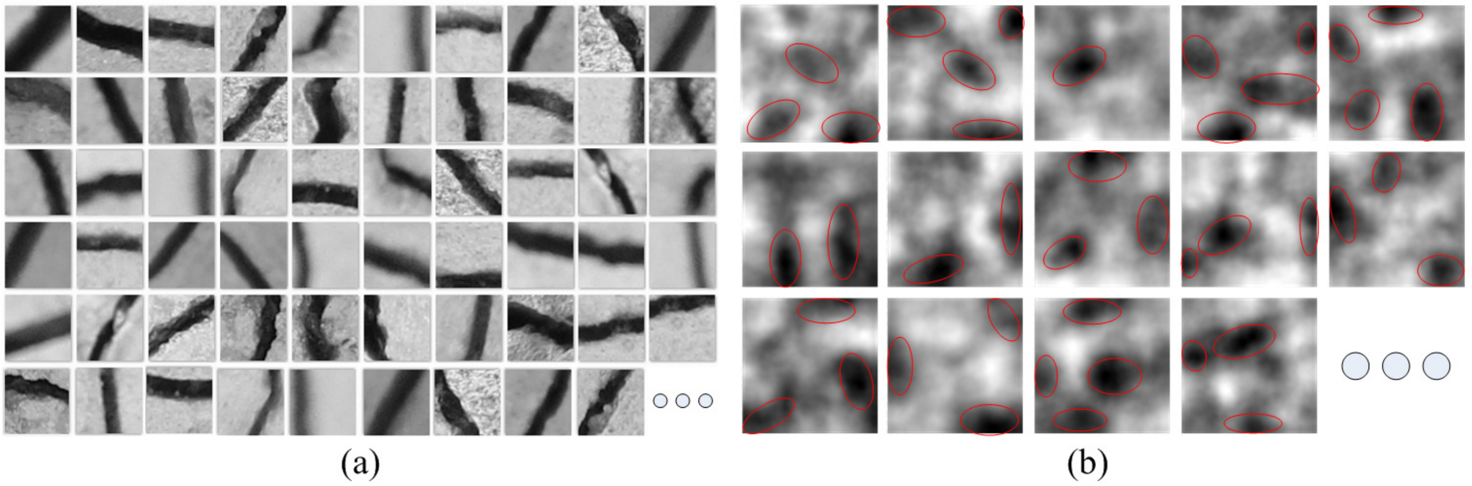
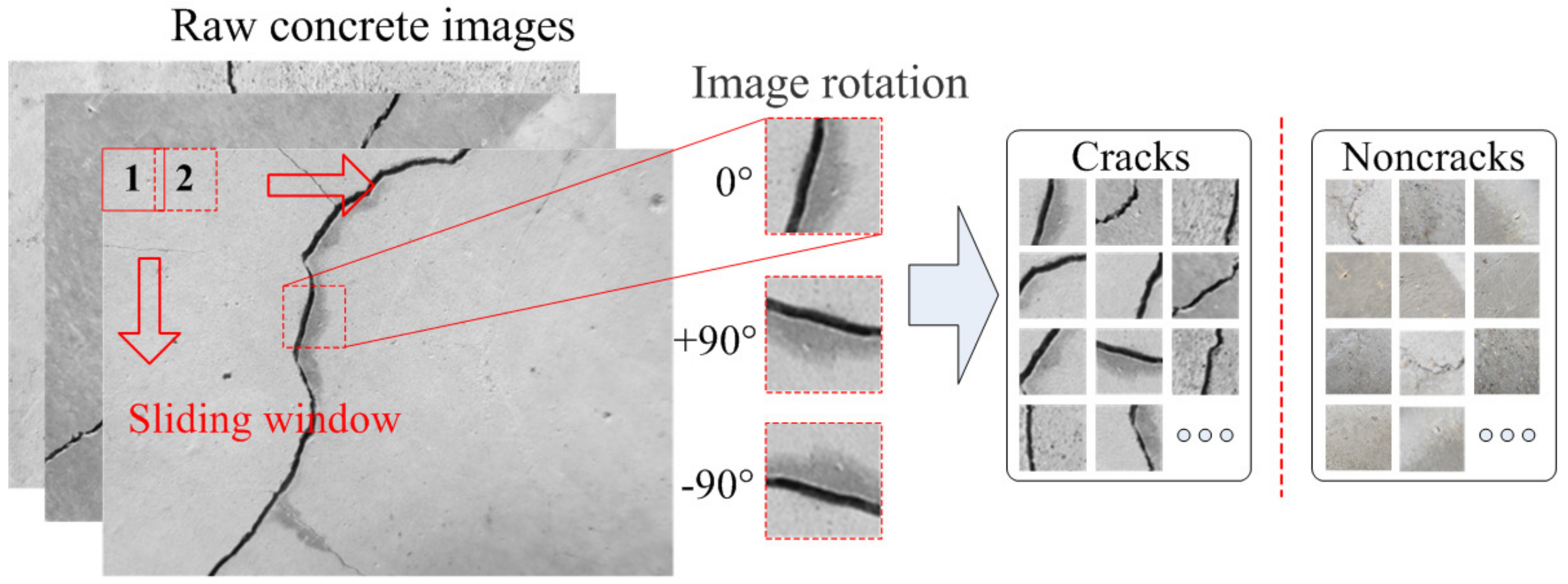
In this work, for training the ELM-based crack detector, large amounts of small image patches of $n\times n$ pixels are required. By dividing these 300 training images in an overlapped manner, plenty of candidate training samples were generated. With help of manual operation, the typical image regions, including crack or non-crack samples, were collected. As shown in Figure 4, for obtaining more patterns of crack or non-crack images, the partitioned image patches were rotated by −90 degrees and 90 degrees. Finally, the total number of prepared training image samples was 50,000, which contained 25,000 non-crack samples and 25,000 crack ones.

For training process, we randomly selected ninety percent of the crack samples and ninety percent of the non-crack ones. The rest of the training image samples were utilized for cross-validation testing process. In this paper, for one well-trained ELM-based crack detector, the training accuracy and cross-validation testing accuracy should be larger than 0.9.

As for the testing process, each one of these remaining 100 images was divided into non-overlapped image patches of $n\times n$ pixels. Then, the advocated ELM-based crack detection model was employed for finding the crack regions among all the separated candidate ones. By artificially labeling these divided candidates, the testing accuracy (i.e., false negative rate or false positive rate) could be computed, which can be used to evaluate the performance of presented method quantitatively.

4.3. Selection of Image Patch Size

The element size of the image patches plays an important role in detecting crack damages. In principle, if the patch size is very small, the small image region may occupy the inside of the crack object, thereby leading to less detection accuracy. If the patch size is very large, there may be other background disturbances (e.g., attachments) involved in the crack training samples. In this case, the discrimination between crack samples and background ones will be decreased, which will affect the classification performance of the presented method. For selecting a suitable image patch size, a series of patch size $n\times n$ (n = 30, 45, 75, 100, 125) were chosen as inputs for training the ELM-based detecting network. The specific training process is as follows: First of all, the $n\times n$ image patch was stretched into one $1\times n^2$ data vector, which was used as the input layers after normalization. The following two-layer ELM-AE network, consisting of $L_f$ and $L_f$ hidden units, was trained with randomly generated hidden parameters. The presented Algorithm 1 was utilized for training the ELM-AE sparse network to obtain the optimal output weights. Then, for separating the cracks from backgrounds, one binary ELM classification network, with $L_c$ hidden nodes, was employed as the output layer. Finally, the presented ELM-based detecting network architecture was $n^2-L_f-L_f-L_c-2$, and each layer in the stack architecture was trained independently. Using the same amount of training samples and the same training parameters mentioned above, the training accuracy and cross-validation testing accuracy have been plotted in Figure 5. It can be seen that the training accuracy reached the maximum value (97.1%) when the n was 75, and the validation accuracy (96.7%) was also the largest for this element size. Therefore, for obtaining a good detecting ratio of crack damage, the size parameter of divided image patches was set to be $75\times 75$ pixels.

4.4. Parameter Selection

Compared with DL-based crack detecting methods [26,27,29], there were only a few parameters to be adjusted in the training steps of presented crack detector. As introduced in Section 3, there are mainly three user specified parameters to be adjusted. Specifically, they are the hidden node number $L_f$ of the ELM-AE feature representation, the hidden node number $L_c$ of the ELM feature classification, and the regularization parameter $\lambda$ of the ELM classification model.

In our work, as for multi-layer feature learning process, the hidden node number of each layer was set to be the same, which is similar to the preferred setting of [38]. Technically, there is no good way of choosing these parameter values above. In this paper, they were to be chosen by the trial and error method. Figure 6 illustrates the 3D testing accuracy and training time plots using different parameters. Note that the testing accuracy result was calculated using the testing image patches, which are from the 50,000 image data set.

As depicted in Figure 6a,c, one can see that the parameter $\lambda$ plays a vital role in the testing accuracy of the proposed crack detector. Mathematically, $\lambda$ regulates a balance between the smallest training error and the norm of the ELM output weights. As $\lambda$ decreases, the accuracy of crack region detection is correspondingly reduced. It should also be mentioned that different $\lambda$ values have similar training time (see Figure 6b,d), and so do not affect the training efficiency of our work.

Moreover, in Figure 6a,c, it can be seen that the performance of presented method degrades rapidly from ${log}_{10}\left(\lambda \right)$ = 0 to ${log}_{10}\left(\lambda \right)$ = −5. The reason for this result may be that, compared with the norm of the ELM output weights, the training error item is more important for the training process. Therefore, the generalization of the crack detector becomes very bad when there is less emphasis on the training error item.

For setting the hidden node number of the ELM network, from the Figure 6a,c, the performances of our model are mainly very stable within the wide scope of $L_f$ and $L_c$ with a large parameter $\lambda$. The hidden node number value represents the Vapnik-Chervonenkis dimension of the ELM network. With a larger hidden number, there will be more nodes to be calculated in the feature learning or classification, and the resultant training time is obviously increased (see Figure 6b,d). On the other hand, the crack damage detecting method would have a poor discriminative capability with too small of a hidden node number. In this case, the trained function cannot separate the crack patches from those background ones in the testing process. From Figure 6a,c, one can see that a larger hidden node number contributes to the testing accuracy, especially when $\lambda$ is small.

Additionally, as shown in Figure 6a, there is also a harsh slope between $L_f$ = 1000 and $L_f$ = 500 when $\lambda$ is small. The possible reason for this is that the learned ELM-AE features becomes more compact when the $L_f$ value is smaller than 1000. In this case, the discrimination between crack features and non-crack ones will be decreased, thereby leading to the performance degradation of proposed method.

Based on the analyses mentioned above, the setting of the $\lambda$ value has no effect on the training efficiency. Therefore, in the point of view of detection accuracy, $\lambda$ was set to be a larger value (i.e., ${10}^9$). For setting the values of $L_f$ and $L_c$, the crack classification performance was given priority, and the computational burden can be reduced by some efficient computing platforms (e.g., graphic processing units). With this consideration, $L_f$ in the ELM feature representation was set to be 2000, and $L_c$ in the ELM classification was set to be 6000.

4.5. Qualitative Evaluation

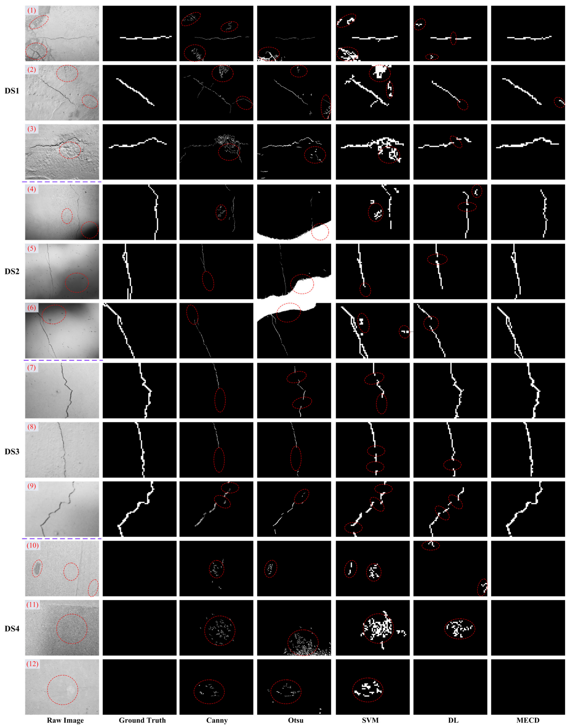
In this subsection, some representative crack region detection results are shown in Figure 7. Specifically, the 100 concrete test images were divided into three types: Dataset 1, which contained cracks and background disturbances; Dataset 2, which had cracks and illumination changes; and Dataset 3, which contained cracks and image blurring. Moreover, some additional concrete images constituted Dataset 4, which contained some background noises but did not involve any crack damage region. For simplicity, these testing datasets, mentioned above, are named DS1, DS2, DS3, and DS4, respectively. For better comparison, the ground truth of each concrete image is shown in the second column of the figure. The right-hand five columns show the crack damage detecting results of Canny [4], Otsu [8], SVM [11], DL [26], and the advocated multilayer ELM-based crack detector (named to be the MECD model), respectively. The specific performance discussions are as follows.

(1)

Background Disturbances

For dealing with the images from DS1, one can see whether the crack detection methods can tackle the disturbances in a complex environment (e.g., pockmark, attachment, or crack-like). As for the Canny-based method, some tiny background noises can be filtered using the Gaussian image filtering process. There are still several blocky background mistakes (see Figure 7(1–2)), however, and, as their areas and visual parameters are unknown, it is impossible to remove them by using naive post-processing methods. The Otsu-based method can perform clustering-based image segmentation automatically. However, in some cases, the pixel gray values of local concrete image regions are close to those of crack defects. For instance, in Figure 7(1), the attachments nearby the true crack damages are easily mistaken using the Otsu based model. The post-morphological processing can delete some mistaken background noises, but these visual parameters of mistaken identified areas are indeterminate and, thus, the resultant crack detection results were not satisfactory.

From the illustrations in Figure 7(3), it can be seen that stripes are easily mistaken for crack damages, using the SVM-based method. A possible reason may be that it only adopts naive image region features and, consequently, the subsequent SVM classification model cannot obtain a robust hyperplane between crack samples and non-crack ones. For the DL based crack damage detection model, thank to the strong feature learning capabilities of the multi-layer network, the attachment or pockmark disturbances (see Figure 7(2–3)) can be well addressed. However, the whole crack regions may not be recognized by a DL-based crack detector. For instance, in Figure 7(3), the in-between regions of crack objects are mistakenly identified as non-cracks. A possible reason is that the visual features of the undetected crack areas are close to those of some of the background troubles (e.g., the stripes shown in Figure 7(1)). However, the discrimination between the ambiguous potential crack regions and background disturbances is not good enough in the DL-based crack detector.

From the compared performances above, it is clear that the presented MECD model has obtained satisfactory detecting results, reasoning by the following two points: (1) The developed multi-layer sparse feature representation can extract the high-level region features of image patches—compared with the existing DL-based crack detection model, ELM theory has already proved that the random feature projection can satisfy the universal approximation capability [31], and, thus, more important contents of crack image regions can be extracted for hidden-layer feature learning, which can well deal with complicated background noises. (2) An accurate ELM-based crack region identification model was exploited for the ultimate pattern decision of image patches. With ELM theory [31], high-dimensional non-linear mappings of obtained high-level features can offer a satisfactory feature classification precision.

(2)

Illumination Changes

Figure 7 further presents some crack region detecting results with illumination challenges. For the Canny-based model, the gaussian filtering technique can alleviate the troubles of random surrounding disturbances. However, with the global image smoothing operation, some local little cracks may be left undetected (see Figure 7(5–6)). Besides, the Canny-based model may not deal with large-area surrounding troubles (e.g., the background noises of Figure 7(4)), which cannot be deleted using the naive edge based algorithms. Due to non-uniform illuminations, it is possible that there are multiple histogram peak values for one single concrete image. In this case, the Otsu-based crack detection model was unable to determine the optimal segmentation threshold, and performed badly. Additionally, the falsely segmented local image regions were connected with the true crack damage areas, and could not be well addressed by naive post-processing methods.

For addressing the concrete images from DS2, by contrast, the SVM-based crack detector can obtain preferable detection results, and could almost identify all of the crack areas through local image region binary classification. However, there were still some background false alarms (i.e., the red ellipse dashed boxes in Figure 7), which may have been due to its adopted simple statistical image region features. Unlike SVM based methods, the DL-based crack detection method utilized multilayer convolutional neural networks for computing the high level image region features, which could deal with the surrounding noises well. However, owing to the curse of the local minima issue during the greedy layer-wise training, it is impossible that the DL-based crack detector could recognize the total crack regions (see Figure 7(4–6)).

(3)

Image Blurring

Due to the movement or exposure issues when collecting the concrete images, there may be image blurring or degradation, which may bring about difficulty in recognizing the true crack damage areas. Simply put, the boundary line of the crack region may be unclear, due to the image blurring problem. With this condition, the crack damage detecting models using edge analysis (e.g., Otsu and Canny) failed to detect the whole crack damage regions using the blurry concrete image, as depicted in Figure 7(7–9). Compared with the SVM based crack detector, DL and our presented MECD method performed better for coping with the image blur problem. However, the curved parts of blurry images were not well recognized by the DL-based method (see Figure 7(9)). By comparison, the presented method exploited the multi-layer ELM-based sparse feature representation, which could extract the compact and sparse hidden information of input image patches. With the resulting informative image region features, and the followed ELM based crack classification process, the developed crack damage detecting model achieved more accurate detecting results.

4.6. Field Demonstration

In this subsection, to verify the performance of presented crack detection model, field demonstration has been carried out. As shown in Figure 8a, the developed crack detector was utilized for finding the surface crack damage regions of a concrete beam, which was undergoing a fatigue experiment using a fatigue machine at Shijiazhuang Tiedao University, China. Obviously, it can be seen that there were many difficult background disturbances in the field demonstration. For example, Figure 8b,c show the two sides of concrete beam, which had iron chains, surface-mounted cable, reinforcement, illumination changes, painting markers, and so on. Figure 8d depicts the crack damages from the concrete bridge deck, and there was litter on the bridge deck. Figure 8e–i illustrate some stress-concentration areas of the concrete beam, and there were some cracks appearing in these areas. One can see that there were three-colored painting markers on the concrete surface (white, black, and red). From the experimental results, we can see that the proposed method addressed most of the background disturbances. It should be noted that there was one limitation for the advocated crack detection method. As shown in the dashed ellipses of Figure 8e, the black painted line was not correctly identified by our presented method. A possible reason is that, compared with other color painting markers, the black painted lines were more similar to the true cracks.

4.7. Crack Region Detecting Accuracy

In this subsection, the crack region detecting accuracies of the proposed method and of the other compared crack detectors are discussed. First of all, six kinds of divided image patches from the 100 test concrete images were calculated: P (positive) is the number of image patches containing cracks; N (negative) denotes the number of image patches excluding cracks; $FN$ (False Negative) denotes the number of crack regions which were identified as non-cracks; $FP$ (false positive) denotes the number of non-crack regions which were identified as cracks; $TP$ (true positive) represents the number of correctly detected to be crack regions; and $TN$ (true negative) denotes the number of correctly detected non-crack regions. The crack region detecting accuracy of a crack detector was computed with the $FNR$ (false negative rate) and $FPR$ (false positive rate) criteria, as follows:

$$\begin{array}{c}\hfill \left\{\begin{array}{c}FNR=\frac{FN}{P}\times 100\%\hfill \\ FPR=\frac{FP}{TP+FP}\times 100\%.\hfill \end{array}\right.\end{array}$$

(20)

It should be noted that the two criteria, mentioned above, require the accurate number of cropped image patches. In this case, the Otsu and Canny crack detections can not be valued. Using the three testing Datasets (i.e., DS1, DS2, and DS3) containing cracks, the experimental results of the local analysis-based crack detectors (i.e., DL, SVM, and the presented MECD model) are shown in

Table 1. Comparisons of crack region testing accuracy. SVM; Support Vector Machine.

Challenges	DataSets (Number)	Method	P	N	TP	TN	FN	FP	FNR (%)	FPR (%)
Background disturbances	DS1 (59)	SVM	24,780	140,774	23,797	138,271	983	2503	3.97%	9.52%
		DL			23,107	140,049	1673	725	6.75%	3.04%
		MECD			24,328	140,262	452	512	1.83%	2.06%
Illumination changes	DS2 (31)	SVM	14,260	72,726	13,637	70,710	623	2016	4.37%	12.88%
		DL			13,348	72,268	912	458	6.40%	3.32%
		MECD			13,962	72,411	298	315	2.09%	2.21%
Image blurring	DS3 (10)	SVM	2800	25,260	2584	24,871	216	389	7.71%	13.08%
		DL			2444	25,164	356	96	12.71%	3.78%
		MECD			2718	25,204	82	56	2.93%	2.02%
Average testing accuracy	DS1,DS2,DS3 (100)	SVM	41,840	238,760	40,018	233,852	1822	4908	4.35%	10.92%
		DL			38,899	237,481	2941	1279	7.03%	3.18%
		MECD			41,008	237,877	832	883	1.99%	2.11%

.

Mathematically, the $FNR$ value represents the ratio between the mistakenly identified crack patches and the manually labeled crack patches. It is obvious that a crack detection model with a small $FNR$ value would have a high crack damage detecting performance. As shown in Table 1, one can see that the presented MECD model achieved the best detecting results (with a $FNR$ value lower than $0.03$) among all the compared crack detectors. Similarly, the $FPR$ value denotes the ratio between the falsely recognized non-crack patches and the total number of detected crack regions, which depicts the incorrect detection rate of crack regions. Generally, a favorable crack detector should have a small $FPR$ value. From the comparisons of Table 1, the developed MECD method has achieved the most satisfactory result, with a $FPR$ value within the bounds of 0.025.

Through the comparisons, it is clear that the proposed MECD method and DL-based method have smaller $FPR$ values than SVM-based one. A possible reason is that the MECD model and DL-based one both exploit multi-layer crack region feature representation, thereby addressing the troublesome surrounding noises will. Furthermore, the DL-based crack defect detection had a larger $FNR$ value than our developed MECD algorithm, which may be due to the over-fitting issue.

4.8. Comparison in Training Efficiency

As mentioned in Section 4.2, for improving crack damage detecting performances, plenty of training image patches were generated by an overlapping partitioned operation. The generated mass training image samples brought about a heavy computational load for obtaining the crack detector. In this work, we place emphasis on developing an effective and efficient crack detector. One novelty of our developed algorithm is the successful application of ELM in the multilayer crack region feature learning and classification. Compared with other learning frameworks (SVM or neural networks), the MECD model can obtain better generalization results with an efficient training speed, which will contribute to the application of proposed crack damage detection method. As these edge-based crack detection methods do not require the training step, only the crack detectors using local binary classification are discussed in this subsection. Specifically, the presented MECD method, the SVM-based one [11], and the DL-based one [26] are compared, in the aspect of training efficiency.

Table 2. Training time and software environment of the crack damage detecting model.

Method	SVM1	SVM2	DL	MECD1	MECD2
Training time (second)	243.6	34.6	1025	88.3	27.6
Implementation	MATLAB + C	MATLAB + GPU	MATLAB + GPU	MATLAB	MATLAB + GPU

shows the training time of the compared crack detection methods, using the same amount of training samples. In addition, the software environment also has an effect on the training time of crack detector. In this paper, though all the compared models apply the MATLAB program, there are still several distinctions for implementing the crack defect detecting task. Here, the specific programming settings are shown at the bottom side of Table 2.

As for the comparisons, with the utilization of the fast C-mex function, the SVM-based method can alleviate the high computational burden of the quadratic programming process. However, the SVM technique is a shallow classification model, and its corresponding result was not advantageous when compared with the multi-layer neural networks (i.e., DL and MECD). Among these compared models, the DL-based method applied the deep BP-based neural network for the image feature learning process and, thus, the total training process became very slow. For improving the calculating efficiency, the graphic processing unit (GPU) option was utilized. Despite all this, the DL-based method was still the most inefficient training method. By contrast, the MECD method was more efficient than DL-based one, which is due to the following two points: (1) The adopted ELM-AE feature learning could be quickly implemented with the APG method. (2) The ELM feature classification network did not need to be fine-tuned. Therefore, due to the two reasons above, the presented MECD model tended to achieve faster training performances than DL-based method.

Moreover, for fair comparison, we attempt to implement the three crack detectors in the same software environment (MATLAB + GPU). Specifically, for the SVM-based crack detector, cuSVM toolbox [42] was utilized for the binary SVM training task, and the corresponding training time was about 7 times faster (see Table 2) than that of implementation using the C-mex function. In addition, as for the proposed MECD model, the ELM classification was performed using the ELM-GPU toolbox [43], and the resultant training time was about 3 times faster (see Table 2) than that of the original MECD model. Through further comparison, one can see that the proposed MECD method was still the most efficient crack detecting model, and the corresponding damage detecting performance could also be guaranteed.

4.9. Comparison in Testing Timing

As shown in

Table 3. Average timing of processing the test concrete images.

Method	Canny	Otsu	SVM	DL	MECD
Average timing (second)	1.62	0.25	5.34	28.7	0.76

, five crack detectors were used to process the remaining 100 concrete images, and the average processing timings were calculated. From the comparisons, the crack detecting method by global analysis was generally more efficient than the local analysis-based one. Specifically, for the Canny-based method [4], the built-in edge function of MATLAB was exploited for processing the input concrete images, and the threshold parameter setting was based on the receiver operating characteristic analysis and Bayesian decision theory. As for the Otsu-based method [8], the input image was preprocessed with the Prewitt operator. Then, the built-in function gray-thresh of MATLAB was applied for segmenting the cracks, and post-morphological processing was further utilized for removing background noise. In comparison, the Otsu-based method had no iterative steps and, thus, it was faster than the Canny-based one. For the local analysis based methods, the average timing of the SVM-based one [11] was less than that of the DL-based one [26]. A possible reason is that the SVM model is a shallow network, and it needed fewer calculations than the DL’s multilayer network. However, for these two methods, the divided image patches were processed one by one, which resulted in their slow testing performance. In this work, all of the divided image patches could be squeezed into one image matrix, which was then calculated in parallel. Therefore, the final testing timing of proposed MECD method was less than that of other ones.

5. Conclusions

In this work, a new concrete crack damage detecting model, using multilayer ELM-based feature learning and classification, was proposed. First of all, through cropping concrete images using a sliding window operation and image rotation, we obtained plenty of crack and non-crack image patches. Then, an efficient sparse ELM auto-encoder was advocated for building the hierarchical feature learning pipeline, which was utilized for extracting the meaningful high-level features of image patches. Secondly, the online incremental ELM classified network was applied for separating the crack defect features from the background features. For better adaptation to changeable environments, the online incremental retrained equation of the crack region detector was designed. Finally, both qualitative and quantitative experimental evaluations demonstrated the robustness and effectiveness of the developed crack damage detection model. To be specific, with an efficient training speed and testing speed (i.e., 0.76 s for one concrete image with a resolution of $4608\times 3456$ pixels), the presented crack detector can obtain satisfactory detecting performances (i.e., with a $FNR$ of 1.99% and $FPR$ of 2.11%).

Furthermore, owing to the many challenges in the practical application (e.g., illumination changes, blurring, pockmark, and so on), effective crack detection using a single view of images remains to be a difficult issue. For future development, crack detection based on multi-view image processing should be taken into account, to address the troublesome background false-alarms. Specifically, as for concrete surface image acquisition, many angles are needed to comprehensively detect crack damages. Multi-view image processing will contribute to improving the performance of crack detection in physical visual inspection. In addition, minimizing false positives is also a significant item for robust crack damage detection. Training a reinforcement learning model for separating cracks from the similar-looking background noises may be a possible strategy.