Improved Spatio-Temporal Residual Networks for Bus Traffic Flow Prediction

Beijing Key Laboratory of Multimedia and Intelligent Software Technology, Faculty of Information Technology, Beijing University of Technology, Beijing 100124, China
*
Author to whom correspondence should be addressed.
Appl. Sci. 2019, 9(4), 615; https://doi.org/10.3390/app9040615
Submission received: 28 December 2018
/
Revised: 1 February 2019
/
Accepted: 7 February 2019
/
Published: 13 February 2019
(This article belongs to the Special Issue Artificial Intelligence Applications to Smart City and Smart Enterprise)
Abstract
:Buses, as the most commonly used public transport, play a significant role in cities. Predicting bus traffic flow cannot only build an efficient and safe transportation network but also improve the current situation of road traffic congestion, which is very important for urban development. However, bus traffic flow has complex spatial and temporal correlations, as well as specific scenario patterns compared with other modes of transportation, which is one of the biggest challenges when building models to predict bus traffic flow. In this study, we explore bus traffic flow and its specific scenario patterns, then we build improved spatio-temporal residual networks to predict bus traffic flow, which uses fully connected neural networks to capture the bus scenario patterns and improved residual networks to capture the bus traffic flow spatio-temporal correlation. Experiments on Beijing transportation smart card data demonstrate that our method achieves better results than the four baseline methods.
1. Introduction
Buses play a significant role in the development of cities. They are the most important and most commonly used transportation in cities, and are especially important in large cities such as Beijing, where millions of people commute by bus every day. Therefore, predicting bus traffic flow is very important to urban transportation development, which can provide guidance on urban traffic planning and provide citizens with an efficient and safe travel experience.
For instance, at rush hour, bus traffic flow is extremely large, which can lead to many hidden problems, such as theft, overcrowding and the obvious associated dangers, and other safety risks. Moreover, it will cause traffic jams if it is not managed effectively, and the operation of buses is under great pressure. However, in other periods, such as the time of the first bus or last bus, bus traffic flow is particularly small, which will lead to lower energy efficiency and increasing operating costs. If we can predict the bus traffic flow in advance, it will not only help traffic managers to schedule bus lines reasonably and dispatch buses effectively, but also help passengers to travel safely thus improving the travel experience. Currently, as a result of the development of intelligent transportation technology, smart terminals such as smart card payment devices are widely used in public transportation. A smart card stores more reliable and abundant information of residents’ travel. With the increase of urban population and the wide application of intelligent terminals, we have entered the era of bus traffic big data.
However, it is challenge to utilize bus traffic big data for traffic flow forecasting in a city. There are two main challenges. First, bus traffic data are high spatio-temporal nonlinear correlations; for example, bus traffic flow in one region may affect its adjacent region or a distant region, and bus-traffic flow at the current time will influence a future time. Second, bus traffic flow has specific patterns among other traffic flows; for example, it has a two-peak traffic flow during the morning and evening, and its daily traffic volume is extremely large compared with other transportations. Researchers have long been testing various methods to predict traffic flow. The autoregressive integrated moving average (ARIMA) model and its variants are widely used time-series approaches to predict traffic flow [1,2,3,4,5]. However, these methods cannot capture the spatial correlation of traffic flow.
Recently, as a result of the accumulation of big data and improvements in machine computing capabilities, deep learning has been greatly successful in the sectors of image classification [6], natural language processing [7], as well as in other fields [8]. This has inspired many researchers to try to use the deep learning methods to predict traffic flow. For example, Zhang et al. [9] used convolution neural networks to model traffic predictions. Later, they [10] used residual networks [11,12] to capture spatio-temporal correlation more effectively. However, these studies do not fully consider the scenario pattern of traffic flow.
In this study, we build improved spatio-temporal residual networks for bus traffic flow prediction, which captures both the spatio-temporal correlation and scenario patterns of bus traffic flow. Specifically, we used two fully connected neural networks to capture the scenario patterns and improved residual network block to capture the spatio-temporal correlation, which together predict the bus traffic flow. Experiments on Beijing transportation smart card data show that our proposed model outperforms the four baseline methods.
In summary, our contributions are as follows:
- We find that bus traffic flow has specific scenario patterns, which is important for bus traffic flow prediction. We use two fully connected neural networks to capture these specific scenario patterns.
- We improve the residual network block to capture the spatial and temporal correlation of bus traffic flow. We build an improved spatio-temporal residual network model to predict bus traffic flow effectively.
- We evaluate our model on Beijing transportation smart card data, which shows that our proposed method achieves better results than the four baseline methods.
2. Related Work
Over the past decades, many researchers have been working on traffic flow prediction, which is one of the main tasks of intelligent transportation systems. Traditional time series statistical theory, which uses mathematical statistics to process traffic historical data, was frequently used for traffic flow forecasting. It assumes that future predicted data have the same characteristics as those in the past. The ARIMA model and its variants were widely used time series models [1,2,3,4,5]. Most of these investigations are mainly based on small datasets or focus on several road segments, and most of these models are linear models that rely on mathematical equations. In general, traffic predictions based on traditional theories are limited, which focuse on capturing temporal information and ignoring spatial information of traffic flow.
In recent years, as a result of the accumulation of massive data and the improvement of machine computing capabilities, deep learning methods have been widely used in computer vision [6], natural language processing [7], recommendation services [8], and other fields, which have achieved great success. Deep learning performs very well in feature extraction and data modeling [13]. Therefore, some researchers used deep learning methods to predict traffic flow. For instance, Huang et al. use the deep belief network for traffic prediction [14], which works by adding a multi-tasking regression layer on top of the deep belief network. Lv et al. used stack auto-encoders for traffic prediction [15]. Tan et al. compared two deep belief network-based traffic flow prediction models for feature extraction and performance comparisons [16]. Liu et al. proposed a hybrid deep network of unsupervised stacked auto-encoders and a supervised deep neural network to predict passenger flow [17]. However, these deep learning methods cannot capture spatial information of traffic flow well.
Convolution neural networks have been widely used to solve various spatial correlation problems, such as image classification [6], because of their ability to capture spatial information. Deep residual networks (ResNet) use a shortcut connection that skips two layers to address the degradation problem in the training process, which can make convolution neural networks deep enough to achieve state-of-the-art results in many visual recognition tasks [11]. These have inspired researchers to use convolution neural networks for traffic flow predictions. For instance, Zhang et al. used convolutional neural networks to predict citywide crowd flows [9], thereafter, they used deep residual networks to model the crowd flows [10]. Ma et al. [18] proposed a convolutional neural network-based method that learns traffic as images and predicts traffic speed. However, they do not consider the specific scenario patterns of traffic flow. Hence, in this study, we propose a novel method to capture both spatio-temporal correlation and specific scenario patterns of bus traffic flow.
3. Methods
3.1. The Bus Traffic Flow Prediction Problem
In this section, we first give some notations and then define the bus traffic flow problem.
Definition 1.
(Alighting/boarding flow): We divide the city into grids based on the latitude and longitude, and each grid represents a region. For each region, there are two kinds of bus traffic flow, which are alighting flow and boarding flow. They are defined respectively as
where is a trajectory in a set of trajectories S, and is the geospatial coordinate; means the point lies in region .
Therefore, we can get a bus traffic flow matrix at each time interval using the above definition, as is shows in Figure 1. The matrix of alighting flow and boarding flow can stack to a two-channel image-like tensor.
Problem 1.
(Bus traffic flow prediction): The bus traffic flow prediction problem is that given the historical alighting flow and boarding flow for , to predict alighting flow and boarding flow at future time interval t, respectively.
where F is prediction function.
3.2. Improved Residual Block
Deep residual networks (ResNet) [11] use identity mapping by shortcut connection, which high-level neural networks can connect to low-level neural networks directly; this may fit a desired underlying mapping. In this way, the gradient of the high-level neural network layers can propagate to the low-level neural network layers easily during back propagation; this can stop the gradient from vanishing, which is very important to effectively train neural networks.
ResNet stacks many residual units, which skips the connection every two weight layers, i.e., shortcut connection. The original ResNet was used in image classification and it achieved state-of-the-art results. In a typical picture, each pixel value is relatively small, which is between 0 and 255. However, in some cases, bus traffic flow is relatively large, sometimes more than 255 in each region, so that just skipping the connection every two weight layers may not achieve good result. Through our experiments, we found that a shortcut every three weight layers can achieve better results, which gives it more nonlinear capability to model the spatio-temporal correlation of bus traffic flow. Therefore, we present our improved residual block that skips the connection every three weight layers as shown in Figure 2, which can be defined in the following form:
where G is our adaptive residual learning function, and are the input and output layers, respectively, denotes the weight of each layer, and denotes activation function, for simplicity we omit the biases.
3.3. Bus Scenario Patterns
In this section, we present our bus scenario patterns. We used Beijing transportation smart card data from 3 August 2015 to 30 August 2015 and then divided the metropolitan area of Beijing into grids, each grid representing a region. The size of each region is 0.625 km × 0.625 km, and the time interval is 30 min. Then, using Definition 1, we obtained the bus alighting flow and boarding flow of each region at 30 min time intervals. We chose bus boarding flow and alighting flow from 6:00 to 22:00 each day as observational data, and there were 32 time intervals every day.
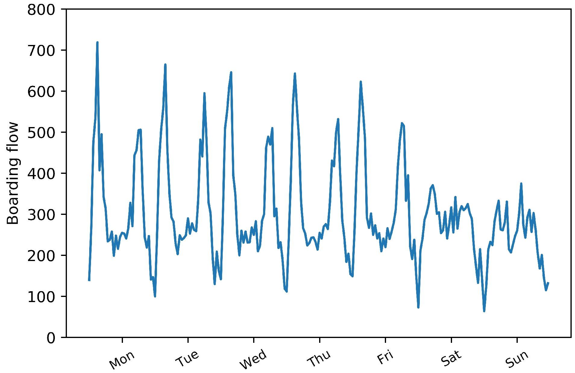
Figure 3 shows one week’s boarding flow in a region, that is the flow of each 30 min from 6:00 to 22:00 every day of one week. The region is located in the Beijing Central Business District, which is one of the busiest areas of Beijing. From the figure, we can find that there are two boarding-flow peaks every day during the weekday, and the boarding-flow curve is smoother during the weekend. Thus, there are obvious daily periodicity patterns. Figure 4 shows boarding flow in the same region of different time intervals, which is from 6:00 on 3 August 2015 to 22:00 on 30 August 2015. There are 896 time intervals. We can find that its period is 224 time intervals, i.e., one week. These all indicate that bus traffic flow has specific scenario patterns.
Figure 5 presents total bus traffic flow of all regions at each time interval. Each subgraph in the figure represents the total traffic flow of one day, which is the sum of bus alighting flow and boarding flow in all regions at each time interval. The horizontal coordinate in each subgraph represents different time intervals from 6:00 to 22:00, and the vertical coordinate in each subgraph represents the total traffic flow of the current time interval. There are a total of 28 subgraphs, representing 28 days from 3 August 2015 to 30 August 2015. The seven subgraphs of each column in the figure are all from Monday to Sunday.
From the figure, we can find that the bus traffic flow has two significant features that we define as bus scenario patterns. First, its total traffic flow volume is especially large and it has two peaks every day, which are from 7:30 to 9:30 in the morning and from 17:00 to 19:00 in the evening. Second, there are obviously different modes between workdays and weekends; the total traffic flow on the weekend is relatively small compared with the workday, and the traffic flow change is relatively smooth on the weekend compared with the workday. Therefore, it is crucial to capture the bus scenario patterns for traffic flow prediction.
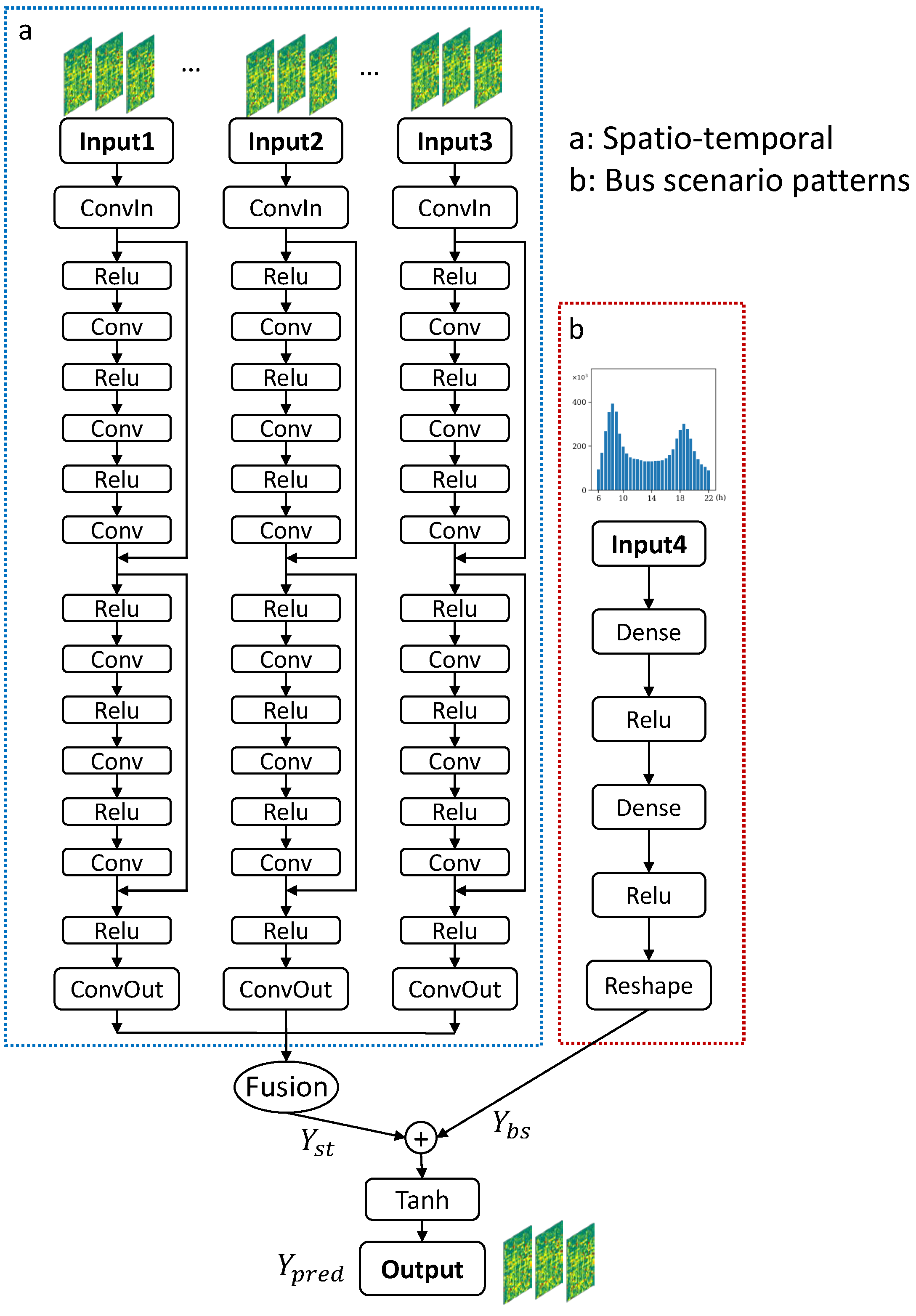
3.4. Building Our Model
Figure 6 presents the architecture of our proposed model, which is composed of four components. The left three components capture spatio-temporal correlation of bus traffic flow, which shared the same network structure. The single right component captures bus scenario patterns.
We first obtained the bus boarding flow and alighting flow of each time interval using Definition 1, which can stack together into a two-channel image-like matrix. Then, in order to capture the temporal correlation of bus traffic flow, we divided these matrices of all time intervals into three parts denoting adjacent time, near time, and far time, i.e., temporal closeness, period, and trend, respectively [10]. More specifically, to predict the of future time interval t, the closeness can be denoted as , which is a sequence that contains the past -length consecutive time interval observations. Then, we concatenated the sequence to a tensor , which is the input of Input1. Likewise, the period can be denoted as , which is a sequence that contains past -length observations with time interval of p, when p is set to one-day. The trend can be denoted as , which is a sequence that contains past -length observations with time interval of q, q is set to one-week. Then, the l-length sequence of closeness, period, and trend were concatenated into a tensor , respectively, which are inputs of the left three components, namely Input1, Input2, Input3.
The left three components share the same structure, that is each component contains a convolutional neural network layer named ConvIn, then connect to two improved residual blocks, and finally through a ReLU [19] activation function followed by another convolutional neural network layer named ConvOut; these convolutional networks can capture the spatial dependency of each region. The output of the left three components is weight-fused by the parametric-matrix-based method [10], which denotes the different influence of spatio-temporal correlations of each component to obtain the final spatio-temporal output .
The single right component of our model captures the bus scenario patterns. We first obtained the sum of bus boarding flow and alighting flow of each time interval, and then we normalized the flow sum and encode the normalized value into a one-dimension matrix, next we fed it into a two-layer fully connected neural network to get the output of bus scenario patterns . Then, we merge the spatio-temporal output and bus scenario patterns output , followed by a Tanh activation function. Finally, we obtained the prediction of bus traffic flow .
4. Experiments
In this section, we first describe our datasets, and then we present the evaluation metric and compared approaches. Next, we describe our experiment settings, including the data preprocessing and the detail of our training process, such as the hyperparameter settings. Finally, we show the performance of our proposed model compared with other baseline methods and analyze the results.
4.1. Datasets
Our datasets are Beijing transportation smart card data from 3 August 2015 to 30 August 2015, which contain about 177 million records of passengers’ bus transaction information. Each record contains the following key attributes: card id, bus route id, bus vehicle code, boarding and alighting time, latitude and longitude coordinates of boarding and alighting stations. We divided the metropolitan area of Beijing into grids, and each grid represents a region. The size of each region is 0.625 km × 0.625 km, and the time interval is set to half an hour. We filtered out night buses as there are quite few of them and the traffic flow is extremely small, then using Definition 1 we obtained bus boarding flow and alighting flow from 6:00 to 22:00 every day. The average and the max traffic flow of all regions were 87 and 3497, respectively. We choose the last four days as the test data and all date before that as the training data.
4.2. Evaluation Metric
In our experiment, we measure our method by root mean square error (RMSE) and mean average error (MAE), which are defined as follows:
where and are the ground truth and predicted value, respectively, and n is the number of all predicted values.
4.3. Compared Approaches
We compare our model with the following approaches:
Historical average (HA): HA predicts boarding flow and alighting flow for a given region using the average value of the previous relative time interval in the same region.
Autoregressive integrated moving average (ARIMA): ARIMA is a widely used method to predict future values in a time series. It combines autoregressive and moving average components for modeling time series.
DeepST [9]: DeepST is a deep neural network (DNN)-based prediction model for spatio-temporal data. It uses convolutional neural networks to predict spatio-temporal data.
ST-ResNet [10]: ST-ResNet is a deep residual network-based prediction model for spatio-temporal data. It employs deep residual network framework to model the spatio-temporal of crowd traffic.
4.4. Experiment Settings
The Beijing transportation smart card data are very large, containing about 177 million records of passengers’ bus transaction information. A single computer is too slow to process this, and sometimes even fails to produce results. We used the Apache Hadoop distributed computing platform, which consists of a cluster of eight Intel Xeon servers, to process the bus big data. We scaled the bus traffic flow value into the range [−1, 1] by the Min-Max normalization method. We re-scaled the predicted value back into the normal value in order to compare it with ground truth in the evaluation. The convolution kernel sizes were set to with 64 filters in the convolution layer of both ConvIn and improved residual block. The convolution kernel sizes were set to with two filters in ConvOut. We used the Tanh activation function in output weight layer, and the activation function in the other weight layers were ReLU [19]. The length of the three dependence sequences were set to , , and .
We trained our model in two stages. In the first stage, we split our training data into a 90% training set and 10% validation set, then we warmed up the training with 500 epochs, using early-stop methods to stop training when the validation metric stopped decreasing. Figure 7 presents the warm-up training, which shows the change of loss value and normalized RMSE value in each epoch, respectively. From the figure, we find that our proposed methods are very easy to train, and the training curves are close to the validation curves. After about 400 epochs, the training process was stopped, which showed that the validation metrics had stopped decreasing. In this way, we got the selected best model on the validation set. In the second stage, we continued training on all training data with another fixed number of epochs, e.g., 1000 epochs, using the selected best model. The learning rate was set to 0.0001. We used the Mean Squared Error as our loss function.
4.5. Performance Comparison
Table 1 shows the results of our proposed model, the improved spatio-temporal residual network (ISTR-Net) and its two variants compared with four baseline models. From the table, we can see that our model achieves the lowest RMSE and MAE, which proves that our proposed method can more effectively predict bus traffic flow than the baseline methods. More specifically, we can see that the predicted result of historical average (HA) is worst, which simply calculates the average value of historical flow in some previous relative time interval, for example, using all previous historical flow of 8:00 to 8:30 to predict 8:00 to 8:30, thus it cannot capture the temporal correlation of traffic flow effectively. Autoregressive integrated moving average (ARIMA) performs poorly when it just considers the temporal correlation of traffic flow, and overlooks the spatial correlation of traffic flow, such as the fact that traffic flow in one region may affect its adjacent region. For DeepST and ST-ResNet, we used the same hyperparameters with our proposed methods, we can see that DeepST and ST-ResNet, which use convolution neural networks to capture the spatio-temporal correlation of bus traffic flow, achieve better results than the traditional time-series method such as HA and ARIMA. However, these methods have not considered the bus scenario patterns. Compared with ST-ResNet, our proposed method uses improved residual blocks to model the spatio-temporal correlation of bus traffic flow effectively, while at the same time considering bus scenario patterns. Consequently, our proposed method outperforms those methods.
We also compare variants of our proposed method. There are two variants. In the first variant, we did not use the bus scenario patterns component which feeds nothing to the bus scenario patterns component, marked as none in the table. In the second variant, we encoded the metadata of weekday and weekend into one-hot values, and then fed the one-hot values instead of the flow sum value to the bus scenario patterns component to capture the scenario patterns, which is marked as metadata in the table. From the table, we can see that without the bus scenario patterns component, it performs poorly compared with our original method, which proves the effectiveness of the bus scenario patterns component. We also find that feeding one-hot encoded metadata of weekday and weekend cannot capture the bus scenario patterns, and it may lead to overfitting compared with the first variant, which also performs poorly. However, these two variants are all outperformed by the four baseline methods, which shows the effectiveness of our improved residual block. Therefore, we can see that it is important to capture both spatio-temporal correlation and its scenario patterns for bus traffic flow prediction, and our proposed method can synthetically capture spatio-temporal correlation and bus specific scenario patterns of bus traffic flow.
We further compared our proposed method with ST-ResNet during the rush hour period and off-peak period of the last four test days, that is from 27 August 2015 to 30 August 2015. As a result of the space limitation, we only show RMSE here, though we got the same conclusion of MAE. Figure 8 shows RMSE between ST-ResNet and our proposed method in rush hour (7:30–9:30), evening rush hour (17:00–19:00), and the off-peak period (12:00–14:00), respectively. From the figure, we can see that our proposed method has a lower RMSE compared with ST-ResNet, which shows that our proposed method has a better ability for bus traffic flow prediction in different periods. Moreover, we can see that prediction during rush hour is generally worse than the off-peak period. We believe that this is because the average value of traffic flow in rush hour is much larger than that of the off-peak period, e.g., 150 and 69 during rush hour and off-peak period, respectively. Because 27 August and 28 August are weekdays, and 29 August and 30 August are weekends, we can find that the prediction on weekdays are worse than weekends during rush hour, which we believe is because the average value of traffic flow on weekdays is larger than weekends, e.g., 123 and 82, respectively. However, the predictions on weekdays are better than weekends during the off-peak period; we think this is because the patterns are less regular on weekend.
5. Conclusions
In this paper, we build an improved spatio-temporal residual network to predict bus traffic flow. We find that bus traffic flow has a spatio-temporal correlation and specific scenario patterns. Our proposed method can synthetically capture the spatio-temporal correlation and bus specific scenario patterns of bus traffic flow. Specifically, we improve the residual network block to capture the spatio-temporal correlation of bus traffic flow effectively, and we use a fully connected neural network to capture the bus specific scenario patterns. The evaluation of our model on Beijing transportation smart card data shows that our proposed method achieves better results than the four baseline methods, which demonstrates that our proposed model performs better at predicting bus traffic flow.
However, there are still some improvements needed to our proposed method. The model can be improved by considering more heterogeneous data, such as point-of-interest data, social activities, and transportation networks. In addition, regions with similar functionality may have similar patterns; for example, tourist regions may have more traffic flow on weekends, and commercial regions may have more traffic flow in the evening. In the future, we will consider regions with similar functionality, and we will consider using local convolutional neural network in the same similar functional region to enhance the performance. Moreover, deep learning methods are often difficult to interpret, and it is interesting to understand and visualize the deep learning methods on traffic flow. We will consider visualizing the deep neural networks to understand how it learns the features of traffic flow.
Author Contributions
P.L. and Y.Z. conceptualized the work and defined the methodology; Y.Z. did the data curation; P.L. implemented the experiments and drafted the manuscript. Y.Z., D.K. and B.Y. operated the funding acquisition and contributed to the resources/supervision.
Funding
This work was supported in part by the National Natural Science Foundation of China under Grant U1811463, 4162009,61602486, 61632006, and 61772049, in part by the Beijing Municipal Science and Technology Project under Grant Z171100004417023, Z161100001116072, in part by the Beijing Municipal Education Project under Grant KM201610005033, and in part by the China Scholarship Council under Grant 201806540008.
Conflicts of Interest
The authors declare no conflict of interest.
References
- Ahmed, M.S.; Cook, A.R. Analysis of Freeway Traffic Time-Series Data by Using Box-Jenkins Techniques. Transp. Res. Rec. 1979, 722, 1–9. [Google Scholar]
- Kamarianakis, Y.; Prastacos, P. Forecasting traffic flow conditions in an urban network: Comparison of multivariate and univariate approaches. Transp. Res. Rec. J. Transp. Res. Board 2003, 1857, 74–84. [Google Scholar] [CrossRef]
- Kamarianakis, Y.; Prastacos, P. Space–time modeling of traffic flow. Comput. Geosci. 2005, 31, 119–133. [Google Scholar] [CrossRef] [Green Version]
- Kamarianakis, Y.; Shen, W.; Wynter, L. Real-time road traffic forecasting using regime-switching space-time models and adaptive LASSO. Appl. Stoch. Models Bus. Ind. 2012, 28, 297–315. [Google Scholar] [CrossRef]
- Chen, J.; Li, D.; Zhang, G.; Zhang, X. Localized Space-Time Autoregressive Parameters Estimation for Traffic Flow Prediction in Urban Road Networks. Appl. Sci. 2018, 8, 277. [Google Scholar] [CrossRef]
- Krizhevsky, A.; Sutskever, I.; Hinton, G.E. Imagenet classification with deep convolutional neural networks. In Proceedings of the Twenty-sixth Conference on Neural Information Processing Systems, Stateline, NV, USA, 3–8 December 2012; pp. 1097–1105. [Google Scholar]
- Luong, M.T.; Pham, H.; Manning, C.D. Effective approaches to attention-based neural machine translation. arXiv, 2015; arXiv:1508.04025. [Google Scholar]
- Wang, H.; Wang, N.; Yeung, D.Y. Collaborative deep learning for recommender systems. In Proceedings of the 21th ACM SIGKDD International Conference on Knowledge Discovery and Data Mining, Sydney, Australia, 10–13 August 2015; ACM: New York, NY, USA, 2015; pp. 1235–1244. [Google Scholar]
- Zhang, J.; Zheng, Y.; Qi, D.; Li, R.; Yi, X. DNN-based prediction model for spatio-temporal data. In Proceedings of the 24th ACM SIGSPATIAL International Conference on Advances in Geographic Information Systems, Burlingame, CA, USA, 31 October–3 November 2016; ACM: New York, NY, USA, 2016; p. 92. [Google Scholar]
- Zhang, J.; Zheng, Y.; Qi, D. Deep Spatio-Temporal Residual Networks for Citywide Crowd Flows Prediction. In Proceedings of the Thirty-First AAAI Conference on Artificial Intelligence (AAAI-17), San Francisco, CA, USA, 4–9 February 2017; pp. 1655–1661. [Google Scholar]
- He, K.; Zhang, X.; Ren, S.; Sun, J. Deep residual learning for image recognition. In Proceedings of the IEEE Conference on Computer Vision and Pattern Recognition, Las Vegas, NV, USA, 27–30 June 2016; pp. 770–778. [Google Scholar]
- He, K.; Zhang, X.; Ren, S.; Sun, J. Identity mappings in deep residual networks. In European Conference on Computer Vision; Springer: Cham, Switzerland, 2016; pp. 630–645. [Google Scholar]
- LeCun, Y.; Bengio, Y.; Hinton, G. Deep learning. Nature 2015, 521, 436–444. [Google Scholar] [CrossRef] [PubMed]
- Huang, W.; Song, G.; Hong, H.; Xie, K. Deep Architecture for Traffic Flow Prediction: Deep Belief Networks With Multitask Learning. IEEE Trans. Intell. Transp. Syst. 2014, 15, 2191–2201. [Google Scholar] [CrossRef]
- Lv, Y.; Duan, Y.; Kang, W.; Li, Z.; Wang, F.Y. Traffic flow prediction with big data: A deep learning approach. IEEE Trans. Intell. Transp. Syst. 2015, 16, 865–873. [Google Scholar] [CrossRef]
- Tan, H.; Xuan, X.; Wu, Y.; Zhong, Z.; Ran, B. A comparison of traffic flow prediction methods based on DBN. In CICTP 2016; American Society of Civil Engineers: Reston, VA, USA, 2016; pp. 273–283. [Google Scholar]
- Liu, L.; Chen, R.C. A novel passenger flow prediction model using deep learning methods. Transp. Res. Part C Emerg. Technol. 2017, 84, 74–91. [Google Scholar] [CrossRef]
- Ma, X.; Dai, Z.; He, Z.; Ma, J.; Wang, Y.; Wang, Y. Learning traffic as images: A deep convolutional neural network for large-scale transportation network speed prediction. Sensors 2017, 17, 818. [Google Scholar] [CrossRef] [PubMed]
- Nair, V.; Hinton, G.E. Rectified linear units improve restricted boltzmann machines. In Proceedings of the 27th International Conference on Machine Learning (ICML-10), Haifa, Israel, 21–24 June 2010; pp. 807–814. [Google Scholar]
- Chollet, F. Keras: The Python Deep Learning Library; Astrophysics Source Code Library: New York, NY, USA, 2018. [Google Scholar]
- Abadi, M.; Barham, P.; Chen, J.; Chen, Z.; Davis, A.; Dean, J.; Devin, M.; Ghemawat, S.; Irving, G.; Isard, M.; et al. Tensorflow: A system for large-scale machine learning. In Proceedings of the 12th USENIX Symposium on Operating Systems Design and Implementation (OSDI ’16), Savannah, GA, USA, 2–4 November 2016; Voume 16, pp. 265–283. [Google Scholar]
Figure 1.
Bus traffic flow matrix.

Figure 2.
Improved residual block.

Figure 3.
One week’s boarding flow in a region.

Figure 4.
Boarding flow of different time intervals in a region. The time interval is 30 min, starting from 6:00 on 3 August 2015.
Figure 4.
Boarding flow of different time intervals in a region. The time interval is 30 min, starting from 6:00 on 3 August 2015.

Figure 5.
Bus total traffic flow. Each subgraph represents the total traffic flow of all regions at each time interval in one day.
Figure 5.
Bus total traffic flow. Each subgraph represents the total traffic flow of all regions at each time interval in one day.

Figure 6.
The architecture of improved deep residual networks.

Figure 7.
Warm-up training on Beijing transportation smart card data. Left: The two curves denote training loss and validation loss, respectively. Right: The two curves denote training normalization root mean square error (RMSE) and validation normalization RMSE, respectively.
Figure 7.
Warm-up training on Beijing transportation smart card data. Left: The two curves denote training loss and validation loss, respectively. Right: The two curves denote training normalization root mean square error (RMSE) and validation normalization RMSE, respectively.

Figure 8.
RMSE of different periods between ST-ResNet and our proposed method.


Table 1.
Comparison with different baselines.
| Model | RMSE | MAE |
|---|---|---|
| HA | 44.66 | 21.52 |
| ARIMA | 30.31 | 20.96 |
| DeepST | 28.91 | 17.13 |
| ST-ResNet | 26.42 | 15.12 |
| ISTR-Net | 25.63 | 14.89 |
| ISTR-Net [none] | 25.76 | 14.93 |
| ISTR-Net [metadata] | 26.03 | 15.11 |
© 2019 by the authors. Licensee MDPI, Basel, Switzerland. This article is an open access article distributed under the terms and conditions of the Creative Commons Attribution (CC BY) license (http://creativecommons.org/licenses/by/4.0/).
Share and Cite
MDPI and ACS Style
Liu, P.; Zhang, Y.; Kong, D.; Yin, B. Improved Spatio-Temporal Residual Networks for Bus Traffic Flow Prediction. Appl. Sci. 2019, 9, 615. https://doi.org/10.3390/app9040615
AMA Style
Liu P, Zhang Y, Kong D, Yin B. Improved Spatio-Temporal Residual Networks for Bus Traffic Flow Prediction. Applied Sciences. 2019; 9(4):615. https://doi.org/10.3390/app9040615
Chicago/Turabian StyleLiu, Panbiao, Yong Zhang, Dehui Kong, and Baocai Yin. 2019. "Improved Spatio-Temporal Residual Networks for Bus Traffic Flow Prediction" Applied Sciences 9, no. 4: 615. https://doi.org/10.3390/app9040615
Note that from the first issue of 2016, this journal uses article numbers instead of page numbers. See further details here.