Fast 3D Semantic Mapping in Road Scenes ^†

Abstract

Fast 3D reconstruction with semantic information in road scenes is of great requirements for autonomous navigation. It involves issues of geometry and appearance in the field of computer vision. In this work, we propose a fast 3D semantic mapping system based on the monocular vision by fusion of localization, mapping, and scene parsing. From visual sequences, it can estimate the camera pose, calculate the depth, predict the semantic segmentation, and finally realize the 3D semantic mapping. Our system consists of three modules: a parallel visual Simultaneous Localization And Mapping (SLAM) and semantic segmentation module, an incrementally semantic transfer from 2D image to 3D point cloud, and a global optimization based on Conditional Random Field (CRF). It is a heuristic approach that improves the accuracy of the 3D semantic labeling in light of the spatial consistency on each step of 3D reconstruction. In our framework, there is no need to make semantic inference on each frame of sequence, since the 3D point cloud data with semantic information is corresponding to sparse reference frames. It saves on the computational cost and allows our mapping system to perform online. We evaluate the system on road scenes, e.g., KITTI, and observe a significant speed-up in the inference stage by labeling on the 3D point cloud.

1. Introduction

Scene understanding plays a key background role in most vision-based mobile robots. For example, autonomous navigation in indoor/outdoor scenes asks for a rapid and comprehensive understanding of surroundings for obstacle avoidance and path planning [1,2,3]. Vehicle movement in limited temporal and spatial contexts always requires knowledge of what there are around ego-vehicle and where it is located. Robotic maps, such as Occupancy grid map and OctoMap, traditionally provide geometric presentation of the environment. However, they lack the correlation in data between map points and semantic knowledge; thus, they could not be directly utilized for scenes understanding.

Scene parsing/semantic segmentation is an important and promising step to address this issue. It has been an active topic for a long time, and it benefits from the state-of-the-art Deep Convolutional Neural Networks (DCNNs), which contributes to better performance of 2D pixel labeling than traditional methods. Then, combined with the SLAM technology, an automobile could locate itself and meanwhile recognize surrounding objects on a pixel-wise level. For instance, it could make autonomous vehicle accomplish certain high-level tasks, such as “parking on the right free space” and “stopping at the crosswalk”. This form of 3D semantic representation provides mobile robots with functions of understanding, interaction, and navigation in various scenes.

Most semantic segmentation methods focus on increasing the accuracy of the semantic segmentation, and have seen major improvements [4,5]. However, they usually asks for high-power computing resources, which is not suitable for embedded platforms. Several recent research try to make a balance between the computing cost and the accuracy of object detection, classification, and 2D pixel labeling [6,7]. They achieve better performance on the embedded and mobile platforms.

Visual SLAM is a promising technology, especially based on monocular vision, which is flexible, inexpensive, and widely equipped on most recent vehicles. Although scaled sensors like stereo cameras and RGB-Depth (RGB-D) cameras could provide reliable measurement in their specific ranges, they lack the capability of seamless switch between various-scaled scenes. In addition, they normally need large storage resources. Most man-made environments, e.g., road scenes, usually exhibit distinctive spatial relations among varied classes of objects. Employing theses relations could enhance semantic segmentation performance in the 3D semantic mapping [8]. In this paper, we exploit a monocular SLAM method that provides cues of 3D spatial information and utilize state-of-the-art DCNN to build a 3D scene understanding system towards road scenes. Moreover, a Bayesian 2D-3D transfer and a map regularization process are utilized to generate a consistent reconstruction in the spatial and semantic context.

In our monocular mapping system, the map is incrementally reconstructed with a sequence of automatically selected keyframes and corresponding semantic information. There is no need to label each frame in a sequence, which could save a considerable amount of computation cost. We refer readers to Figure 1. Different from the frame skipping strategy proposed by Hermans et al. [9] and McCormac et al. [10], our method could work well under fast motions. Since the 3D map should have global consistent depth information, it should be regularized in term of spatial structures. The regularization is aimed at removing distinctive outliers and it makes components more consistent in the point cloud map, i.e., local points with same semantic label should be approached in 3D space. Two datasets, Cityscapes [11] and KITTI [12], are used to evaluate our approach. This work is an extension of our previous work [13]. We not only modify the 2D semantic segmentation module, but also revise the offline regularization module with new potential constraint. More experiments and theoretical details are involved in this work. The main contributions involve the improvement of 2D semantic segmentation model, the associative hierarchical Conditional Random Field (CRF) with High Order Potential towards the point cloud, the extended experiments and the quantitative evaluation of the performance including accuracy and runtime.

This paper is presented as follows. In the Section 2, a review of the related work is given. The problem formulation is presented in Section 3. The 3D semantic mapping is described in Section 4, including the semantic segmentation, the monocular visual SLAM, the Bayesian incremental fusion, and the global regularization. Section 5 includes the results of 2D semantic inference and 3D semantic mapping. Finally, Section 6 concludes the paper and discusses possible extensions of our work.

2. Related Work

Our work is motivated by [10] which contributes an indoor 3D semantic SLAM from the RGB-D input. It aims towards a dense 3D map based on ElasticFusion SLAM [14] with semantic labeling. Pixel-wise semantic information is acquired from a Deconvolutional semantic segmentation network [15] using the scaled RGB information and the depth as the input. Depth information is also used to update surfel’s depth and normal information to construct 3D dense map during loop closure. In addition, a previous work, SLAM++ [16], creates a map with semantically defined objects, but it is limited to predefined database and hand-crafted template models. In this paper, we make use of an incremental Bayesian fusion strategy with state-of-the-art visual SLAM and semantic segmentation.

Visual SLAM usually contains sparse, semi-dense, and dense types depending on the methods of image alignment. Feature-based methods only exploit limited feature points—typically image corners and blobs or line segments, such as classic MonoSLAM [17] and ORB-SLAM [18,19]. They are not suitable for 3D semantic mapping due to rather sparse feature points. In order to better exploit image information and avoid the cost on calculation of features, direct dense SLAM system, such as the surfel-based dense slam, ElasticFusion [14], and Dense Visual SLAM [20], have been proposed recently. Whereas, direct image alignment from these dense methods is well-established for monocular, RGB-D and stereo sensors. Semi-dense methods like Large-Scale Direct-SLAM (LSD-SLAM) [21] and Semi-direct Visual Odometry (SVO) [22] provide possibility to build a synchronized 3D semantic mapping system.

Deep CNNs have proven to be effective in the field of image semantic segmentation. Long et al. [23] firstly introduces an inverse convolution layer to realize an end-to-end training and inference. Then, the encoder-decoder architectures with specified upsampling layers, such as max unpooling and deconvolutional layer, are proposed to avoid the problem of separate step training in the Fully Convolutional Network (FCN) and improve the accuracy [15,24]. Zhao et al. [4] exploit the capability of global context information through embedding various scenery context feature in a pyramid structure. The fusion of varied scaled feature has been a popular strategy in the recent deep CNNs. The cutting-edge method, namely, DeepLab series [5,7], combines atrous convolutions and atrous spatial pyramid pooling (ASPP) to achieve a state-of-the-art performance on semantic segmentation. The early DeepLab models have a reasonable accuracy but require much computation overhead. Recently proposed efficient convolution neural network, such as MobileNets [25,26] boosts real-time performance of semantic segmentation without losing the accuracy too much. The state-of-the-art DeepLab-v3+ [7] contains a simple effective decoder module to refine the segmentation results especially along object boundaries. Furthermore, combining the encoder part of MobileNet-v2 in its structure, DeepLab-v3+ could achieve a better trade-off between precision and runtime.

In the topic of scene understanding and mapping, recent researchs employ 3D priors of objects increasingly. Salas-Moreno et al. [16] project 3D mesh of objects to the RGB-D frame in a graphical SLAM framework. Valentin et al. [27] propose a triangulated meshed representation of the scene from multiple depth measurements and exploit the CRF to capture the consistency of 3D object mesh. Kundu et al. [28] exploit the CRF for joint voxels to infer the semantic information and occupancy. Sengupta and Sturgess [29] use stereo camera, estimated pose, and CRF to infer the semantic octree presentation of the 3D scene. Vineet et al. [30] propose an incremental dense stereo reconstruction and semantic fusion technique to handle dynamic objects in the large-scale outdoor scenes. Kochanov et al. [31] employ scene flow measurements to incorporate temporal updates into the mapping of dynamic environment. Landrieu et al. [32] introduce a regularization framework to obtain spatially smooth semantic labeling of 3D point clouds from a point-wise classification, considering the uncertainty associated with each label. Gaussian Process (GP) is another popular method for map inference. Jadidi et al. [33] exploit GP to learn the structural and semantic correlation between map points. This technique also incorporates OcotoMap to handle sparse measurements and missing labels. In order to improve the training and query time complexities of the GP-based semantic mapping, Gan et al. [34] further introduce a Relevance Vector Machine (RVM) inference technique for efficient map query at any resolution.

Our semi-dense approach is also inspired by dense 3D semantic mapping methods [8,9,35,36] in both indoor and outdoor scenes. The major contributions from these work involve the 2D-3D transfer and the map regularization. Especially, Hermans et al. [9] propose an efficient 3D CRF to regularize 3D semantic mapping consistently considering influence between neighbors of 3D points (voxels). In this work, we adopt a similar strategy to improve the performance of the 3D semantic reconstruction in the road scenes. The key concepts are

• a 3D semantic mapping system based on monocular vision,
• integration of monocular SLAM [21] and scene parsing [7] into 3D semantic representation,
• exploiting the correlation between semantic information and geometrical information to enforce spatial consistency,
• active sequence downsampling and sparse semantic segmentation so that to achieve a real-time performance and reduce the storage.

Following the comparison in [30], we list the characteristics of our approach and some related works in

Table 1. Comparison with some related work: M = monocular camera, S/D = stereo/depth camera, L = lidar, O = outdoor, I = incremental, SDT = sparse data structures, RT = real time.

Method	M	S/D	L	O	I	SDT	RT
Hu et al. [37]			√	√	√	√	√
Sengupta et al. [35]		√		√
Hermans et al. [9]		√			√		√
Kundu et al. [28]	√			√		√
Vineet et al. [30]		√		√	√	√	√
Wolf et al. [8]		√					√
McCormac et al. [10]		√			√	√	√
Ours	√			√	√	√	√

.

3. Problem Formulation

3.1. Notation

The target is to estimate the 3D semantic map $\mathcal{M}$ comprising of a pose-graph of keyframes with semantic map from a monocular camera. The 3D map $\mathcal{M}$ is reconstructed by the estimation of depth and poses, where each 3D point $\mathbf{P}$ can be labeled as one of the solid semantic objects in the label space $\mathcal{L}=\{l_1,l_2,\dots ,l_k\}$ like Road, Building, Tree, etc. We use $\mathbf{X}=\{X_1,X_2,\dots ,X_M\}$ to denote the set of random variables corresponding to the 3D points ${\mathbf{P}}_i:i\in \{1,\dots ,M\}$, where each variable $X_i\in \mathbf{X}$ take a value $l_i$ from the predefined label space $\mathcal{L}$.

Let $I_i:{\mathsf{\Omega }}_i\to {\mathbb{R}}^3$ symbolize an $\mathrm{H}\times \mathrm{W}$ RGB image of an input sequence at the frame indexed by i. Keyframes are extracted from the sequence in light of camera’s pose ${\mathbf{T}}_i^j$ at the jth frame with respect to the previous ith keyframe. We define the ith keyframe to be a tuple ${\mathcal{K}}_i=(I_i,D_i,V_i,S_i)$, where $D_i:{\mathsf{\Omega }}_{D_i}\to \mathbb{R}$ is the full-resolution inverse depth map associated with image $I_i$, and $V_i:{\mathsf{\Omega }}_{V_i}\to \mathbb{R}$ is the variance associated with the inverse depth map. The inverse depth model is a better description for visual depth estimation, which assumes normally distributed [38]. The inverse depth map and the variance map are defined in the subset of pixels as ${\mathsf{\Omega }}_{D_i},{\mathsf{\Omega }}_{V_i}\subset {\mathsf{\Omega }}_i$, which means semi-dense, available for certain image regions of large intensity gradient. The symbol $S_i:{\mathsf{\Omega }}_{S_i}\to {\mathbb{R}}^{|\mathcal{L}|}$ represents the full-resolution semantic map with the probability of each object class.

The keyframes are consecutively stacked in a pose-graph $\mathcal{G}=(\mathcal{V},\mathcal{E})$, where $\mathcal{V}=\{{\mathcal{K}}_0,\dots ,{\mathcal{K}}_n\}$ is the set of keyframes and $\mathcal{E}=\{{\mathbf{S}}_i^j\in \mathrm{Sim}(3):{\mathcal{K}}_i,{\mathcal{K}}_j\in \mathcal{V}\}$ is the set of constraint factors. Each ${\mathbf{S}}_i^j=({\mathbf{T}}_i^j,s_i^j)$ consists of a camera’s pose ${\mathbf{T}}_i^j=\left(\genfrac{}{}{0pt}{}{Rt}{01}\right)$ from the keyframe ith to the keyframe jth, and scale factor $s_i^j>0$. In reference to world frame W, regarded as the pose of the first keyframe ${\mathcal{K}}_0$, the pose of the keyframe ith is denoted as ${\mathbf{T}}_W^i$. For a sequence of keyframes (n keyframes), we get the nth keyframe’s pose ${\mathbf{T}}_W^n={\prod }_1^n{\mathbf{T}}_{k-1}^k$.

3.2. Framework

Our target is to build a 3D semantic map with semi-dense and consistent label information online while the image sequences are captured by a forward-moving monocular camera. Given an image sequence, the inference of the 3D semantic map is regarded as:

$${\mathcal{M}}^{*}={\mathrm{argmax}}_{\mathcal{M}}P(\mathcal{M}|\mathcal{G}),$$

(1)

which can be estimated by the maximum a-posterior (MAP). Compared to the model used in [28], our measures are continually updated with new keyframes. Thus, we adopt an incremental fusion strategy to estimate the 3D semantic map by incorporating new estimation of pose, depth, and semantic information. Correspondingly, the approach is decoupled into three separately running processes as shown in Figure 2.

In the system, the monocular SLAM process maintains and tracks on a global map of the environment, which contains a number of keyframes connected by pose-pose constraints with associated probabilistic depth maps. It runs in real-time on a CPU. Represented as point clouds, the map gives a semi-dense and highly accurate 3D reconstruction of the environment. Meanwhile, the second process of the 2D semantic segmentation generates the pixel-level classification on the extracted keyframes. A fast deep CNN model is explored to predict the semantic information on a GPU. In addition, an incremental fusion process for the semantic label optimization is operated in a parallel way. It builds a local optimal correspondence between semantic labeling and 3D points in the point cloud. To obtain a globally optimal 3D semantic segmentation, we attempt to make use of information of neighboring 3D points, involving the distance, color similarity, and semantic label. It optimizes the point cloud and semantic labels to generate a globally consistent 3D semantic map.

4. 3D Semantic Mapping

4.1. 2D Scene Parsing

We explore the DeepLab-v3+ deep neural network proposed by Chen et al. [7]. Two important components in the DeepLab series are the atrous convolution and atrous spatial pyramid pooling (ASPP), which enlarge the field of view of filters and explicitly combine the feature maps at multiple scales. The improvement in the DeepLab-v3+ involves the encoder-decoder structure and the augmentation of ASPP module with image-level feature. The former is able to capture sharper object boundaries by regaining the spatial information, while the latter encodes multi-scale contextual information to capture long range information. These contributions make DeepLab successfully handle both large and small objects and achieve a better trade-off between precision and run-time.

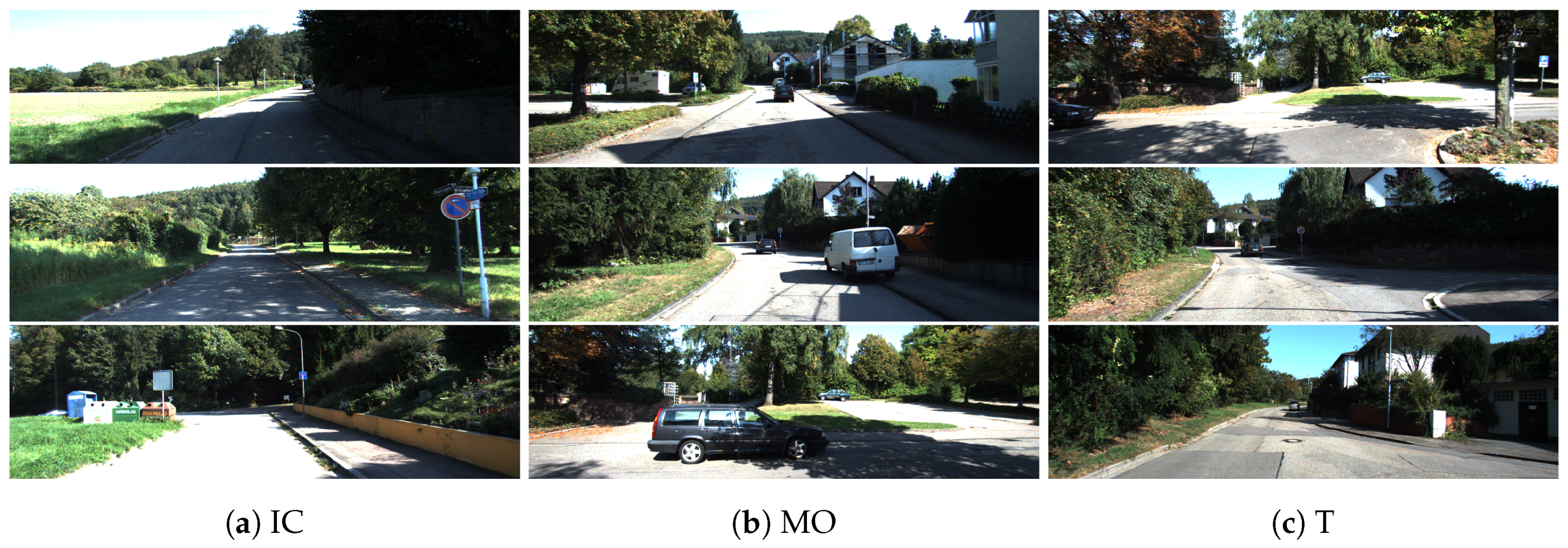
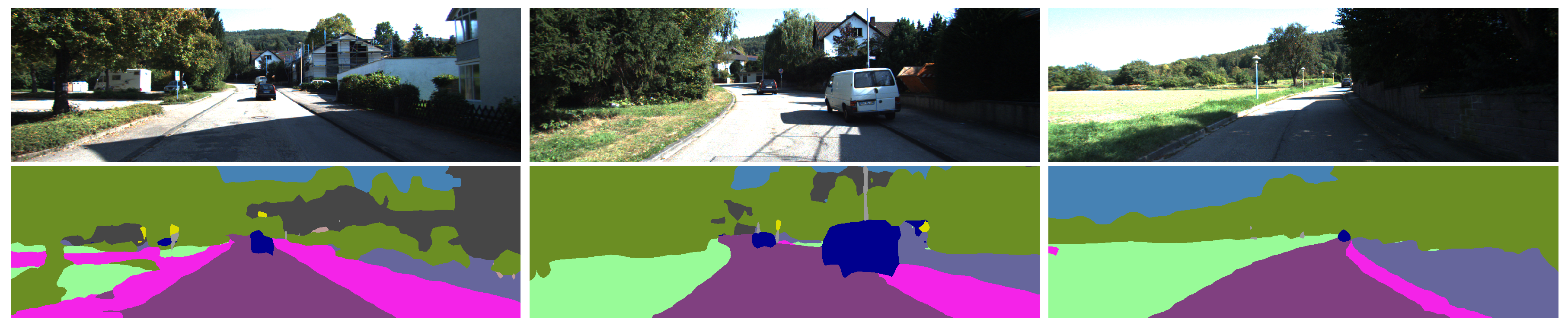
For the semantic segmentation of road scenes, we exploit the Cityscapes dataset and the KITTI dataset and adopt the predefined 19-class label space $\mathcal{L}=\{l_1,l_2,\dots ,l_{19}\}$, which contains Road, Sidewalk, Building, Wall, and so on. We use all semantic annotated images in the Cityscapes dataset for training and fine-tune the model with the KITTI dataset. Note that there is not any depth information involved in the training process. In the inference, we keep the original resolution of input image according to different datasets.

4.2. Semi-Dense SLAM

We explore LSD-SLAM to track camera’s trajectory and build consistent, large-scale maps of the environment. LSD-SLAM is a real-time, semi-dense 3D mapping method. It has several advantages: firstly, it is a scale-aware image alignment algorithm to directly estimate the similarity transform between two keyframes against different scale environments, such as office rooms (indoor) and urban roads (outdoor). The second one is that it is a probabilistic approach to incorporate noise on the estimated inverse depth maps into the tracking based on the propagation of uncertainty. Moreover, it could easily integrate with various kinds of sensors like monocular, stereo and panoramic cameras for various applications. Thus, it is able to make a reliable trajectory estimation and map reconstruction even in challenging surroundings.

LSD-SLAM has three major components: tracking, depth estimation and map optimization. Spatial regularization and outlier removal are incorporated in the depth estimation with small-baseline stereo comparisons. In addition, a direct, scale-drift aware image alignment is carried on these existing keyframes to detect scale-drift and loop closures. Due to the inherent correlation between the depth and the tracking accuracy, depth residual is used to estimate the similarity transform $\mathfrak{sim}(3)$ constraints between keyframes. Consequently, a 3D point cloud map is built based on a set of keyframes with the estimated inverse depth maps via minimizing the error of image alignment. The map is continuously optimized in the background using a g2o pose-graph optimization. The approach runs at 25 Hz on an Intel i7 CPU. More details like keyframe selection and depth estimation can be referred to the work [21].

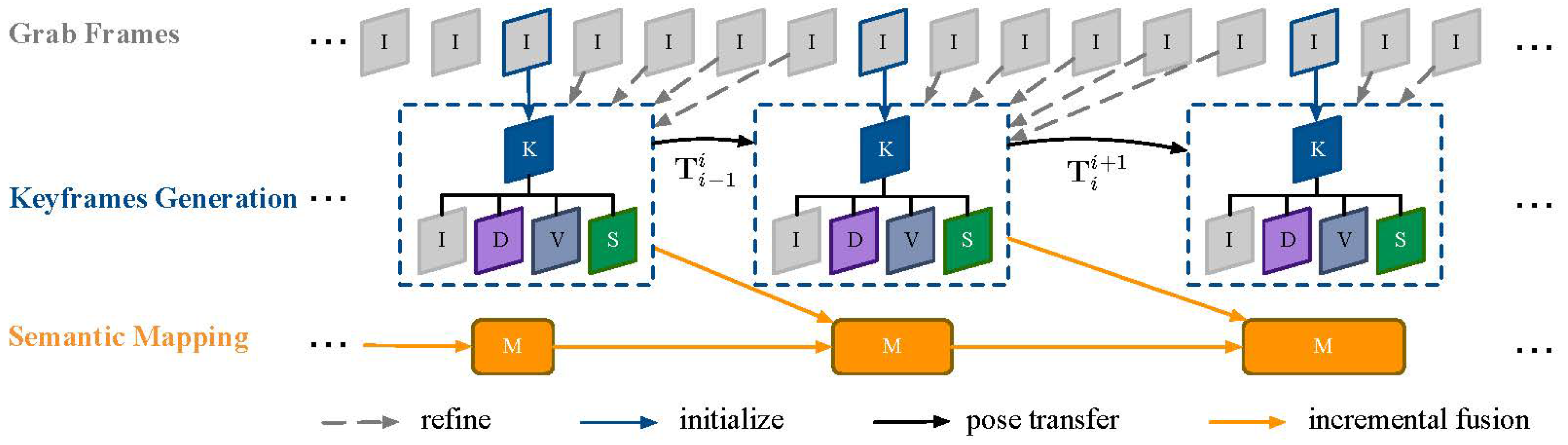
4.3. Incremental Fusion

There might be a large amount of inconsistent 2D semantic labels between consecutive frames, due to the noise of sensors, the complexity of environments in the real world and the failure of scene parsing model. Incremental fusion of semantic label from the stacked keyframes allows associating probabilistic label in a Bayesian way, when combining with the inverse depth map propagation between keyframes in the LSD-SLAM. We give the details about the incremental semantic fusion as follows.

The camera projection transformation function $\pi (·):{\mathbb{R}}^3\to {\mathbb{R}}^2$ is defined as

$$\mathbf{p}=\pi (\mathbf{P})={[\alpha \frac{x}{z}+c_x,\beta \frac{y}{z}+c_y]}^T,$$

(2)

which maps a point $\mathbf{P}={[x,y,z]}^T$ in 3D space into a 2D point $\mathbf{p}={[x^{\prime },y^{\prime }]}^T$ on the digital image plane $I_i$ in the camera coordinate system. Since this projection function is nonlinear, for the computation efficiency, the transformation should be augmented into the homogeneous coordinate system, which is defined as

$${\mathbf{p}}_h=\left[\begin{array}{c}{x}_h^{\prime }\\ y_h^{\prime }\\ z_h^{\prime }\end{array}\right]=\left[\begin{array}{cccc}\alpha & 0& c_x& 0\\ 0& \beta & c_y& 0\\ 0& 0& 1& 0\end{array}\right]\left[\begin{array}{c}x\\ y\\ z\\ 1\end{array}\right]=\mathbf{K}[\mathbf{I}0]{\mathbf{P}}_h,$$

(3)

where $\mathbf{K}$ is referred to as the camera matrix. Given a 3D point ${\mathbf{P}}_W$ in the world reference system, the mapping to image plane $I_i$ in the homogeneous reference system is calculated as

$${\mathbf{p}}_h=\mathbf{K}{\mathbf{T}}_W^i{\mathbf{P}}_{Wh},$$

(4)

where ${\mathbf{T}}_W^i$ is the pose of the camera in the world reference system. Then, we get Euclidean coordinates $\mathbf{p}={[x_h^{\prime }/z_h^{\prime },y_h^{\prime }/z_h^{\prime }]}^T$ from the homogeneous coordinates. From this point on, any point $\mathbf{p}$ and $\mathbf{P}$ is assumed to be in homogeneous coordinates and thus we drop the h index, unless stated otherwise.

Correspondingly, given the inverse depth estimation $\widehat{d}$ for a pixel $\mathbf{p}={[x^{\prime },y^{\prime }]}^T$ in the image $I_i$ of the keyframe ${\mathcal{K}}_i$, we also have an inverse projection function from 2D pixel point into the 3D point in the current camera coordinate system as:

$$\mathbf{P}={\pi }^{-1}(\mathbf{p},\widehat{d})={[\frac{x^{\prime }/\widehat{d}-c_x/\widehat{d}}{\alpha },\frac{y^{\prime }/\widehat{d}-c_y/\widehat{d}}{\beta },\frac{1}{\widehat{d}}]}^T,$$

(5)

where $\widehat{d}=D_i(\mathbf{p})\sim \mathcal{N}(\mu ,V_i(\mathbf{p}))$ corresponds to the inverse depth of the point $\mathbf{p}$, which is normally distributed. The inverse depth estimation of each existing keyframe is continuously refined using its following frames until new keyframe is selected. In reference to Equations (4) and (5), we can derive the normally distributed 3D points in the world reference system as follows:

$${\widehat{\mathbf{P}}}_W={T_W^i}^{-1}{\pi }^{-1}(\mathbf{p},D_i(\mathbf{p}),V_i(\mathbf{p})),$$

(6)

where the homogeneous transformation matrix has the property: ${T_W^i}^{-1}=T_i^W$.

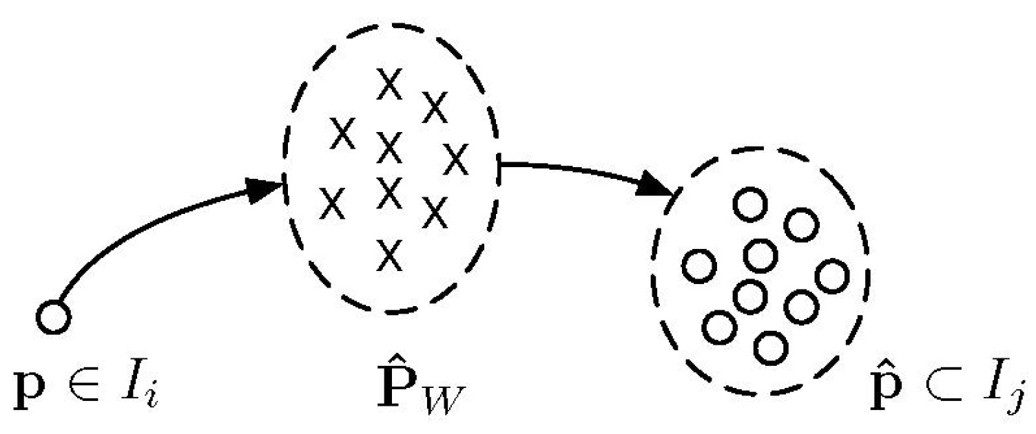
Once a new frame is chosen to become a keyframe ${\mathcal{K}}_j$, its inverse depth map $D_j$ is initialized by projecting points from previous keyframe into it. The information of existing, close-by keyframes is propagated to new keyframe for its initialization and semantic probabilistic refinement. The corresponding point $\widehat{\mathbf{p}}$ in the image $I_j$ of new keyframe is located by

$$\widehat{\mathbf{p}}=\mathbf{K}{\mathbf{T}}_W^i{\mathbf{T}}_i^j{\widehat{\mathbf{P}}}_W\in I_j.$$

(7)

Here, since the estimation of the inverse depth map is normally distributed, we have a one-to-many transform between keyframes, which involves a couple of estimated 2D/3D points, regarded as $\mathbf{p}\in I_i\to {\widehat{\mathbf{P}}}_W\to \widehat{\mathbf{p}}\subset I_j$, as shown in Figure 3.

The class label corresponding to a couple of 3D points ${\widehat{\mathbf{P}}}_W$ in the world reference is denoted as $X:{\widehat{\mathbf{P}}}_W\to l\in \mathcal{L}$. Note that the label $Sky$ is removed from $\mathcal{L}$ for the 3D semantic mapping. Our target is to obtain the independent probability distribution of each 3D point over the class labels $P(X|{\mathcal{K}}_0^i)$ given a sequence of existing keyframes ${\mathcal{K}}_0^i=\{{\mathcal{K}}_0,{\mathcal{K}}_1,\dots ,{\mathcal{K}}_i\}$ in the pose-graph $\mathcal{G}$.

We explore a recursive Bayesian fusion to refine the corresponding probability distribution of 3D points with new keyframe’s update:

$$P(X|{\mathcal{K}}_0^i)=\frac{1}{Z_i}P({\mathcal{K}}_i|{\mathcal{K}}_0^{i-1},X)P(X|{\mathcal{K}}_0^{i-1}),$$

(8)

with $Z_i=P({\mathcal{K}}_i|{\mathcal{K}}_0^{i-1})$. Applying the first-order Markov assumption to $p({\mathcal{K}}_i|{\mathcal{K}}_0^{i-1},X)$, then we have:

$$P(X|{\mathcal{K}}_0^i)=\frac{1}{Z_i}P({\mathcal{K}}_i|X)P(X|{\mathcal{K}}_0^{i-1})=\frac{1}{Z_i}\frac{p({\mathcal{K}}_i)P(X|{\mathcal{K}}_i)}{P(X)}P(X|{\mathcal{K}}_0^{i-1}).$$

(9)

We assume that $P(X)$ does not change over time and there is no need to calculate the normalization factor $P({\mathcal{K}}_i)/Z_i$ explicitly.

According to the formulations above, the semantic probability distribution of all given keyframes can be recursively updated as follows:

$$P(X|{\mathcal{K}}_0^i)\propto P(X|{\mathcal{K}}_i)P(X|{\mathcal{K}}_0^{i-1}),$$

(10)

where a couple of 2D pixels matching between ${\mathcal{K}}_0^i$ can be calculated with the Equations (4) and (5). The semantic map in ${\mathcal{K}}_0^i$ contributes to the accumulated probabilistic estimation of object class. For example, given a pixel $\mathbf{p}$ in the image $I_i$ of the keyframe ${\mathcal{K}}_i$, its corresponding scores (probabilities) of object classes are $S_i(\mathbf{p})=\{P(Road|\mathbf{p})=p_1,P(Sidewalk|\mathbf{p})=p_2,P(Building|\mathbf{p})=p_3,\dots ,P(Bicycle|\mathbf{p})=p_{19}\}$ with $\sum p_i=1$. Then, at each fusion step, the predicted labels of 3D point ${\widehat{\mathbf{P}}}_W$ is the label with maximum probabilities as

$$\underset{k=1}{\overset{N}{max}}{S}_j({\widehat{\mathbf{p}}}_k)S_i(\mathbf{p}),$$

(11)

where there are N possible projected 3D points and pixels $\widehat{\mathbf{p}}$ in the image $I_j$ of the keyframe ${\mathcal{K}}_j$.

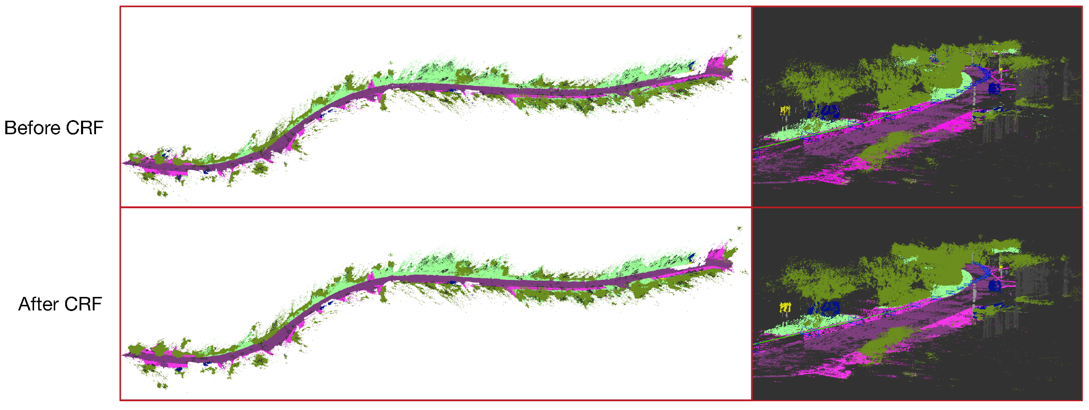
The incremental fusion can refine the semantic label of the points in the 3D space based on the pose-graph of keyframes. It could handle the inconsistent 2D semantic labels, even though its performance relies on the depth estimation. In addition, map geometry is another useful feature which could improve the performance of the 3D semantic mapping further. The following section describes how we use the dense CRF to regularize the 3D semantic map by exploring the map geometry, which could propagate semantic information between spatial neighbors.

4.4. Map Regularization

The dense CRF is widely used in the 2D semantic segmentation to enhance the performance of semantic segmentation. Some previous works [8,9,35] seek its application on the 3D map to model contextual relations between various class labels in a fully connected graph. It is a heuristic approach that assumes the influence between neighbors should be proportional to their distance, visual, and geometrical similarity [9].

The CRF model is defined as a graph composed of unary potentials as nodes and pairwise potentials as edges, but the size of the model makes traditional inference algorithms impractical. Thanks to Krahenbuhl and Koltun’s work [39], a highly efficient approximate inference algorithm is proposed to handle this issue by defining the pairwise edge potentials as a linear combination of Gaussian kernels. We apply the efficient inference of the dense CRF to maximize label agreement between similar 3D points as follows.

Assume the 3D semantic map $\mathcal{M}$ containing M 3D points is defined as a random field. A CRF $(\mathcal{M},\mathbf{X})$ is characterized by a Gibbs distribution as follows:

$$P(\mathbf{X}|\mathcal{M})=\frac{1}{Z(\mathcal{M})}exp(-E(\mathbf{X}|\mathcal{M})),$$

(12)

where $E(\mathbf{X}|\mathcal{M})$ is the Gibbs energy and $Z(\mathcal{M})$ is the partition function. The maximum a posteriori (MAP) labeling of the random field is

$${\mathbf{X}}^{*}={\mathrm{argmax}}_{l\in \mathcal{L}}P(\mathbf{X}|\mathcal{M})={\mathrm{argmin}}_{l\in \mathcal{L}}E(\mathbf{X}|\mathcal{M}),$$

(13)

which is converted into minimizing the Gibbs energy by the mean-field approximation and message passing scheme.

We employ the associative hierarchical CRF [35,40] which integrates the unary potential ${\psi }_i$, the pairwise potential ${\psi }_{i,j}$, and the higher order potential ${\psi }_c$ into the Gibbs energy at different levels of the hierarchy (voxels and supervoxels) given by:

$$E(\mathbf{X}|\mathbf{C};\theta )=\sum _i{\psi }_i(X_i|\mathbf{C})+\sum _{i<j}{\psi }_{i,j}(X_i,X_j|\mathbf{C};\theta )+\sum _c{\psi }_c(X_c|\mathbf{c})$$

(14)

by the indexes $i,j\in \{1,\dots ,M\}$ correspond to different 3D points ${\mathbf{P}}_i,{\mathbf{P}}_j$ in the 3D map $\mathcal{M}$.

Unary Potential: The unary potential ${\psi }_i(·)$ is defined as the negative logarithm of the probabilistic label for a given 3D point:

$${\psi }_i(X_i|\mathbf{C})=-log(P(X_i\to l|{\mathcal{K}}_0^t)).$$

(15)

This term means the cost of 3D point $P_i$ taking an object label $l\in \mathcal{L}$ based on the incremental semantic probabilistic fusion above. The output of the unary potential for each point is produced independently, and thus, the MAP labeling produced by the unary potential alone is generally inconsistent.

Pairwise Potentials: The pairwise potential ${\psi }_{i,j}(·)$ is modeled to be a log-linear combination of m Gaussian edge potential kernels:

$${\psi }_{i,j}(X_i,X_j|\mathbf{C};\theta )=\mu (X_i,X_j)\sum _m{\omega }^{(m)}{k}^{(m)}({\mathbf{f}}_i,{\mathbf{f}}_j;\theta ),$$

(16)

where $\mu (·)$ is a label compatibility function corresponding to the Gaussian kernel functions $k^{(m)}({\mathbf{f}}_i,{\mathbf{f}}_j)$. $\mathbf{f}$ denotes the feature vector for the 3D point $\mathbf{P}$ including the position, the RGB appearance and the surface normal vector of the reconstructed surface. Furthermore, $\mu (·)$ is defined as a Potts model given by:

$$\mu (l,l^{\prime })=[l\ne l^{\prime }]=\left\{\begin{array}{cc}1\hfill & l\ne l^{\prime }\hfill \\ 0\hfill & l=l^{\prime }\hfill \end{array}\right..$$

(17)

This term is defined to encourage the consistency over pairs of neighboring points for the local smoothness of the 3D semantic map. We employ two Gaussian kernels for the pairwise potentials following the previous work [9]. The first one is an appearance kernel as follows:

$$k^{(1)}({\mathbf{f}}_i,{\mathbf{f}}_j;\theta )=\exp \left(-\frac{|{\mathbf{P}}_i-{\mathbf{P}}_j{|}^2}{2{\theta }_{\mathbf{P},c}^2}-\frac{|{\mathbf{c}}_i-{\mathbf{c}}_j{|}^2}{2{\theta }_c^2}\right),$$

(18)

where $\mathbf{c}$ is the RGB color vector of the corresponding 3D points. This kernel is used to build long range connections between 3D points with a similar appearance.

The second one, a spatial smoothness kernel, is defined to enforce a local, appearance-agnositc smoothness among 3D points with similar normal vectors.

$$k^{(2)}({\mathbf{f}}_i,{\mathbf{f}}_j;\theta )=\exp \left(-\frac{|{\mathbf{P}}_i-{\mathbf{P}}_j{|}^2}{2{\theta }_{\mathbf{P},n}^2}-\frac{|{\mathbf{n}}_i-{\mathbf{n}}_j{|}^2}{2{\theta }_n^2}\right),$$

(19)

where $\mathbf{n}$ are the respective surface normals. The surface normal are computed using the Triangulated Meshing using Marching Tetrahedra (TMMT) proposed in [35]. Note that the original method is towards producing a dense labeling with the stereo vision. Since the LSD-SLAM only generates semi-dense 3D point clouds, we modify the TMMT to extract a triangulated mesh within limited ranges of short distance between 3D points.

High Order Potential: The higher order term ${\psi }_c(X_c|\mathbf{c})$ encourages the 3D points (voxels) in the given segment to take the same label and penalizes partial inconsistency of supervoxels as described in [40]. It is defined as

$${\psi }_c(X_c|\mathbf{c})={\min }_{l\in \mathcal{L}}({\gamma }_c^{max},{\gamma }_c^l+k_c^l{N}_c^l),$$

(20)

where ${\gamma }_c^l$ represents the cost if all voxels in the segment take the label l. $N_c^l={\sum }_{i\in \mathbf{c}}\delta$ is the number of inconsistent 3D points with the label l which is penalized with a factor $k_c$, regarded as the inconsistency cost.

All parameters ${\theta }_{\mathbf{P},c},{\theta }_c,{\theta }_{\mathbf{P},n},{\theta }_n,{\theta }_{\mathbf{P},s},{\theta }_s$ specify the range in which points with similar features affect each other, respectively. They can be obtained using piece-wise learning.

5. Experiments and Results

We demonstrate the performance of our approach on the KITTI dataset [12], which contains a variety of urban scene sequences involving lots of moving objects in various lighting conditions. It consists of various datasets, such as the semantic dataset, the odometry dataset, and the detection dataset. Thus, it is very challenging for the 3D reconstruction. The KITTI dataset contains a 2D semantic segmentation data of 200 labeled training images and 200 test images (http://www.cvlibs.net/datasets/kitti/eval_semseg.php?benchmark=semantics2015). Its data format and metrics conform with the Cityscapes dataset [11]. The Cityscapes dataset involves 19 classes within high quality pixel-level annotations of 5000 images with a resolution of $2048\times 1024$, including 2975 training images, 500 validation images, and 1525 testing images. In our experiment, we train the model on the Cityscapes and then tune it on the KITTI taking the volume size of dataset into account.

For the training of 2D semantic segmentation model, various encoder models in the DeepLab-v3+ are evaluate including ResNet [41], Xception [42], and MobileNet-v2 [26]. We find that the “poly” stochastic gradient descent is better than the “step” one on these datasets. The TensorFlow library is employed to do the training and inference on the workstation with 4 Nvidia Titan X GPU cards. The hyper-parameters used in training are set corresponding to the datasets and models as shown in

Table 2. Hyper-parameters used in the training step.

Dataset	Encoder	Learning Rate	Learning Power	Momentum	Weight Decay	Batch	Steps
	ResNet_50	0.003	0.9	0.9	0.0001	8	20,000
	ResNet_101	0.003	0.9	0.9	0.0001	8	20,000
	Xception_41	0.01	0.9	0.9	0.00004	8	10,000
Cityscapes	Xception_65	0.01	0.9	0.9	0.00004	8	10,000
	Xception_71	0.01	0.9	0.9	0.00004	8	10,000
	MobileNet_v2	0.001	0.9	0.9	0.00004	64	10,000
	ResNet_50	0.003	0.9	0.9	0.0001	8	20,000
	ResNet_101	0.003	0.9	0.9	0.0001	8	20,000
	Xception_41	0.01	0.9	0.9	0.00004	8	10,000
KITTI	Xception_65	0.01	0.9	0.9	0.00004	8	10,000
	Xception_71	0.01	0.9	0.9	0.00004	8	10,000
	MobileNet_v2	0.001	0.9	0.9	0.00004	64	10,000

.

We benchmark the performance of our semantic mapping system on the KITTI odometry dataset (http://www.cvlibs.net/datasets/kitti/eval_odometry.php). There are 22 sequences with the consecutive RGB frames, in which there are 11 sequences with the ground-truth poses for evaluation. These scenes involves serious illumination change, moving objects like persons and vehicles, and some turns as shown in Figure 4. These road-scene frames involves two resolutions $1242\times 375$ and $1226\times 370$. Our system runs on an Intel Core i7-5960K CPU and a NVIDIA Titan X GPU for online process.

Since the KITTI sequences are mostly captured in 10 Hz, it is highly below the normal speed requirements of LSD-SLAM about 60 Hz. In addition, the LSD-SLAM is hard to handle severe turning when the platform moves. Due to the limit of the monocular LSD-SLAM, we choose certain sequences to evaluate.

In the following sections, we show some qualitative results for our approach in Section 5.1 and the quantitative results of our evaluation are presented in Section 5.2, in which we also make the runtime analysis on our semantic mapping approach.

5.1. Qualitative Results

First, we present some qualitative results of the KITTI semantic dataset in Figure 5. Then, we use the trained model to make prediction on the KITTI odometry dataset, and the results are exemplified as shown in Figure 6.

Take the sequence odometry_03 as an example of our semantic mapping approach. The sequence consists of 801 RGB frames on a urban road of about 560m. Figure 7 shows the semantic reconstruction with a close-up view including large-scale annotations such as road, building, and even small-scale objects like traffic signs. Note we discard some keyframes at the beginning, due to random initialization of LSD-SLAM. A close-up view is exemplified to illustrate the offline CRF processing as shown in Figure 8.

Another possible qualitative comparison on the KITTI odometry_05 as used in Kundu et al.’s work [28] is illustrated in Figure 9. Whereas monocular LSD-SLAM is not resistant to strong rotation in the sequence, we present the qualitative result based on the subset (500 frames) of this data.

5.2. Quantitative Results

For the quantitative performance of our approach, we focus on the 2D semantic segmentation and the runtime of the entire system, since the 3D reconstruction mainly depends on the SLAM module.

Semantic Segmentation:

Table 3. Quantitative results of various encoder parts of DeepLab-v3+ on the Cityscapes and the KITTI. I: ImageNet, M: MS-COCO, C: Cityscapes.

Dataset	Encoder	Crop Size	mIOU[0.5:0.25:1.75]	Pb Size (MB)	Runtime (ms)	I	M	C
	ResNet_50	769	63.9	107.8	-	√
	ResNet_101	769	69.9	184.1	-	√
	Xception_41	769	68.5	113.4	-	√
Cityscapes	Xception_65	769	78.7	165.7	1800	√
	Xception_71	769	80.2	167.9	2000	√	√
	MobileNet_v2	513	70.7	8.8	400		√
	MobileNet_v2	769	70.9	8.8	400		√
	ResNet_50	769	51.4	107.8	120	√		√
	ResNet_101	769	57.1	184.1	140	√		√
	Xception_41	769	54.2	113.4	140	√		√
KITTI	Xception_65	769	64.8	165.6	160	√		√
	Xception_71	769	66.2	167.9	170	√	√	√
	MobileNet_v2	513	57.7	8.8	80		√	√
	MobileNet_v2	769	60.7	8.8	80		√	√

shows the quantitative results of 2D semantic segmentation based on different DeepLab-v3+ models on the KITTI datasets. We evaluate these models by the mean intersection/union (mIOU) score, the model size, and the computational runtime. The mIOU score is defined as

$$\mathrm{mIOU}=\frac{1}{|\mathcal{L}}|\sum _{i=1}^{|\mathcal{L}|}{\mathrm{TP}}_i/({\mathrm{TP}}_i+{\mathrm{FP}}_i+{\mathrm{FN}}_i)$$

(21)

in terms of the True/False Positives/Negatives for a given class i. We do not resize the image to evaluate the models here. Whereas, for the 3D semantic mapping process, we need to half resize the input images in order to make a trade-off between accuracy and computational speed.

During the training process, these models are initialized with the checkpoints pre-trained from various datasets including ImageNet [43] and MS-COCO [44]. In the training step on the Cityscapes dataset, we directly use the ImageNet-pretrained checkpoints as the initialization. Note we employ the MobileNet_v2 based model which has been pre-trained on MS-COCO dataset, and the Xception_71 based model has been pre-trained on both ImageNet and MS-COCO datasets. These pre-trained models can be accessed from the github (https://github.com/tensorflow/models/blob/master/research/deeplab/g3doc/model_zoo.md).

Then we fine-tune the models on the KITTI dataset by using the pre-trained Cityscapes model. The Xception_71 based model performs the best mIOU performance but a rather slow computational speed. The MobileNet_v2 based model has a moderate mIOU, the smallest file size and the fastest speed. Note the MobileNet_v2 based model does not employ ASPP and decoder modules for fast computation. Considering the balance between computational speed and accuracy, we choose the MobileNet_v2 based model to carry out the 2D semantic segmentation in our approach.

Table 4. Results of our selected model on the val/test of the KITTI datasets.

Method	Road	Sidewalk	Building	Wall	Fence	Pole	Traffic Light	Traffic Sign	Vegetation	Terrain	Sky	Person	Rider	Car	Truck	Bus	Train	Motorcycle	Bicycle	IoU
VAL	95.7	73.9	87.1	38.1	44.2	42.7	48.6	60.3	89.1	52.3	90.1	70.1	36.5	89.1	44.6	62.2	37.4	36.1	67.7	60.3
TEST	96.1	73.7	86.2	37.9	41.4	40.1	50.3	58.3	90.2	66.8	91.3	72.4	40.3	91.8	33.7	46.4	37.1	46.0	62.4	60.9

shows the performance of the MobileNet_v2 based model on the VAL/TEST split of the KITTI dataset.

We also make the test regarding to the effect of pre-training on the Cityscapes dataset. In

Table 5. Performance of 2D semantic segmentation with/without the Cityscapes. Using the pre-trained Cityscapes model, the accuracy of 2D semantic segmentation could be greatly improved on the KITTI semantic data.

Encoder	mIOU[0.5:0.25:1.75]	WITH Cityscapes
ResNet_101	52.5
ResNet_101	57.1	√
Xception_65	56.0
Xception_65	64.8	√
MobileNet_v2	51.8
MobileNet_v2	60.7	√

, the salience has been illustrated on training the Xception_65 and MobileNet_v2 models. The Cityscapes pre-trained models could greatly improve the performance of 2D semantic segmentation on the KITTI dataset.

Note that towards the 3D semantic mapping, since we use a novel monocular 3D mapping different from the other related work, it is not easy to make quantitative comparison here. Kundu et al.’s work [28] proposes a joint semantic segmentation and 3D reconstruction from monocular video, but it is an offline approach with different 3D representation in the form of a 3D volumetric semantic and occupancy map.

Runtime and Storage: As shown in

Table 6. Timing results. The table lists the operation time for different components of our system. Times of three core components are averaged over all sequences and the Conditional Random Field (CRF) timings depends on the iterations and the point cloud sizes.

Component	Average Consumed Time
Semantic segmentation	≃100 ms
SLAM	≃40 ms
Incremental fusion	≃50 ms
3D CRF 1 Iter.	800–2000 ms
3D CRF 2 Iter.	1200–2400 ms
3D CRF 3 Iter.	1500–3000 ms
3D CRF 4+ Iter.	>2000 ms
Kundu et al. [28]	≃20 min/800 frames
Our ‘baseline’	≃200 s/800 frames
Our	≃80 s/800 frames

, the SLAM module in our system runs about 40 ms on average to process each frame, extract the keyframes and update the map. The semantic segmentation process requires about 100 ms to infer 2D semantic information parallel upon the keyframes, and the incremental fusion process needs 50 ms on average. In the experiments, the SLAM process at least selects a keyframe every 4 or 5 frames. It keeps enough timing for the 2D semantic segmentation and the incremental fusion during the 3D semantic mapping. Thus, our approach could run in real-time. Moreover, considering the speed of moving platform, in case of the speed of 60 km/h, the semantic segmentation process on selected keyframes corresponds to a distance about 2 meters, which is not too sparse for an urban scene.

The lower part of this table shows the ranges of the CRF timing with different configurations due to the different size of point clouds when testing various sequences in the experiments. The CRF update runs offline due to slow inference speed on the CPU. Thus, it is only applied once at the end of the sequence. Optimized GPU implementation could be studied in future to realize the online CRF update.

Taking the odometry_03 sequence as example, our approach acquires 114 keyframes with 28 million 3D points from the sequence of 801 frames, which utilizes only about $1/7$ frames for mapping. Note that smaller values of the parameters KFDistWeight and KFUsageWeight could give more constraints between keyframes so that to achieve more accurate mapping. But it has a rather limited influence on the number of keyframes, the number of 3D points, and the size of storage. Compared to the system [28], it costs around 20 minutes on a standard desktop machine for 800 images long sequence involving about 20 million 3D points. Our system is a fast monocular vision mapping, even though it uses an offline CRF optimization.

Lastly, we test the system with semantic segmentation on all frames as the ‘baseline’ pipeline. We find that for one thing it is hard to say the accuracy of 3D semantic mapping is improved. Because for the LSD-SLAM, the current keyframe is refined with its following frames until new keyframe is selected. The depth map of the current keyframe is more accurate than the depth measure on each frame. If we use the ‘baseline’ pipeline, we need the depth information on each frame; even though more semantic information is used in the incremental fusion, the noisy depth would lead to inaccurate semantic map. Besides, since the visual SLAM process runs faster than the semantic segmentation at present, the untreated frames would quickly exceed the buffer limit, leading to new frames blocked. The entire system cannot run in real-time and it would not simultaneously generate the semantic map.

6. Conclusions

We have presented a fast monocular 3D semantic mapping system which runs on a CPU coupled with a GPU. An incremental fusion method is introduced to combine 2D semantic segmentation and 3D reconstruction online. We exploit a state-of-the-art deep CNN to accomplish scene parsing in the road context. Direct monocular visual SLAM provides a quick 3D mapping based on selected keyframes and corresponding depth estimation. Since the semantic segmentation only runs and propagates on the keyframes, this reduces the computational cost and improves the accuracy of semantic mapping. The offline regularization with a CRF model can enhance the mapping further.

Since the original LSD-SLAM is hard to handle in the case of sharp turns which are frequent in ordinal driving, our system is not stable in such conditions. In addition, semi-dense 3D reconstruction should be replaced by a dense model. In future work, we plan to introduce several state-of-the-art SLAM methods to improve the initialization and resistance to serious movements. Research on how labeling boosts 3D reconstruction of SLAM would be an interesting direction. The optimization of the regularization module would be another effective effort on the wide-range mapping.

References

1. Chow, J.C.; Lichti, D.D.; Hol, J.D.; Bellusci, G.; Luinge, H. Imu and multiple RGB-D camera fusion for assisting indoor stop-and-go 3D terrestrial laser scanning. Robotics 2014, 3, 247–280. [Google Scholar] [CrossRef]
2. Alzugaray, I.; Sanfeliu, A. Learning the hidden human knowledge of UAV pilots when navigating in a cluttered environment for improving path planning. In Proceedings of the 2016 IEEE/RSJ International Conference on Intelligent Robots and Systems, Deajeon, Korea, 9–14 October 2016; pp. 1589–1594. [Google Scholar]
3. Alzugaray, I.; Teixeira, L.; Chli, M. Short-term UAV path-planning with monocular-inertial SLAM in the loop. In Proceedings of the 2017 IEEE International Conference on Robotics and Automation, Singapore, 29 May–3 June 2017; pp. 2739–2746. [Google Scholar]
4. Zhao, H.; Shi, J.; Qi, X.; Wang, X.; Jia, J. Pyramid scene parsing network. In Proceedings of the 2017 IEEE Conference on Computer Vision and Pattern Recognition, Honolulu, HI, USA, 21–26 July 2017; pp. 2881–2890. [Google Scholar]
5. Chen, L.C.; Papandreou, G.; Kokkinos, I.; Murphy, K.; Yuille, A.L. Deeplab: Semantic image segmentation with deep convolutional nets, atrous convolution, and fully connected crfs. IEEE Trans. Pattern Anal. Mach. Intell. 2018, 40, 834–848. [Google Scholar] [CrossRef] [PubMed]
6. Zhao, H.; Qi, X.; Shen, X.; Shi, J.; Jia, J. ICNet for Real-Time Semantic Segmentation on High-Resolution Images. In Proceedings of the 2018 European Conference on Computer Vision, Munich, Germany, 8–14 September 2018; pp. 418–434. [Google Scholar]
7. Chen, L.C.; Zhu, Y.; Papandreou, G.; Schroff, F.; Adam, H. Encoder-decoder with atrous separable convolution for semantic image segmentation. In Proceedings of the 15th European Conference on Computer Vision, Munich, Germany, 8–14 September 2018; pp. 833–851. [Google Scholar]
8. Wolf, D.; Prankl, J.; Vincze, M. Fast semantic segmentation of 3D point clouds using a dense CRF with learned parameters. In Proceedings of the 2015 IEEE International Conference on Robotics and Automation, Seattle, WA, USA, 26–30 May 2015; pp. 4867–4873. [Google Scholar]
9. Hermans, A.; Floros, G.; Leibe, B. Dense 3d semantic mapping of indoor scenes from rgb-d images. In Proceedings of the 2014 IEEE International Conference on Robotics and Automation, Hong Kong, China, 31 May–7 June 2014; pp. 2631–2638. [Google Scholar]
10. McCormac, J.; Handa, A.; Davison, A.; Leutenegger, S. SemanticFusion: Dense 3D semantic mapping with convolutional neural networks. In Proceedings of the 2017 IEEE International Conference on Robotics and Automation, Singapore, 29 May–3 June 2017; pp. 4628–4635. [Google Scholar]
11. Cordts, M.; Omran, M.; Ramos, S.; Rehfeld, T.; Enzweiler, M.; Benenson, R.; Franke, U.; Roth, S.; Schiele, B. The cityscapes dataset for semantic urban scene understanding. In Proceedings of the 2016 IEEE Conference on Computer Vision and Pattern Recognition, Las Vegas, NV, USA, 26 June–1 July 2016; pp. 3213–3223. [Google Scholar]
12. Geiger, A.; Lenz, P.; Urtasun, R. Are we ready for autonomous driving? the kitti vision benchmark suite. In Proceedings of the 2012 IEEE Conference on Computer Vision and Pattern Recognition, Providence, RI, USA, 18–20 June 2012; pp. 3354–3361. [Google Scholar]
13. LI, X.; Ao, H.; Belaroussi, R.; Gruyer, D. Fast semi-dense 3D semantic mapping with monocular visual SLAM. In Proceedings of the 2017 IEEE 20th International Conference on Intelligent Transportation Systems, Yokohama, Japan, 16–19 October 2017; pp. 385–390. [Google Scholar]
14. Whelan, T.; Salas-Moreno, R.F.; Glocker, B.; Davison, A.J.; Leutenegger, S. ElasticFusion: Real-time dense SLAM and light source estimation. Int. J. Rob. Res. 2016, 35, 1697–1716. [Google Scholar] [CrossRef]
15. Noh, H.; Hong, S.; Han, B. Learning Deconvolution Network for Semantic Segmentation. In Proceedings of the 2015 IEEE International Conference on Computer Vision, Santiago, Chile, 11–18 December 2015; pp. 1520–1528. [Google Scholar]
16. Salas-Moreno, R.F.; Newcombe, R.A.; Strasdat, H.; Kelly, P.H.; Davison, A.J. Slam++: Simultaneous localisation and mapping at the level of objects. In Proceedings of the 2013 IEEE Conference on Computer Vision and Pattern Recognition, Portland, OR, USA, 23–28 June 2013; pp. 1352–1359. [Google Scholar]
17. Davison, A.J.; Reid, I.D.; Molton, N.D.; Stasse, O. MonoSLAM: Real-time single camera SLAM. IEEE Trans. Pattern Anal. Mach. Intell. 2007, 29, 1052–1067. [Google Scholar] [CrossRef] [PubMed]
18. Mur-Artal, R.; Montiel, J.M.M.; Tardos, J.D. ORB-SLAM: A versatile and accurate monocular SLAM system. IEEE Trans. Robot. 2015, 31, 1147–1163. [Google Scholar] [CrossRef]
19. Mur-Artal, R.; Tardós, J.D. Orb-slam2: An open-source slam system for monocular, stereo, and rgb-d cameras. IEEE Trans. Robot. 2017, 33, 1255–1262. [Google Scholar] [CrossRef]
20. Kerl, C.; Sturm, J.; Cremers, D. Dense visual SLAM for RGB-D cameras. In Proceedings of the 2013 IEEE/RSJ International Conference on Intelligent Robots and Systems, Tokyo, Japan, 3–7 November 2013; pp. 2100–2106. [Google Scholar]
21. Engel, J.; Schöps, T.; Cremers, D. LSD-SLAM: Large-scale direct monocular SLAM. In Proceedings of the 2014 European Conference on Computer Vision, Zurich, Switzerland, 6–12 September 2014; pp. 834–849. [Google Scholar]
22. Forster, C.; Zhang, Z.; Gassner, M.; Werlberger, M.; Scaramuzza, D. Svo: Semidirect visual odometry for monocular and multicamera systems. IEEE Trans. Robot. 2017, 33, 249–265. [Google Scholar] [CrossRef]
23. Long, J.; Shelhamer, E.; Darrell, T. Fully convolutional networks for semantic segmentation. In Proceedings of the 2015 IEEE Conference on Computer Vision and Pattern Recognition, Boston, MA, USA, 7–12 June 2015; pp. 3431–3440. [Google Scholar]
24. Badrinarayanan, V.; Kendall, A.; Cipolla, R. SegNet: A Deep Convolutional Encoder-Decoder Architecture for Image Segmentation. IEEE Trans. Pattern Anal. Mach. Intell. 2017, 39, 2481–2495. [Google Scholar] [CrossRef] [PubMed]
25. Howard, A.G.; Zhu, M.; Chen, B.; Kalenichenko, D.; Wang, W.; Weyand, T.; Andreetto, M.; Adam, H. Mobilenets: Efficient convolutional neural networks for mobile vision applications. arXiv, 2017; arXiv:1704.04861. [Google Scholar]
26. Sandler, M.; Howard, A.; Zhu, M.; Zhmoginov, A.; Chen, L.C. MobileNetV2: Inverted Residuals and Linear Bottlenecks. In Proceedings of the 2018 IEEE Conference on Computer Vision and Pattern Recognition, Salt Lake City, UT, USA, 18–22 June 2018; pp. 4510–4520. [Google Scholar]
27. Valentin, J.P.; Sengupta, S.; Warrell, J.; Shahrokni, A.; Torr, P.H. Mesh based semantic modelling for indoor and outdoor scenes. In Proceedings of the 2013 IEEE Conference on Computer Vision and Pattern Recognition, Portland, OR, USA, 23–28 June 2013; pp. 2067–2074. [Google Scholar]
28. Kundu, A.; Li, Y.; Dellaert, F.; Li, F.; Rehg, J.M. Joint semantic segmentation and 3d reconstruction from monocular video. In Proceedings of the 2014 European Conference on Computer Vision, Zurich, Switzerland, 6–12 September 2014; pp. 703–718. [Google Scholar]
29. Sengupta, S.; Sturgess, P. Semantic octree: Unifying recognition, reconstruction and representation via an octree constrained higher order MRF. In Proceedings of the 2015 IEEE International Conference on Robotics and Automation, Seattle, WA, USA, 26–30 May 2015; pp. 1874–1879. [Google Scholar]
30. Vineet, V.; Miksik, O.; Lidegaard, M.; Nießner, M.; Golodetz, S.; Prisacariu, V.A.; Kähler, O.; Murray, D.W.; Izadi, S.; Pérez, P. Incremental dense semantic stereo fusion for large-scale semantic scene reconstruction. In Proceedings of the 2015 IEEE International Conference on Robotics and Automation, Seattle, WA, USA, 26–30 May 2015; pp. 75–82. [Google Scholar]
31. Kochanov, D.; Ošep, A.; Stückler, J.; Leibe, B. Scene flow propagation for semantic mapping and object discovery in dynamic street scenes. In Proceedings of the 2016 IEEE/RSJ International Conference on Intelligent Robots and Systems, Deajeon, Korea, 9–14 October 2016; pp. 1785–1792. [Google Scholar]
32. Landrieu, L.; Raguet, H.; Vallet, B.; Mallet, C.; Weinmann, M. A structured regularization framework for spatially smoothing semantic labelings of 3D point clouds. ISPRS J. Photogramm. Remote Sens. 2017, 132, 102–118. [Google Scholar] [CrossRef]
33. Jadidi, M.G.; Gan, L.; Parkison, S.A.; Li, J.; Eustice, R.M. Gaussian processes semantic map representation. arXiv, 2017; arXiv:1707.01532. [Google Scholar]
34. Gan, L.; Jadidi, M.G.; Parkison, S.A.; Eustice, R.M. Sparse Bayesian Inference for Dense Semantic Mapping. arXiv, 2017; arXiv:1709.07973. [Google Scholar]
35. Sengupta, S.; Greveson, E.; Shahrokni, A.; Torr, P.H. Urban 3d semantic modelling using stereo vision. In Proceedings of the 2013 IEEE International Conference on Robotics and Automation, Karlsruhe, Germany, 6–10 May 2013; pp. 580–585. [Google Scholar]
36. Martinovic, A.; Knopp, J.; Riemenschneider, H.; Van Gool, L. 3d all the way: Semantic segmentation of urban scenes from start to end in 3d. In Proceedings of the 2015 IEEE Conference on Computer Vision and Pattern Recognition, Boston, MA, USA, 7–12 June 2015; pp. 4456–4465. [Google Scholar]
37. Hu, H.; Munoz, D.; Bagnell, J.A.; Hebert, M. Efficient 3-d scene analysis from streaming data. In Proceedings of the 2013 IEEE International Conference on Robotics and Automation, Karlsruhe, Germany, 6–10 May 2013; pp. 2297–2304. [Google Scholar]
38. Civera, J.; Davison, A.J.; Montiel, J.M.M. Inverse depth parametrization for monocular SLAM. IEEE Trans. Robot. 2008, 24, 932–945. [Google Scholar] [CrossRef]
39. Krähenbühl, P.; Koltun, V. Efficient inference in fully connected crfs with gaussian edge potentials. In Proceedings of the 2011 Conference in Neural Information Processing Systems, Granada, Spain, 12–17 December 2011; pp. 109–117. [Google Scholar]
40. Russell, C.; Kohli, P.; Torr, P.H. Associative hierarchical crfs for object class image segmentation. In Proceedings of the 2009 IEEE International Conference on Computer Vision, Kyoto, Japan, 29 September–2 October 2009; pp. 739–746. [Google Scholar]
41. He, K.; Zhang, X.; Ren, S.; Sun, J. Deep residual learning for image recognition. In Proceedings of the 2016 IEEE Conference on Computer Vision and Pattern Recognition, Las Vegas, NV, USA, 26 June–1 July 2016; pp. 770–778. [Google Scholar]
42. Chollet, F. Xception: Deep Learning With Depthwise Separable Convolutions. In Proceedings of the 2017 IEEE Conference on Computer Vision and Pattern Recognition, Honolulu, HI, USA, 21–26 July 2017; pp. 1251–1258. [Google Scholar]
43. Russakovsky, O.; Deng, J.; Su, H.; Krause, J.; Satheesh, S.; Ma, S.; Huang, Z.; Karpathy, A.; Khosla, A.; Bernstein, M. Imagenet large scale visual recognition challenge. Int. J. Comput. Vis. 2015, 115, 211–252. [Google Scholar] [CrossRef]
44. Lin, T.Y.; Maire, M.; Belongie, S.; Hays, J.; Perona, P.; Ramanan, D.; Dollár, P.; Zitnick, C.L. Microsoft coco: Common objects in context. In Proceedings of the 2014 European Conference on Computer Vision, Zurich, Switzerland, 6–12 September 2014; pp. 740–755. [Google Scholar]
Figure 1. Overview of our system: From monocular image sequence, keyframes are selected to obtain the 2D semantic information, which then transfer to the 3D reconstruction, and then incrementally build the 3D semantic map.
Applsci 09 00631 g001
Figure 2. Framework of our method: The input is the sequence of RGB frames I . There are three separate processes, a keyframe selection process, a 2D semantic segmentation process, and a 3D reconstruction with semantic optimization process. Keyframe, denoted as K , is conditionally extracted from the sequence based on the distance between the poses T . The following frames refine the inverse depth map D and the variance map V of each keyframe until new keyframe is extracted. The 2D semantic segmentation module predicts the pixel-level class with scores S of the new arriving keyframe. Finally, the keyframes are incrementally explored to reconstruct the 3D map with semantic labeling and then it is regularized by a dense Conditional Random Field (CRF).
Applsci 09 00631 g002
Figure 3. The Gaussian translation from a pixel p in the image I i of the keyframe K i to estimated pixels p ^ in the image I j of the keyframe K j .
Applsci 09 00631 g003
Figure 4. Instances in the odometry_03 sequence. IC: Illumination Change, MO: Moving Objects, T: Turns.
Applsci 09 00631 g004
Figure 5. Qualitative results of 2D semantic segmentation.
Applsci 09 00631 g005
Figure 6. Instances of 2D semantic segmentation in the KITTI odometry set.
Applsci 09 00631 g006
Figure 7. Qualitative results of 3D semantic mapping from the sequence KITTI odometry_03. Our approach not only reconstructs and labels entire outdoor scenes that include roads, sidewalks, and buildings, but also accurately recovers thin objects such as traffic signs and trees. The close-up views show the details of the map.
Applsci 09 00631 g007
Figure 8. Comparison between the before CRF processing and the after CRF processing from different views of the 3D semantic map on the KITTI odometry_03.
Applsci 09 00631 g008
Figure 9. A qualitative result of 3D semantic mapping on the KITTI odometry_05.
Applsci 09 00631 g009