Characterization of Volume Gratings Based on Distributed Dielectric Constant Model Using Mueller Matrix Ellipsometry


State Key Laboratory for Digital Manufacturing Equipment and Technology, Huazhong University of Science and Technology, Wuhan 430074, China
*
Authors to whom correspondence should be addressed.
Appl. Sci. 2019, 9(4), 698; https://doi.org/10.3390/app9040698
Submission received: 17 January 2019
/
Revised: 14 February 2019
/
Accepted: 14 February 2019
/
Published: 18 February 2019
(This article belongs to the Special Issue Precision Dimensional Measurements)
Abstract
:Volume grating is a key optical component due to its comprehensive applications. Other than the common grating structures, volume grating is essentially a predesigned refractive index distribution recorded in materials, which raises the challenges of metrology. Although we have demonstrated the potential application of ellipsometry for volume grating characterization, it has been limited due to the absence of general forward model reflecting the refractive index distribution. Herein, we introduced a distributed dielectric constant based rigorous coupled-wave analysis (RCWA) model to interpret the interaction between the incident light and volume grating, with which the Mueller matrix can be calculated. Combining with a regression analysis with the objective to match the measured Mueller matrices with minimum mean square error (MSE), the parameters of the dielectric constant distribution function can be determined. The proposed method has been demonstrated using a series of simulations of measuring the volume gratings with different dielectric constant distribution functions. Further demonstration has been carried out by experimental measurements on volume holographic gratings recorded in the composite of polymer and zinc sulfide (ZnS) nanoparticles. By directly fitting the spatiotemporal concentration of the nanoparticles, the diffusion coefficient has been further evaluated, which is consistent to the result reported in our previous investigations.
1. Introduction
Volume gratings, which are formed by introducing a periodic refractive index modulation within the volume of a bulk material, are of great importance and popularly used in optical physics for data storage [1], optical elements [2], as well as optical communications [3]. Many kinds of materials, such as crystals [4], fused silica [5,6], photo-thermo-refractive (PTR) glass [7,8,9], and polymers [10,11], have been employed as the recording media. In order to achieve larger refractive index modulation as well as higher data storage density in flexible devices with lightweight [12,13,14], polymer nanocomposites, with doped nanoparticles [15,16,17,18,19,20,21,22,23,24], has attracted special attentions.
Other than common grating structures that can be easily observed using techniques such as microscopy, volume grating does not exhibit structural characteristics such as grating groove and ridge physically. Therefore, metrology of a volume grating is challenging. Sabel and Zschocher avoided the limit of resolution and achieved the image of the volume phase gratings recorded in polymer using an optical microscopy [25]. Braun and co-workers had tried to monitor the eventual status of nanoparticle distribution in the holographic gratings using transmission electron microscopy (TEM) [26]. Although insightful information has been achieved, it is highly desirable to observe the volume gratings non-destructively. In practice, diffraction efficiency has been used comprehensively by many researchers to evaluate volume gratings [27,28]. However, since the spatial distribution is not the only factor affecting the diffraction efficiency [29], it was not always a good predictor on nanoparticle distribution. Chen et al. proposed a method based on angular selectivity curves to measure the refractive index modulation (RIM, i.e., the refractive index difference between bright and dark regions) of a volume grating recorded in photo-thermo-refractive glass and achieved high precision [9]. Butcher et al. measured the thickness, RIM and duty ratio of a volume diffraction grating using a commercial Fourier-transform spectrometer (FTS) combined with multi-incident angle measurement [30].
Recently, considering the advantages such as nondestructive to the samples, high sensitivity on anisotropy, as well as the capability of dealing with depolarization, we introduced Mueller matrix ellipsometry (MME) to characterize the volume holographic gratings recorded in a composite of poly(acrylate-co-acrylamide) and 5-nm zinc sulfide (ZnS) nanoparticles, and further studied the process of nanoparticle diffusion upon holography [31]. The time-dependent parameters had been achieved, such as the bright and dark region width, refractive index and nanoparticle volume fractions, which pave the way for the quantitative study of the nanoparticle diffusion process. However, due to the absence of general refractive index distribution model, an assumption of rectangular cross-section of the grating has been made, which may degrade the fidelity of the metrology, especially in the cases when the distribution of refractive index is not sinusoidal [32,33] or significant absorption exists [34].
In this work, based on the rigorous coupled-wave analysis (RCWA) theory [35], we proposed a distributed dielectric constant model to interpret the interaction between the incident light and volume grating and calculate the Mueller matrices. In such a model, the dielectric constant of the volume grating is described by a general periodic spatial function, and two-dimensional discretization in one period have been carried out. By a regression analysis with the objective to best match the measured Mueller matrices, the refractive index distribution function can be reconstructed, as well as the thickness of the grating. The proposed method has been demonstrated using a series of simulations of measuring the volume gratings with different dielectric constant distribution functions. Measurement experiments have been carried out on the volume holographic gratings recorded in a composite of polymer and 5-nm zinc sulfide (ZnS) particles with different recording time of 5 s, 10 s, 15 s, 20 s, 25 s, 30 s, 35 s and 40 s. The rational results demonstrate the validity of the proposed method. By directly fitting the spatiotemporal concentration of ZnS nanoparticles, an apparent diffusion coefficient of 2.18×10⁻¹⁵ m2 s−1 has been achieved, which agree with our previously reported results of 2.0×10⁻¹⁵ m2 s−1 [31].
2. Methods
Ellipsometry is a typical model-based technology, which usually involves a multiparameter forward model and the solution of an inverse problem. The former describes the interaction between the probing light and the sample, while the objective of the latter is fitting the measured data with the theoretical outputs of the forward model. Determining an appropriate model to accurately calculate the polarization state change of the incident beam induced by the light-nanostructure interaction is the premise of a successful metrology.
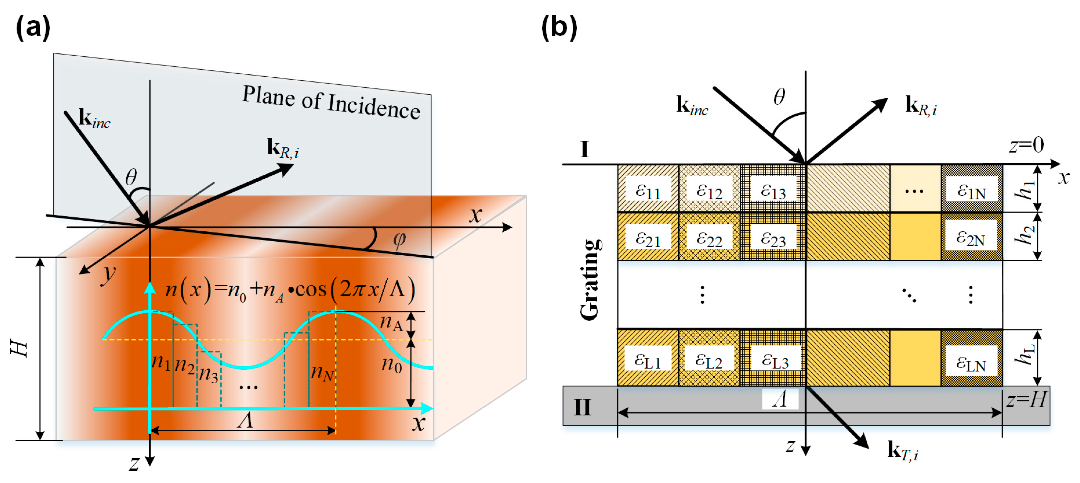
Different to common grating structures consists of ridge and groove that are typically made of two different materials (such as air and grating material), the volume grating is essentially a specific distribution of refractive indices in the material, which can be depicted as Figure 1a. The fundamental principle of such distribution formation is based on the photoinduced property changes like photopolymerization induced diffusion, or ultraviolet radiation and thermal development, giving rise to expected refractive index distribution in the recording material, such as polymer-nanoparticle composites as well as PTR glasses, etc. As in a polymer-nanoparticle system, the photo-active monomer consumption occurs in bright regions during holography because of photopolymerization, which results in the movement of monomers towards the bright regions. Consequently, the nanoparticles will be squeezed into the dark regions due to the chemical potential effects. As a result, a sinusoidal refractive index distribution as shown in Figure 1a is expected in the formed polymer nanocomposite. In order to accurately describe such a system, a distributed dielectric constant-based RCWA is proposed as the forward model for volume grating characterization.
2.1. Distributed Dielectric Constant-Based RCWA
For a volume grating whose refractive index distributed in the volume grating can be defined by an arbitrary periodic spatial function n(x) as shown Figure 1a, a RCWA model based on a distributed refractive index model can be discretized as Figure 1b. The geometric domain is divided into three regions, i.e. region I, II and the grating region, and the coordinate system is defined as shown in Figure 1. Angle of incident θ and angle of azimuth φ are defined as shown in Figure 1a as well. If a specific function of refractive index distribution can be predetermined, such as the sinusoidal distribution shown in Figure 1a, the material optical properties can be quantified by some parameters, such as the pitch Λ, the height of grating region H, the initial refractive index n0, and the amplitude of the maximum refractive index variation nA. Regardless of magnetic material, the relationship between refractive index n and relative dielectric constant ε (i.e. permittivity) is that ε = n2.
At first, the dielectric material in a period can be uniformly discretized into N units along x axis. Without losing generality, supposing the distribution can be described by a sinusoidal function, the refractive indices at an arbitrary position x can be achieved using interpolation. At the same time, if the optical property variates along z direction, a commonly used layer-by-layer discretization along z axis can be carried out as well. As shown in Figure 1b, the grating region is sliced into L layers in z direction and N units in x direction. Then, the x-dependent relative dielectric constant at l-th layer can be expanded as Fourier series
where εl,g is the g-th component of the Fourier expansion, which can be obtained as
where N is the number of units in one period. In the same way, the reciprocal of dielectric constant can be expanded as
where
The electrical field expressions of region I (z < 0) and II (z > H) can be achieved as Equations (5) and (6) by Rayleigh expansion
where Einc is normalized incident electrical field; H is total height of the volume grating; Ri is the amplitude of i-th diffractive wave; Ti is the amplitude of i-th transmit wave; r is the position vector of an arbitrary point on the plane wave front; and kR,i is the wave vector of i-th transmit wave.
According to Floquet theorem, the following conditions should be satisfied,
where i is the diffraction order, kρz,i is z component of the wave vector.
In the grating region (0 < z < H), the electric field El and magnetic field Hl can be written as Floquet-Fourier series as
where Sl,i(z) and Ul,i(z) are the amplitudes of the electric and magnetic fields of the l-th layer in the grating region. In the grating region, the electric and magnetic fields satisfy the Maxwell equations
where k0 is the wave number in the free space, given by k0 = 2π/λ0 and λ0 is the wavelength of the incident wave in free space; ε0 and μ0 are the electric permittivity and magnetic permeability in the free space and
Then submit Equations (10) and (11) to Maxwell equations Equations (12) and (13), the coupled wave equation in matrix form can be achieved as
where Kx and Ky are diagonal matrices, whose diagonal elements are kxi/k0 and kyi/k0; I is identity matrix with the same dimension of K. El-tp is the Toeplitz matrix consists of the Fourier coefficients of the relative dielectric constant at the l-th layer. Fl is the Toeplitz matrix corresponding to the reciprocal of the relative dielectric constant.
Combined with the boundary conditions and enhanced transmit matrix, the distribution of the electric field R and magnetic field T can be achieved by solving Equation (15). Further, the reflected and transmit electric fields of s- and p- polarized light can be achieved. If the transmission is considered, the amplitudes of the electric fields and the components of Jones matrix can be expressed as
And then, Mueller matrix can be calculated as
where
2.2. Inverse Problem Solving
It is insufficient to successfully obtain the measurands only with the Mueller matrices measured by MME and the Mueller matrices calculated using the forward model. An inverse problem solving process needs to be applied to find out the appropriated values for the measurands, which are able to fit the measured Mueller matrices with minimum MSE. A weighted least-squares regression analysis method (Levenberg–Marquardt algorithm) [36] is performed and the weighted mean square error function is defined as
where q stands for the q-th spectral point in Q spectral points in total, subscript indices u and v represent all the Mueller matrix elements normalized to m11 except m11, P is the measurands number, muv,q with superscript meas and calc denote the measured and calculated Mueller matrix elements, respectively, and σ(muv,q) is the estimated standard deviation associated with muv,q.
In this work, the measurands could be the parameters need to be determined in refractive index distribution function, the geometric parameters of the volume grating samples, the measurement configuration conditions such as θ and φ, and the thickness H.
3. Simulation
In order to demonstrate the generality and validity of the proposed method, a series of volume grating measurements are simulated, with different dielectric constant distribution functions. Without losing generality, three typical distribution functions such as periodic binary distribution, periodic linear distribution, as well as continuous sinusoidal distribution are selected. These functions are selected because most of the complex functions can be easily assembled by the linear combinations of these simple functions. For the convenience of comparing the effects of function type on the Mueller matrix spectra, the nominal parameters of sample setting and measurement configuration are shared. The angle of incidence θ is fixed as 25°, and the angle of azimuth φ is set as 20°. The substrates are glasses. The pitch of the dielectric distribution Λ is fix as 800 nm. For each test case of different function type, two thickness settings H are examined—3 μm and 5 μm, respectively. Considering the pitch Λ can be usually well controlled by the process of grating fabrication, we fixed it as a constant. Since the thickness H, angle of incidence θ, and the angle of azimuth φ are easily varied parameters, we need reconstruct these parameters in the fitting process.
The general procedure of the simulation can be divided into three steps. At first, according to the trues values of parameters, the theoretical Mueller matrices will be calculated. Then, random errors with signal-noise-ratio SNR = 10000 will be injected into the theoretical Mueller matrices to generate a set of measured Mueller matrices. At last, by a regression started with the initial values of parameters will be carried with the objective to best fit the measured Mueller matrices. When the optimal solution is achieved, we achieved the measured values of these parameters as well as corresponding fitted Mueller matrices.
To avoid the unphysical refractive index spectra, we quoted the correlations between the refractive index and nanoparticles weight fractions ω reported in Ref. [31], so that the appropriate refractive index curve can be selected according to the value of nanoparticles weight fraction. Then, the dielectric constant distribution function can be represented by the distribution function of the nanoparticle concentration.
3.1. Periodic Binary Distribution
In the first case, binary distribution defined by Equation (24) is used.
where ωa and ωb represent different nanoparticle concentration at different position in one pitch. f is the duty cycle of such a binary grating, which is set as 0.5 in our simulation.
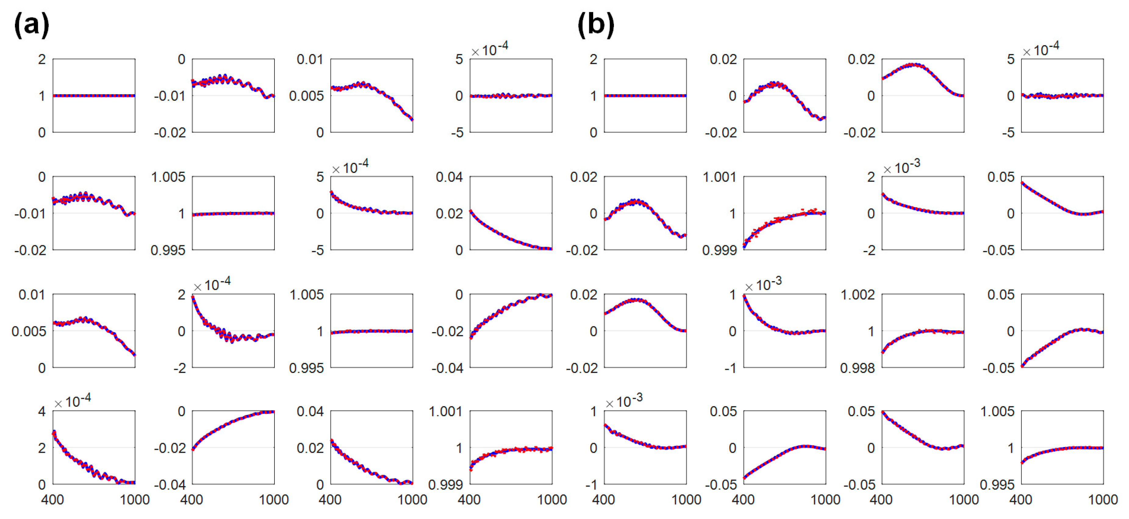
In this case, the parameters ωa and ωb are measurands we need to determine. As mentioned in the previous paragraph, H, θ, and φ are the parameters needs to be verified. The measured and fitted Mueller matrix spectra are shown in Figure 2, and the corresponding parameters are listed in Table 1.
As shown in Figure 2, although random noise has been injected into the “measured” Mueller matrices, the fitting is good. In Figure 2a,b, nonzero Mueller matrix elements in the off-diagonal elements are observed, clearly showing the anisotropy of the samples. As shown in Table 1, although the initial values of measurands ωa and ωb are given with large relative deviations to their true value, the measured values converge to their true values, which demonstrate the accuracy and robustness of the proposed method. Although the setting parameters H, θ, and φ are fitted with the same algorithm, their measured values vary in a quite small range and converge to their true values as well.
3.2. Periodic Linear Distribution
In the second test case, the fidelity of the proposed method for a periodic linear dielectric constant distribution will be examined. The distribution function is defined as
where ωb and ωk represent the intercept and the slope of the linear relationship in one pitch, respectively.
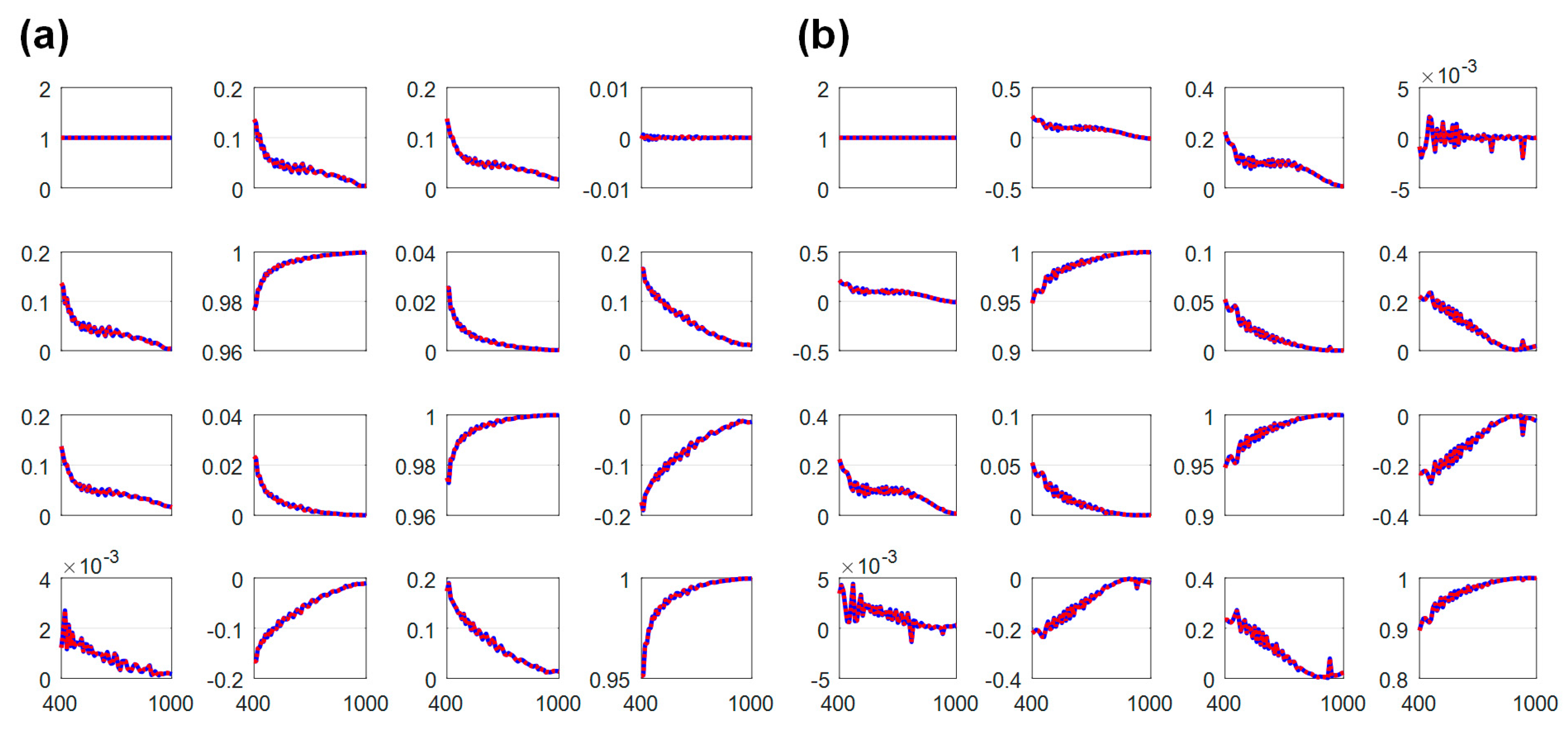
In this case, the parameters ωb and ωk are measurands we need to determine. Due to the same reason, H, θ, and φ are the parameters needs to be verified. The measured and fitted Mueller matrix spectra are shown in Figure 3, and the corresponding parameters are listed in Table 2.
Good-fitting results have been achieved as well, as shown in Figure 3. It is worth to note that the anisotropy encoded in the Mueller matrix spectra shown in Figure 3 are much more significant than the observations from Figure 2. This is because in the second case, the dielectric constant distributed in one pitch is not symmetric. The results list in Table 2 show the accuracy of the proposed method when the local optical constants are linear to the position.
3.3. Continuous Sinusoidal Distribution
In the last case study, we studied the possibility of determining a continuous dielectric constant distribution using the proposed method, because in most of the existing volume holographic gratings, the dielectric constants are considered sinusoidally distributed. The distribution function is defined as
where ω0 and ωA represent the average value and variation amplitude of nanoparticle concentration in one pitch, respectively.
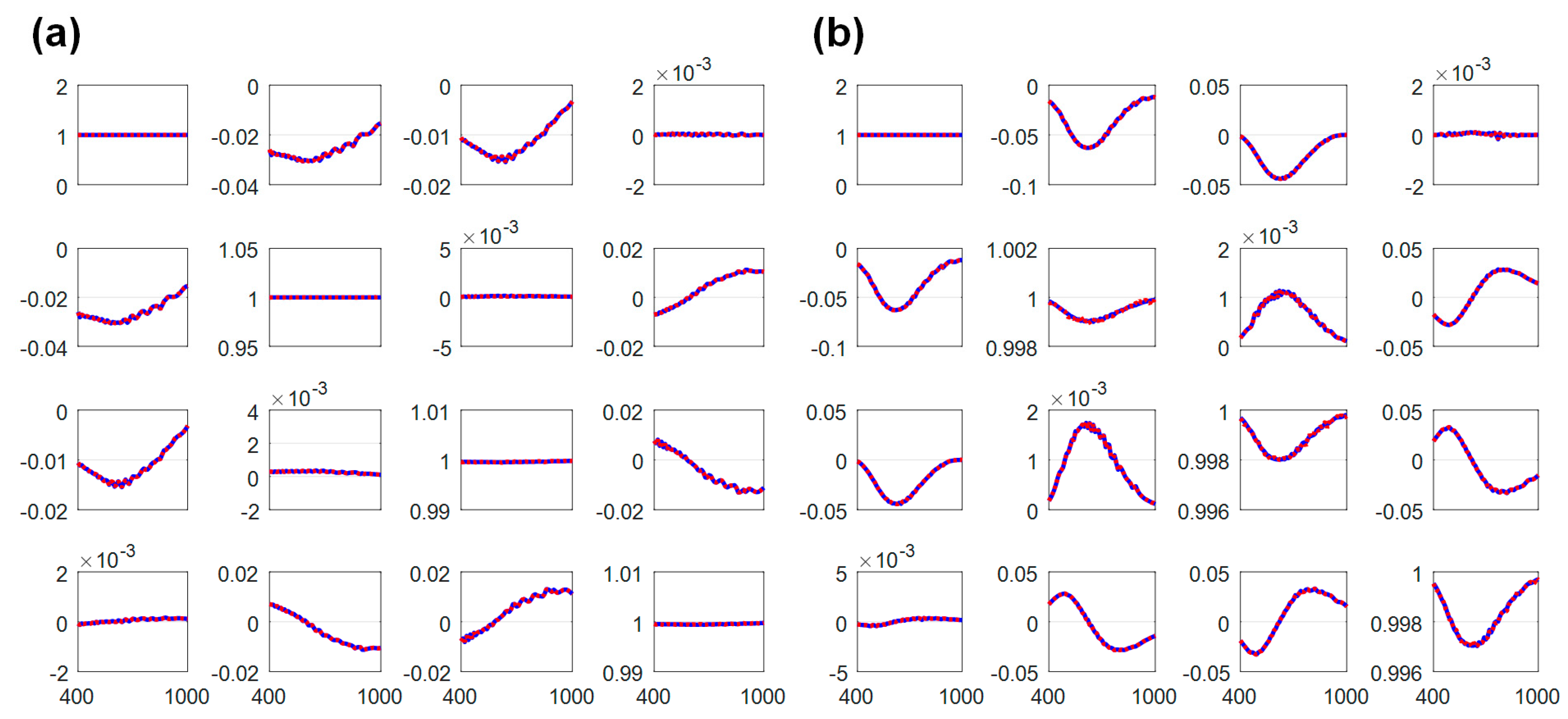
In this case, the parameters ω0 and ωA are measurands we need to determine. H, θ, and φ are reconstructed as well. The measured and fitted Mueller matrix spectra are shown in Figure 4, and the corresponding parameters are listed in Table 3.
Since the nanoparticle distribution in one pitch is symmetric again, the achieved anisotropy in the spectrum is not as significant as in the second case, where the values of the off-diagonal elements shown in Figure 4 are at the similar level as in Figure 2. If further attention is paid to the results list in Table 3, a significant improvement on the accuracy can be observed comparing to the precious two cases. It may be attributed to the less singular points for the case of a continuous distribution, which decreases the numerical errors.
The above simulations demonstrate the feasibility, effectiveness, robustness of the proposed method. It is worth to point out, more complex distribution function with more parameters need to be determined will not noticeably degrade the performance of the proposed method, since the number of wavelength points in the spectrum usually is enough for obtaining the solution. If we compare the Mueller matrix spectra reported in Figure 3, Figure 4 and Figure 5, significant differences can be distinguished, although the important parameters such as thickness, pitch, angle of incidence and azimuth, even similar interval of the refractive index changes are shared. Such high sensitivity can be used to verify the distribution function type selection, i.e., an inappropriate selection of function type is highly possible to result in the failure of regression.
4. Experiment
4.1. Volume Gratings Preparation
The volume gratings were prepared following the procedures introduces in our previous work [31]. The ZnS nanoparticles are about 5 nm in diameter, and were synthesized using pot reaction in oil bath followed by a purifying process [23,31]. Then the nanoparticles were dried in vacuum at room temperature for 2 hours. Homogeneous holographic mixtures were prepared by ultrasonication at 30 °C for 50 min with the concentration of ZnS nanoparticles as 22.6 vol% using the recipe given in [31].
To form the holographic gratings, the mixtures were inject into the cavity formed by two parallel glasses, and the thickness of the sample is controlled by the silica spacers with a diameter of ~ 8 μm. Volume gratings were recorded in the cell by two separate 442 nm He-Cd laser beams with equal intensity of 5 mW/cm2 irradiating on the cells to form a sinusoidal hologram with period of 800 nm [23,31]. Different samples were prepared by varying the duration of the irradiation of 5 s, 10 s, 15 s, 20 s, 25 s, 30 s, 35 s, and 40 s respectively. Postcure in UV with intensity of 20 mW/cm2 for 10 minutes was implemented at last to fix the grating structures.
4.2. Experimental Setup
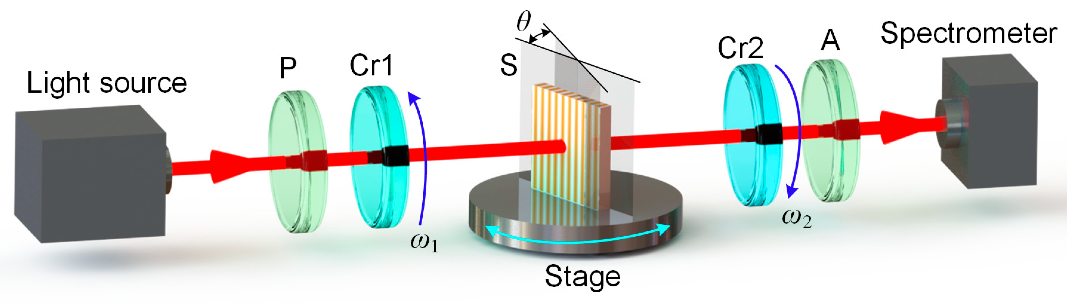
A Mueller matrix ellipsometer (ME-L ellipsometer, Wuhan Eoptics Technology Co., China) [37] will be used to measure the volume gratings. The MME has a dual rotating compensator configuration, whose layout in order of light propagation is shown in Figure 5, where P and A are the polarizer and analyzer, respectively; Cr1 and Cr2 refer to the first and second rotating compensators who are rotating with a fixed ratio of angular velocity; and S represents the holographic grating. With this instrument, the 16 Mueller matrix elements can be obtained in a single measurement. The spectral range of the instrument covers from 200 to 1000 nm. Since the light reflections from the glass surface and the sample are difficult to be differentiated by the detector in reflection mode, the transmission mode, i.e. straight through mode, was selected in our experiments. The samples are placed on the stage as shown in Figure 5. When the sample is rotated around the direction of light propagation, different azimuthal angle can be achieved. If the stage is rotated, the incident angle θ can be arbitrary selected.
4.3. Measurement Results and Discussions
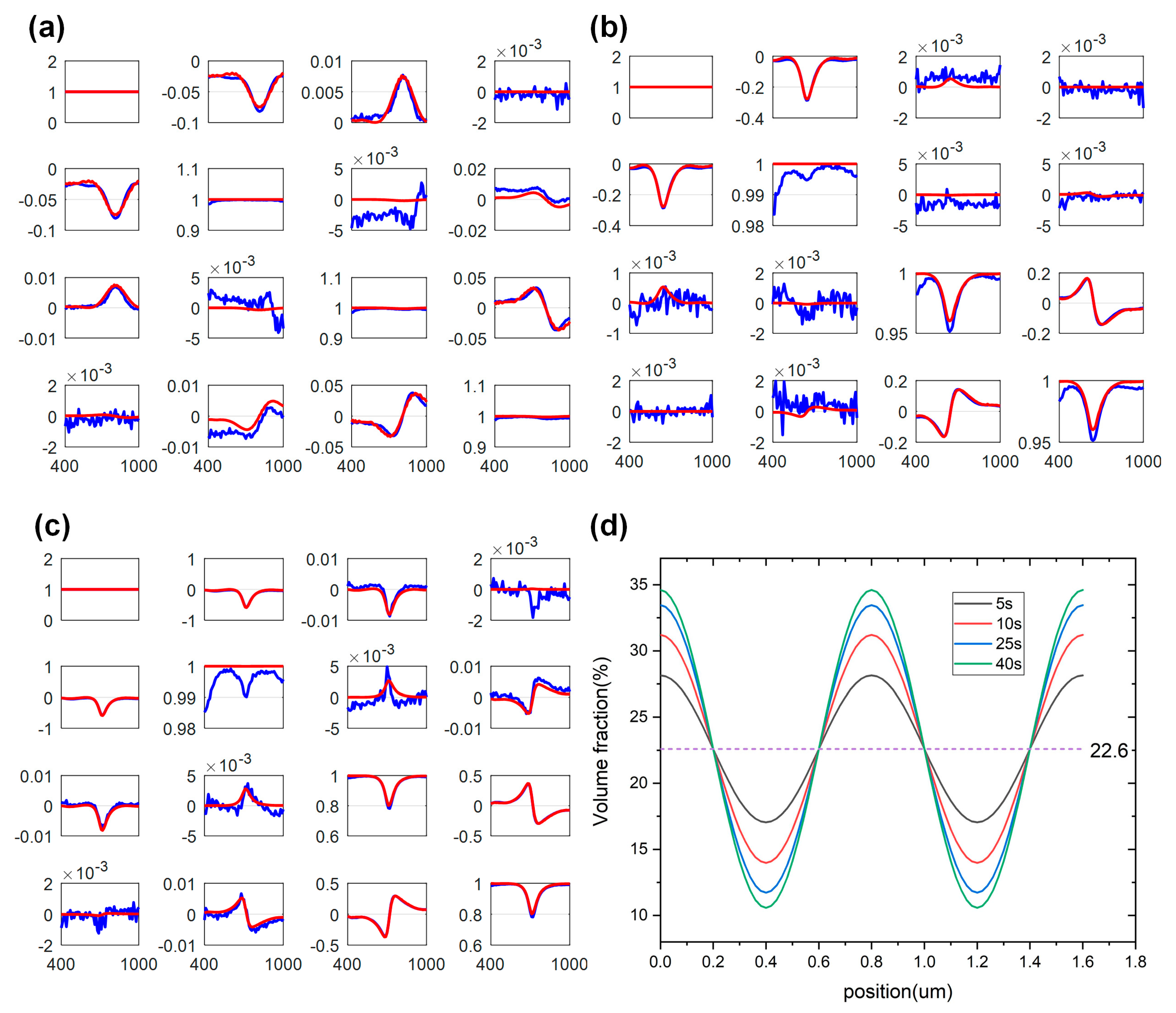
Measurement experiments are carried out on the volume holographic gratings prepared in Section 4.1. The angle of incidence θ for the probing light was fixed at approximate 25°. Since the manual manipulation cannot guarantee the exact value of angle of incidence, we set it as a measurand with an initial value of 25°. The azimuthal angle φ was set as 0°, which indicates the incident plane is perpendicular to the gratings. In this case, the off-diagonal elements in the measured Mueller matrices should be zeros, which can be applied to check the azimuthal angle settings in measurements. Same as angle of incidence, the azimuthal angle was set as a measurand with initial value of 0° to avoid the error introduced by manual manipulation. In analysis, the spectral range was from 400 to 1000 nm with an increment of 5 nm, and the distributed dielectric constant model based RCWA proposed in Section 2.1 was used to calculate the Mueller matrices. The distributed refractive index is assumed sinusoidal, which is defined as n(x) shown in Figure 1a. The number of retained orders in the truncated Fourier series was 12. Since the preliminary study [31] on the sample revealed that no significant refractive index variation along z direction had been observed because both the nanoparticles and the polymers are not absorbing materials, we set the layer number L to be 1 to improve the calculation efficiency and the measurement accuracy. In this case, the amplitude of refractive index curve nA, and the thickness of samples were measured simultaneously. Since the linear correlations between the refractive index and ZnS nanoparticles volume fraction have been achieved in our previous work [31], the distributed refractive indices can be directly converted into the volume fractions distributions. Figure 6 shows the comparison of calculated and measured Mueller matrix spectra when recording time t = 5 s, 10 s, and 40 s, as well as the achieved spatial volume fraction distributions corresponding to t = 5 s, 10 s, 25 s, and 40 s in the nanocomposite. More detailed measurement results including amplitude of concentration variation CA, thickness of samples H, the angle of incidence θ, the angle of azimuth φ, as well as the MSE of fitting are listed in Table 4. It is worth to point out that the pitch of the volume holographic grating is assumed 800 nm and the local nanoparticle concentration is ideally sinusoidally distributed.
As shown in Figure 6a–c, the measured Mueller matrix fits well with the calculated matrix. All the Mueller matrices have similar characteristics, which indicates that the formed volume gratings are consistent. If some of the specific Mueller matrix elements such as m12 are selected for a further analysis, the depth of the dip become larger, which indicates that the characteristics of Bragg grating become more and more obvious. This is rational because with the increase of the recording time, the sinusoidal distribution of the refractive index is more obvious. Such a phenomenon is more intuitively shown in Figure 6d. It can be clearly observed in Figure 6d that the volume fractions in the dark regions are increasing, while the volume fractions in the bright regions are decreasing, with the process of holographic recording. Since the nominal azimuthal angle is selected as 0°, the Mueller matrix elements observed in the off-diagonal blocks are close to 0. If we correlate the results shown in Figure 6a–c with φ reported in Table 4, the relative lager oscillations observed in Figure 6a can be attributed to the azimuthal angle setting error. Since the RIM is much larger when recording time t is 40s, even though the reconstructed azimuthal angle is as small as 0.3869°, relative more significant anisotropy, i.e. nonzero off-diagonal elements, can be observed.
In order to further demonstrate the fidelity of the proposed method, we further investigated the time-dependent volume fraction changes during holography. With the benefit of the distribution function of the refractive index, the spatiotemporal concentration function of ZnS nanoparticles expressed in terms of position x and time t, C(x, t) defined as Equation (24) [23] can be fitted directly.
where Cmax and C0 are the maximum and average nanoparticles concentration, respectively. The fitted curve can be achieved as shown in Figure 7.
The apparent diffusion coefficient, Da, achieved from the curve fitting is 2.18×10⁻¹⁵ m2 s−1, which agree to the previous results 2.0×10⁻¹⁵ m2 s−1 we reported. Such an apparent diffusion coefficient achieved using a different model exhibits again that the apparent diffusion coefficient is 3 orders lower than the initial diffusion coefficient (3.4 × 10⁻¹² m2 s−1) predicted by the Stokes–Einstein diffusion equation, which has been interpreted using the rapid increase of the mixture viscosity during polymerization [31].
5. Conclusions
In order to appropriately reflect the distribution of refractive indices in the volume grating so that the grating can be accurately characterized, a distributed dielectric constant-based RCWA is proposed as a forward model that can be used for ellipsometry. A set of measurement experiments is carried out on the volume gratings recorded in the composite of polymer and 5-nm ZnS nanoparticles with a different holographic recording time for demonstration. With the proposed model, parameters of the spatial refractive index distribution curve of a volume grating can be quantified, which also enables the quantitative determination of the spatiotemporal concentration function. Good agreement of the experimental results to the values we previously reported demonstrates the fidelity of the proposed method.
Author Contributions
Conceptualization, H.J.; methodology, H.J.; software, Z.M.; validation, H.J., and Z.M.; formal analysis, H.J., and Z.M.; writing—original draft preparation, H.J.; writing—review and editing, H.G., X.C., and S.L.; supervision, H.J. and S.L.; project administration, H.J. and S.L.; funding acquisition, H.J. and S.L.
Funding
This research was funded by the National Natural Science Foundation of China (Grant Nos. 51575214, 51525502, 51727809, and 51805193), the National Key Research and Development Plan (Grant No. 2017YFF0204705); the National Science and Technology Major Project of China (Grant No. 2017ZX02101006-004), and the Natural Science Foundation of Hubei Province of China (Grant Nos. 2018CFA057 and 2018CFB559).
Conflicts of Interest
The authors declare no conflicts of interest.
References
- Heifetz, A.; Shen, J.T.; Lee, J.K.; Tripathi, R.; Shahriar, M.S. Translation-invariant object recognition system using an optical correlator and a super-parallel holographic RAM. Opt. Eng. 2006, 45, 025201. [Google Scholar] [CrossRef]
- Fernandez, R.; Gallego, S.; Marquez, A.; Frances, J.; Navarro, V.; Pascual, I. Diffractive lenses recorded in absorbent photopolymers. Opt. Express 2016, 24, 1559–1572. [Google Scholar] [CrossRef] [PubMed] [Green Version]
- Iazikov, D.; Greiner, C.M.; Mossberg, T.W. Integrated holographic filters for flat passband optical multiplexers. Opt. Express 2006, 14, 3497–3502. [Google Scholar] [CrossRef] [PubMed]
- Aksenova, K.A.; Angervaks, A.E.; Shcheulin, A.S.; Ryskin, A.I. Holographic characteristics of calcium fluoride crystals in the IR region. J. Opt. Technol. 2015, 82, 760. [Google Scholar] [CrossRef]
- Mikutis, M.; Kudrius, T.; Šlekys, G.; Paipulas, D.; Juodkazis, S. High 90% efficiency Bragg gratings formed in fused silica by femtosecond Gauss-Bessel laser beams. Opt. Mater. Express 2013, 3, 1862. [Google Scholar] [CrossRef]
- Zhang, Y.J.; Zhang, G.D.; Chen, C.L.; Stoian, R.; Cheng, G.H. Transmission volume phase holographic gratings in photo-thermo-refractive glass written with femtosecond laser Bessel beams. Opt. Mater. Express 2016, 6, 3491. [Google Scholar] [CrossRef]
- Lumeau, J.; Glebov, L. Effect of the refractive index change kinetics of photosensitive materials on the diffraction efficiency of reflecting Bragg gratings. Appl. Opt. 2013, 52, 3993–3997. [Google Scholar] [CrossRef]
- Dmitry, K.; Sergei, I.; Victoria, K.; Martti, S.; Yuri, S.; Nikolay, N. Thermal stability of volume bragg gratings in chloride photo-thermo-refractive glass after femtosecond laser bleaching. Opt. Lett. 2018, 43, 1083. [Google Scholar]
- Chen, P.; He, D.; Jin, Y.; Chen, J.; Zhao, J.; Xu, J. Method for precise evaluation of refractive index modulation amplitude inside the volume bragg grating recorded in photo-thermo-refractive glass. Opt. Express 2018, 26, 157. [Google Scholar] [CrossRef]
- Guo, J.; Gleeson, M.R.; Sheridan, J.T. A review of the optimisation of photopolymer materials for holographic data storage. Phys. Res. Int. 2012, 2012, 803439. [Google Scholar] [CrossRef]
- Sabel, T.; Zschocher, M. Transition of refractive index contrast in course of grating growth. Sci. Rep. 2013, 3, 2552. [Google Scholar] [CrossRef]
- Ji, R.; Fu, S.; Zhang, X.; Han, X.; Liu, S.; Wang, X.; Liu, Y. Fluorescent holographic fringes with a surface relief structure based on merocyanine aggregation driven by blue-violet laser. Sci. Rep. 2018, 8, 3818. [Google Scholar] [CrossRef] [PubMed]
- De Sio, L.; Lloyd, P.F.; Tabiryan, N.V.; Bunning, T.J. Hidden gratings in holographic liquid crystal polymer-dispersed liquid crystal films. ACS Appl. Mater. Interfaces 2018, 10, 13107–13112. [Google Scholar] [CrossRef] [PubMed]
- Ni, M.; Peng, H.; Xie, X. Structure regulation and performance of holographic polymer dispersed liquid crystals. Acta Polym. Sin. 2017, 48, 1557–1573. [Google Scholar]
- Vaia, R.A.; Dennis, C.L.; Natarajan, L.V.; Tondiglia, V.P.; Tomlin, D.W.; Bunning, T.J. One-step, micrometer-scale organization of nano- and mesoparticles using holographic photopolymerization: A generic technique. Adv. Mater. 2001, 13, 1570–1574. [Google Scholar] [CrossRef]
- Garnweitner, G.; Goldenberg, L.M.; Sakhno, O.V.; Antonietti, M.; Niederberger, M.; Stumpe, J. Large-scale synthesis of organophilic zirconia nanoparticles and their application in organic-inorganic nanocomposites for efficient volume holography. Small 2007, 3, 1626–1632. [Google Scholar] [CrossRef]
- Sanchez, C.; Escuti, M.J.; van Heesch, C.C.; Bastiaansen, W.M.; Broer, D.J.; Loos, J.; Nussbaumer, R. TiO2 nanoparticle-photopolymer holographic recording. Adv. Funct. Mater. 2005, 15, 1623–1629. [Google Scholar] [CrossRef]
- Suzuki, N.; Tomita, Y.; Kojima, T. Holographic recording in TiO2 nanoparticle-dispersed methacrylate photopolymer films. Appl. Phys. Lett. 2002, 81, 4121–4123. [Google Scholar] [CrossRef]
- Smirnova, T.N.; Sakhno, O.V.; Yezhov, P.V.; Kokhtych, L.M.; Goldenberg, L.M.; Stumpe, J. Amplified spontaneous emission in polymer-CdSe/ZnS-nanocrystal DFB structures produced by the holographic method. Nanotechnology 2009, 20, 245707. [Google Scholar] [CrossRef] [PubMed]
- Ostrowski, A.M.; Naydenova, I.; Toal, V. Light-induced redistribution of Si-MFI zeolite nanoparticles in acrylamide-based photopolymer holographic gratings. J. Opt. A Pure Appl. Opt. 2009, 11, 034004. [Google Scholar] [CrossRef]
- Berberova, N.; Daskalova, D.; Strijkova, V.; Kostadinova, D.; Nazarova, D.; Nedelchev, L.; Stoykova, E.; Marinova, V.; Chi, C.; Lin, S. Polarization holographic recording in thin films of pure azopolymer and azopolymer based hybrid materials. Opt. Mater. 2017, 64, 212–216. [Google Scholar] [CrossRef]
- Lü, C.; Cheng, Y.; Liu, Y.; Liu, F.; Yang, B. A facile route to ZnS–polymer nanocomposite optical materials with high nanophase content via γ-ray irradiation initiated bulk polymerization. Adv. Mater. 2006, 18, 1188–1192. [Google Scholar] [CrossRef]
- Ni, M.; Peng, H.; Liao, Y.; Yang, Z.; Xue, Z.; Xie, X. 3D image storage in photopolymer/ZnS nanocomposites tailored by “photoinitibitor”. Macromolecules 2015, 48, 2958–2966. [Google Scholar] [CrossRef]
- Peng, H.; Bi, S.; Ni, M.; Xie, X.; Liao, Y.; Zhou, X.; Xue, Z.; Zhu, J.; Wei, Y.; Bowman, C.N.; et al. Monochromatic visible light “photoinitibitor”: Janus-faced initiation and inhibition for storage of colored 3D images. J. Am. Chem. Soc. 2014, 136, 8855–8858. [Google Scholar] [CrossRef] [PubMed]
- Sabel, T.; Zschocher, M. Imaging of Volume Phase Gratings in a Photosensitive Polymer, Recorded in Transmission and Reflection Geometry. Appl. Sci. 2014, 4, 19–27. [Google Scholar] [CrossRef] [Green Version]
- Juhl, A.T.; Busbee, J.D.; Koval, J.J.; Natarajan, L.V.; Tondiglia, V.P.; Vaia, R.A.; Bunning, T.J.; Braun, P.V. Holographically directed assembly of polymer nanocomposites. ACS Nano 2010, 4, 5953–5961. [Google Scholar] [CrossRef]
- Óscar, M.; Calvo, M.L.; Rodrigo, J.A.; Cheben, P.; Monte, F.D. Diffusion study in tailored gratings recorded in photopolymer glass with high refractive index species. Appl. Phys. Lett. 2007, 91, 141115. [Google Scholar] [Green Version]
- Klepp, J.; Tomita, Y.; Pruner, C.; Kohlbrecher, J.; Fally, M. Three-port beam splitter for cold neutrons using holographic nanoparticle-polymer composite diffraction gratings. Appl. Phys. Lett. 2012, 101, 154104. [Google Scholar] [CrossRef]
- Goldenberg, L.M.; Sakhno, O.V.; Smimova, T.N.; Helliwell, P.; Chechik, V.; Stumpe, J. Holographic composites with gold nanoparticles: Nanoparticles promote polymer segregation. Chem. Mater. 2008, 20, 4619–4627. [Google Scholar] [CrossRef]
- Butcher, H.L.; MacLachlan, D.G.; Lee, D.; Brownsword, R.A.; Thomson, R.R.; Weidmann, D. Mid-infrared volume diffraction gratings in IG2 chalcogenide glass: Fabrication, characterization, and theoretical verification. Proc. SPIE 2018, 10528, 105280R. [Google Scholar]
- Jiang, H.; Peng, H.; Chen, G.; Gu, H.; Chen, X.; Liao, Y.; Liu, S.; Xie, X. Nondestructive investigation on the nanocomposite ordering upon holography using Mueller matrix ellipsometry. Eur. Polym. J. 2019, 110, 123–129. [Google Scholar] [CrossRef]
- Mokhov, S.; Ott, D.; Smirnov, V.; Divliansky, I.; Zeldovich, B.; Glebov, L. Moiré apodized reflective volume Bragg grating. Opt. Eng. 2018, 57, 037106. [Google Scholar] [CrossRef]
- Li, H.; Qi, Y.; Guo, C.; Malallah, R.; Sheridan, J.T. Holographic characterization of diffraction grating modulation in photopolymers. Appl. Opt. 2018, 57, E107–E117. [Google Scholar] [CrossRef] [PubMed]
- Li, C.; Cao, L.; He, Q.; Jin, G. Holographic kinetics for mixed volume gratings in gold nanoparticles doped photopolymer. Opt. Express 2018, 22, 5017–5028. [Google Scholar] [CrossRef] [PubMed]
- Moharam, M.G.; Gaylord, T.K. Rigorous coupled-wave analysis of planar-grating diffraction. J. Opt. Soc. Am. 1981, 71, 811–818. [Google Scholar] [CrossRef]
- Press, W.H.; Teukolsky, S.A.; Vetterling, W.T.; Flannery, B.P. Numerical Recipes: The Art of Scientific Computing; Cambridge University Press: Cambridge, UK, 2007. [Google Scholar]
- Liu, S.; Chen, X.; Zhang, C. Development of a broadband Mueller matrix ellipsometer as a powerful tool for nanostructure metrology. Thin Solid Films 2015, 584, 176–185. [Google Scholar] [CrossRef]
Figure 1.
Scheme of the (a) spatial refractive index distribution in a volume grating; and (b) the corresponding distributed dielectric constant model used for rigorous coupled-wave analysis.
Figure 1.
Scheme of the (a) spatial refractive index distribution in a volume grating; and (b) the corresponding distributed dielectric constant model used for rigorous coupled-wave analysis.

Figure 2.
Measured Mueller matrix spectra (blue) and fitted Mueller matrix spectra (red) for the volume gratings whose dielectric constant is a periodic binary distribution, with thicknesses of (a) 3 μm and (b) 5 μm, respectively.
Figure 2.
Measured Mueller matrix spectra (blue) and fitted Mueller matrix spectra (red) for the volume gratings whose dielectric constant is a periodic binary distribution, with thicknesses of (a) 3 μm and (b) 5 μm, respectively.

Figure 3.
Measured Mueller matrix spectra (blue) and fitted Mueller matrix spectra (red) for the volume gratings whose dielectric constant is a periodic linear distribution, with thicknesses of (a) 3 μm and (b) 5 μm, respectively.
Figure 3.
Measured Mueller matrix spectra (blue) and fitted Mueller matrix spectra (red) for the volume gratings whose dielectric constant is a periodic linear distribution, with thicknesses of (a) 3 μm and (b) 5 μm, respectively.

Figure 4.
Measured Mueller matrix spectra (blue) and fitted Mueller matrix spectra (red) for the volume gratings whose dielectric constant is a continuous sinusoidal distribution, with thicknesses of (a) 3 μm and (b) 5 μm, respectively.
Figure 4.
Measured Mueller matrix spectra (blue) and fitted Mueller matrix spectra (red) for the volume gratings whose dielectric constant is a continuous sinusoidal distribution, with thicknesses of (a) 3 μm and (b) 5 μm, respectively.

Figure 5.
Scheme of the experimental setup based on a dual rotating-compensator Mueller matrix ellipsometer (MME) in the transmission mode.
Figure 5.
Scheme of the experimental setup based on a dual rotating-compensator Mueller matrix ellipsometer (MME) in the transmission mode.

Figure 6.
Results of calculated (red) and measured (blue) Mueller matrix spectra in the transmission mode when recording time (a) t = 5s; (b) t = 10s; (c) t = 40s; and (d) measured spatial refractive index distribution curve of a volume grating at different exposure time.
Figure 6.
Results of calculated (red) and measured (blue) Mueller matrix spectra in the transmission mode when recording time (a) t = 5s; (b) t = 10s; (c) t = 40s; and (d) measured spatial refractive index distribution curve of a volume grating at different exposure time.

Figure 7.
Fitting result of spatiotemporal concentration of ZnS nanoparticles.


Table 1.
Simulation results of case 1.
| H (μm) | ωa | ωb | H | θ | φ | |
|---|---|---|---|---|---|---|
| 3 | Initial value | 0.16 | 0.38 | 3.1 | 23.5 | 18 |
| Measured value | 0.28 | 0.44 | 2.99 | 24.79 | 19.14 | |
| True values | 0.26 | 0.42 | 3 | 25 | 20 | |
| 5 | Initial value | 0.16 | 0.38 | 5.1 | 23.5 | 18 |
| Measured value | 0.29 | 0.45 | 4.98 | 24.92 | 19.98 | |
| True values | 0.26 | 0.42 | 5 | 25 | 20 |
Table 2.
Simulation results of case 2.
| H (μm) | ωb | ωk | H | θ | φ | |
|---|---|---|---|---|---|---|
| 3 | Initial value | 0.18 | 1.1 | 2.8 | 23.5 | 18 |
| Measured value | 0.20 | 1.02 | 2.85 | 23.56 | 18.97 | |
| True values | 0.2 | 1 | 3 | 25 | 20 | |
| 5 | Initial value | 0.18 | 1.1 | 4.8 | 23.5 | 18 |
| Measured value | 0.21 | 1.00 | 4.98 | 23.75 | 20.01 | |
| True values | 0.2 | 1 | 5 | 25 | 20 |
Table 3.
Simulation results of case 3.
| H (μm) | ω0 | ωA | H | θ | φ | |
|---|---|---|---|---|---|---|
| 3 | Initial value | 0.3 | 0.1 | 3.1 | 23.5 | 18 |
| Measured value | 0.36 | 0.15 | 3.00 | 25.00 | 20.00 | |
| True values | 0.36 | 0.15 | 3 | 25 | 20 | |
| 5 | Initial value | 0.34 | 0.13 | 5.1 | 23.5 | 18 |
| Measured value | 0.39 | 0.15 | 5.01 | 24.99 | 20.00 | |
| True values | 0.36 | 0.15 | 5 | 25 | 20 |
Table 4.
Measured results of volume gratings with different exposure time.
| time(s) | C0 | CA | H (μm) | θ (o) | φ (o) | MSE |
|---|---|---|---|---|---|---|
| 5 | 0.226 | 0.055 | 8.2052 | 30.5508 | −3.6431 | 4.8585 |
| 10 | 0.086 | 9.2286 | 23.8851 | −0.0558 | 4.6035 | |
| 15 | 0.108 | 8.4533 | 26.7676 | −1.22687 | 6.1378 | |
| 20 | 0.113 | 9.375 | 28.3695 | −0.7261 | 14.0584 | |
| 25 | 0.109 | 9.8429 | 25.6022 | 1.7953 | 21.8013 | |
| 30 | 0.104 | 8.2554 | 26.5644 | −2.9308 | 2.9309 | |
| 35 | 0.113 | 6.5781 | 25.2278 | −0.9119 | 6.004 | |
| 40 | 0.120 | 8.763 | 26.7677 | 0.3869 | 6.7657 |
© 2019 by the authors. Licensee MDPI, Basel, Switzerland. This article is an open access article distributed under the terms and conditions of the Creative Commons Attribution (CC BY) license (http://creativecommons.org/licenses/by/4.0/).
Share and Cite
MDPI and ACS Style
Jiang, H.; Ma, Z.; Gu, H.; Chen, X.; Liu, S. Characterization of Volume Gratings Based on Distributed Dielectric Constant Model Using Mueller Matrix Ellipsometry. Appl. Sci. 2019, 9, 698. https://doi.org/10.3390/app9040698
AMA Style
Jiang H, Ma Z, Gu H, Chen X, Liu S. Characterization of Volume Gratings Based on Distributed Dielectric Constant Model Using Mueller Matrix Ellipsometry. Applied Sciences. 2019; 9(4):698. https://doi.org/10.3390/app9040698
Chicago/Turabian StyleJiang, Hao, Zhao Ma, Honggang Gu, Xiuguo Chen, and Shiyuan Liu. 2019. "Characterization of Volume Gratings Based on Distributed Dielectric Constant Model Using Mueller Matrix Ellipsometry" Applied Sciences 9, no. 4: 698. https://doi.org/10.3390/app9040698
Note that from the first issue of 2016, this journal uses article numbers instead of page numbers. See further details here.