Suppression of the Hydrodynamic Noise Induced by the Horseshoe Vortex through Mechanical Vortex Generators

1
Acoustic Science and Technology Laboratory, Harbin Engineering University, Harbin 150001, China
2
Key Laboratory of Marine Information Acquisition and Security (Harbin Engineering University), Ministry of Industry and Information Technology or Laboratory, Harbin 150001, China
3
College of Underwater Acoustic Engineering, Harbin Engineering University, Harbin 150001, China
*
Author to whom correspondence should be addressed.
Appl. Sci. 2019, 9(4), 737; https://doi.org/10.3390/app9040737
Submission received: 26 January 2019
/
Revised: 14 February 2019
/
Accepted: 18 February 2019
/
Published: 20 February 2019
(This article belongs to the Special Issue Active and Passive Noise Control)
Abstract
:Featured Application
The proposed method can be used to reduce the hydrodynamic noise from underwater vehicles at low frequency.
Abstract
The hydrodynamic noise from the horseshoe vortex can greatly destroy the acoustic stealth of underwater vehicles at low frequency. We investigated the flow-induced noise suppression mechanism by mechanical vortex generators (VGs) on a SUBOFF model. Based on the numerical simulation, we calculated the flow field and the sound field of the three shapes of mechanical VGs: triangular, semi-circular, and trapezoidal. The triangular VGs with an angle of 30° to the flow direction achieved a better noise reduction. The optimum noise suppression is 8.93 dB, when the distance from the triangular VGs to the sail hull’s leading edge is 0.1c, where c is the chord length. The noise reduction mechanism is such that the mechanical VGs can destroy the formation of the horseshoe vortex at the origin and produce counter-rotation vortices to weaken its intensity. We created two steel models according to the simulation, and the experimental measurement was carried out in a gravity water tunnel. The measured results showed that the formation of the horseshoe vortex could be effectively inhibited by the triangular VGs. The results in our study can provide a new method for hydrodynamic noise suppression by flow control.
1. Introduction
The noise sources of a submarine can be categorized into propeller noise, hydrodynamic noise, and mechanical noise. With modern techniques available for the control of propeller noise and mechanical noise, hydrodynamic noise becomes significant, especially when the speed of the submarine is higher than 12 knots [1]. The generation mechanism of the hydrodynamic noise is as follows. First, when the fluid flows around the surface of the submarine, the turbulent fluctuation pressure produces and radiates self-noise, which is known as the flow noise. Second, the turbulent fluctuation pressure excites the elastic shell of the submarine to vibrate and radiate another noise, known as the flow-induced noise. Since the sound radiation efficiency of the flow-induced noise is much higher than that of the flow noise, the latter is usually ignored. Therefore, the hydrodynamic noise only means the flow-induced noise in some cases. Since the flow-induced noise dramatically destroys the submarine’s acoustic stealth performance, the reduction of the flow-induced noise is of great significance to enhance the submarine’s combat and survival performance [2].
The methods developed for the reduction of the submarine’s flow-induced noise are focused on the optimization of line type, active flow control, and passive flow control. In the passive flow control field, the vortex generator (VG) is a practical tool used to suppress the flow separation [3] and inhibit the vibration [4]. The inverted wing with VG highlights the flow physics of how the flow separation can be controlled by VGs [5]. Low-profile VGs have been successfully utilized by at least two other aircrafts [6]. VGs are able to redirect flow and increase lift [7], and even to mitigate shock-induced separation [8]. The supersonic VGs can also reduce flow separation near the throat [9]. A 5% drag reduction can be achieved using proper VG configurations through cumulated effects of flow reattachment [10]. However, some researchers have revealed that, although VGs are simple devices, they still generate drag [11] because stronger vortices are generated by VGs in larger dimensions, which do not necessarily lead to better flow separation control [12]. Thereafter, the micro VG was proposed [13], where shock-induced flow separation can be partially eliminated by the vortices produced from micro VGs [14]. Verma [15] has found that the increase of the control micro VG’s height appears to be favorable for closer control location, and thus the mechanism of flow control by the VG has drawn researchers’ interests.
The results of flow control by the VG were validated by experiments because the capability of numerical calculation is limited by the grid numbers. Examples include Godard’s parametric study of passive VGs using the stereo Particle Image Velocity (PIV) experiment [16], Lo’s experimental study of vane-type VGs [17], Zhang’s experimental investigation of low-profile VGs [18], and Lengani’s analyses of the experimental study on low profile VGs [19].
With the development of advanced technologies, some models have been proposed to calculate the flow field of VGs. For instance, Törnblom explored VG control of parameter variations at a low computational cost [20]. The integral boundary layer code XFOIL was used to model the effect of VGs by De Tavernier [21]. Li used the monotone integrated large-eddy simulation method to investigate the declining angles of the trailing edge of micro-ramp VGs [22]. Wang investigated the airfoil S809’s aerodynamic performance, without and with VGs, using simulations [23]. Jira´sek found that the jBAY model captured the VG arrays effect under internal and external flows [24]. Joubert investigated an OA209 airfoil with a deployable VG device through numerical simulations [25]. Yan used simulations to investigate the flow over a compression ramp, with and without a micro-ramp VG upstream [26].
On the one hand, the position of the VG is an important parameter. The 0° VG is unacceptable because it not only raises the velocity fluctuation, but it also enhances the buffeting phenomenon [27]. The VGs’ streamwise position, as well as the height and placement of the VG model, strongly affect the skin friction distribution [28]. Giepman found that the micro-ramp VG was most effective along its centerline [29]. On the other hand, the size of the VG is also believed to be a critical parameter. The vorticity from a dissymmetric micro-ramp VG is stronger than that from a standard micro-ramp VG [30]. A rod VG was proposed to enhance the stream-wise shear stresses and to effectively reduce flow separation [31]. Součková found that the rectangular vane VGs seemed to be more effective than the triangular ones [32].
The listed references are mainly focused on the improvement of the flow field by VGs, and the work is mainly done in the aviation field. In the hydrodynamic field, only Manshadi [33] found that mid-VGs could significantly reduce the cross-flow separation and the drag force, but the author did not consider the hydrodynamic noise. The utilization of a VG in underwater vehicles must be investigated in detail, especially the level change in the hydrodynamic noise. Since the physical difference between water and air is enormous, the results in the aviation field can only be considered as a reference. First, an object in the air, like an airplane, is running at high speed, at least 20 times faster than a submarine. The former encounters the problem of shock waves, while the latter encounters cavitation. The formation mechanism of the two problems is different. Second, air is a light medium, while water is a heavy medium. Therefore, the generation mechanism of aerodynamic noise and hydrodynamic noise is different, because the aerodynamic noise neglects the coupling between the shell and the air. Third, the source of aerodynamic noise is mainly from the boundary layer separation, while the boundary layer separation is only one of the hydrodynamic noise sources. Fourth, the boundary layer thickness of air is larger than that of water, and the Reynolds number in air is less than that in water. Therefore, the flow control reports on VGs in the air cannot be directly used to reduce the hydrodynamic noise.
Since VGs can be used to redirect the flow in the aerodynamic field, we proposed the idea that mechanical VGs can be applied to reduce a submarine’s flow-induced noise through the proper flow control. In this research, we placed VGs at the leading edge of the sail hull on a scaled SUBOFF model to inhibit the formation and development of the horseshoe vortex. We established the calculation process of the flow field and the sound field. The method of large eddy simulation (LES) was used to calculate the flow field. Then, the turbulent fluctuation pressure was extracted. The wavenumber–frequency spectrum method was used to estimate the sound radiation. We revealed the mechanism of mechanical VGs in rearranging the flow field and reducing the flow-induced noise. The VGs with the optimum noise reduction effect on the model were summarized and validated by experiments conducted in a water tunnel. The results from our study can provide a new way to reduce the hydrodynamic noise and enhance the acoustic stealth level of underwater vehicles, such as submarines, torpedoes, unmanned underwater vehicles (UUVs), etc.
2. The Theory of Numerical Simulation
2.1. LES Method
The flow field of the model is numerically calculated using the LES, and the turbulent fluctuation pressure is extracted from the simulation. In the theory of the LES [34], turbulent vortices are divided into two parts: the large-scale vortex and small-scale vortex. The large-scale vortex provides the major part of the turbulent energy. However, the small-scale vortex only dissipates the turbulent energy. More specifically, a filter function is established in the method, which can filter out the small-scale vortex. The large-scale vortex is introduced into the Navier–Stokes (NS) equation and then solved. The sub-grid stress terms are added to the NS equation to show the small-scale vortex’s effect on the flow field. The filtered NS equation is:
where is the sub-grid stress term, and is also called the filtered stress tensor. The dynamic sub-grid model proposed by Germano was added to yield Equation (1) as shown in [35], which can be suitably adapted into the local turbulent structure near the wall.
where is the coefficient of sub-grid eddy viscosity, is the sub-grid scale Reynolds stress, and is the strain tensor rate, which can be written as:
where is the scale of the filter, and is equivalent to the mix length. The dynamic sub-grid model needs to be continuously adjusted to suit different computational processes. The convection field needs to be filtered many times, and the results are as follows:
where is the resolved stress, and is the tensor.
2.2. Theory of Vibration and Sound Radiation by the Flow-Induced Force
When the fluid flows around the model, the shell will vibrate under the flow-induced force. Then, the noise will be radiated from the model by the flow excitation. In the theory of vibration and sound radiation from the shell under the flow-induced force, some assumptions need to be upheld, as follows.
- (1)
- The turbulent pressure field is spatially uniform and static relative to time. That is, the time–space correlation of wall pressure fluctuation only depends on the spatial distance and time interval.
- (2)
- The sound radiation from the vibration of the model is under the excitation of turbulent fluctuation pressure, while that from the turbulent fluctuation pressure itself is ignored.
- (3)
- The properties of the model are isotropic and obey the theory of elasticity.
If denotes the turbulent fluctuation pressure, which excites the shell of the model, then can be decomposed by the wavenumber–frequency spectrum:
If is the function of the wavenumber–frequency transformation and is introduced to express the response of the excitation of the infinite plate by turbulent fluctuation pressure, then the pressure at any point in the system can be shown as:
In the random fields, the time–space correlation function can be written in plural form:
where 〈 〉 denotes the average. If Equation (10) is substituted into Equations (11) and (12), then the function of the time–space correlation of the random field is obtained:
where is the density function of the wavenumber–frequency spectrum. Then,
where is the function of cross-spectrum density. Then,
To describe the pressure fluctuation of the turbulent boundary layer, the Corcos model was adopted. The function of cross-spectrum density can be acquired:
where and are two constants related to the surface roughness, is the migration wave number, and is the migration turbulence velocity. If the randomness in the direction is ignored, then,
The function of cross-spectrum density in Equation (16) is not related to , so Equation (15) can be simplified to:
If the theorem of the residue is applied,
where denotes the direct transformation of the system to the migration peak of the turbulent fluctuation pressure. The property of the sound field is similar to that of the turbulent fluctuation pressure:
Equation (20) denotes the radiation, which is generated by the shell resonance excited by turbulent pressure fluctuation.
From Equation (20), we can see that the flow-induced noise from the model is determined by the shell’s resonance mode. This theory can provide some guidelines for the numerical simulation. Since the model is of limited dimensions, the sound radiation distribution in the frequency axis is sparse in the low-frequency range, and dense in the high-frequency range. Meanwhile, the data from the fluctuation pressure sensor can be transformed by the wavenumber–frequency spectrum. Then, the sound radiation can be estimated by Equation (20). Therefore, the combination of the turbulent fluctuation pressure measurement method and the reverberation method can be used to evaluate the hydrodynamic noise from the model. The variation of turbulent fluctuation pressure can be used to evaluate the low-frequency noise reduction effect by the mechanical VGs. This can solve the problem that the reverberation method cannot measure the low-frequency hydrodynamic noise.
2.3. The Accuracy Validation of the Numerical Simulation
Based on the listed theory, we established the process of numerical simulation. The flow field was computed using the LES. The sound field was obtained by a combination of the Lighthill’s acoustic analogy with the finite element method [34]. To validate the accuracy of the calculation, we created the model according to Heatwole [36], who conducted an experimental test on the air flows around a plate with simple support. The speed of air flow was 35.8 m/s. Figure 1 shows the comparison between the test and the calculation.
There was a minor difference in the sound pressure level in the frequency range between the two results. The reason was that microphones are the practical tools with some spacing, while the points in the numerical simulation were virtual, only picked up according to the receiver’s position, as described in [36]. However, we see the trend of the sound pressure level changing with the frequency in the numerical simulation as being very similar to that in the experimental test. The total sound pressure level difference between them was only 0.6%, which can be neglected. Therefore, the established process of numerical calculation was feasible and could be used to calculate the flow-induced noise from the SUBOFF model.
3. The Description of the Model in Numerical Simulation
3.1. The Research Model
The SUBOFF is a specific model of the submarine, which was jointly proposed by Defence Advanced Research Projects Agency (DARPA) and David Taylor Research Center (DTRC). To reveal the phenomena of the horseshoe vortex, reduce the number of the grids, and to save time in numerical calculations, we neglected some parts of the submarine body in the SUBOFF model. The selected object was a whole sail hull with part of the body. Since the horseshoe vortex is generated near the leading edge of the sail hull, then developed at the bottom side of the sail hull, and dissipated at the tail of the sail hull, the flow at other parts of the SUBOFF model had no effect on the horseshoe vortex’s generation, development, and dissipation. Moreover, the noise reduction was evaluated by the comparison between the original model and the model with the mechanical VGs, that is, the noise reduction was a relative value, not an absolute value. As long as the horseshoe vortex was formed, the results were enough for the evaluation. Therefore, the other parts of the submarine body could be reasonably abandoned.
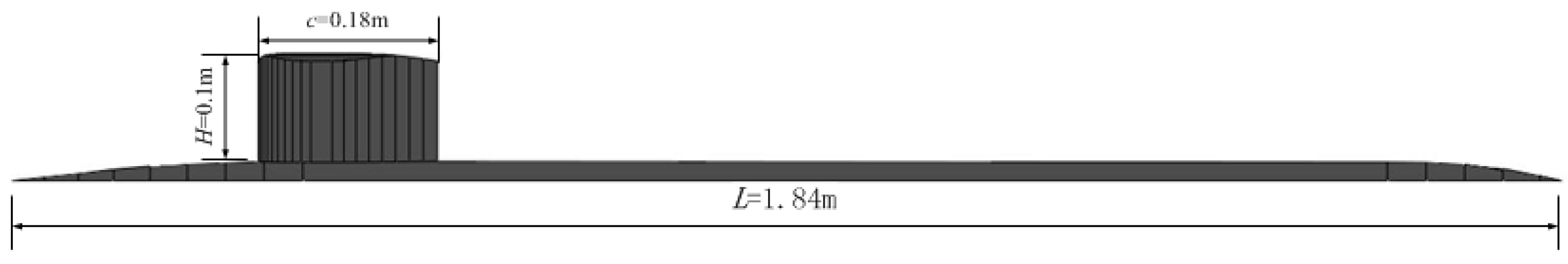
The model with a ratio of 1:48 and length of 184 cm is shown in Figure 2. The sail hull was also approximately considered to be the structure of an airfoil, of which the chord length was 18.4 cm.
3.2. The Parameters of Numerical Simulation
The finite volume method was used to solve the turbulence equations numerically, which was realized by the FLUENT codes. The outside of the model was the calculation domain of the flow field, with a rectangular shape. The distances between the model and inlet flow, the model and outlet flow, were 1 L and 2 L, respectively. The width of the flow field was 6c and the height was 3c, where c is the chord length. The boundary of computational domain, including the inlet, the outlet, the plane of the object, and the regions of the outside boundary, were set as the velocity inlet, the pressure outlet, the symmetrical boundary conditions, and the solid wall boundaries. The velocity of the flow was 8.68 m/s.
The method of wall function was combined with the RNG model to calculate the steady-state flow field, where, y+ ≈ 35, Re = 1.6 × 10⁷. The mesh thickness of the first boundary layer, namely, yp was 0.0001 m, which was obtained from Equation (21):
Considering time cost and computational power, we performed a steady-state grid-independent verification. We calculated the resistance value of the models with the grid number of 1 × 10⁶, 1.5 × 10⁶, 2 × 10⁶, 2.5 × 10⁶, 3 × 10⁶, 3.5 × 10⁶, and 4 × 10⁶. Through the comparison, we found that the grid number of 3 × 10⁶ could obtain the appropriate resistance. Therefore, the grid number of the flow field calculation was 3 × 10⁶. The transient simulation of the flow field was performed by the dynamic sub-lattice model in the LES.
We adopted a second order upwind scheme to discretize the convection term. We adopted the central difference scheme to discretize the diffusion term. Additionally, we adopted the second order implicit scheme to discretize the temporal term. We used the PISO method to solve the pressure–velocity coupling equation [37].
Since the maximum frequency of the analysis was 2 kHz, the time step was determined to be 2.5 × 10⁻⁴ s according to Equation (22). The number of samples was selected as 800 time steps to calculate the sound field.
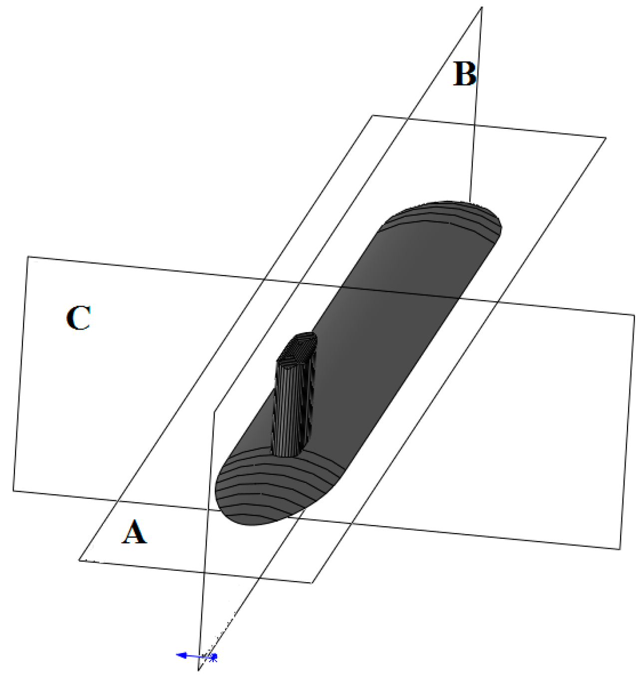
To analyze the flow field and the sound field in detail, some planes were set up as shown in Figure 3. Plane A is longitudinal and aligned with the center of the height of the sail hull. Plane B is longitudinal and aligned with the center of the thickness of the sail hull. Plane C is transversal and aligned with the center of the length of the sail hull.
4. The Flow Field of the Model
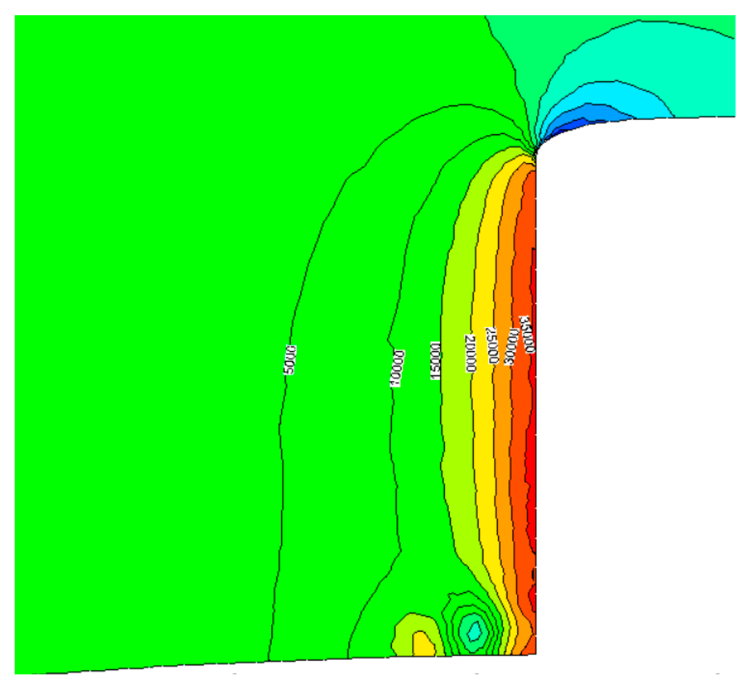
Figure 4 shows the leading edge’s pressure contour from Plane A and Plane B. Since the fluid is blocked by the leading edge, we observed that the pressure was becoming larger and larger when the points were close to the leading edge. Therefore, a large adverse pressure gradient existed at the sail hull’s leading edge.
The pressure gradient of the leading edge was adverse, compared to the flow stream. Then, the lateral vortices were generated by the influence of the adverse pressure gradient and arranged into eddies, which propagated in the downstream under the impact of the incoming flow and were hindered by the sail hull. Meanwhile, the leading edge of the sail hull was just like a bow, where the eddies ran along the sail hull and were deflected in the longitudinal direction to generate the longitudinal vortices. When the longitudinal vortices flow through the transition zone, the speed of the flow increases, so that the longitudinal vortices are stretched further. Finally, the horseshoe vortex was formed around the sail hull. The horseshoe vortex promotes the ability of flow separation between the submarine body and the sail hull, the flow separation also further enhances the intensity of the horseshoe vortex. Therefore, the horseshoe vortex with high intensity and weak dissipation was one of the flow-induced noise sources.
To show the three-dimensional structure of the horseshoe vortex in detail, the Q criterion was taken as the basis for the determination.
where is the tensor of the eddy, S is the tensor of strain rate.
The region with Q > 0 in the flow field could be considered as the core of the vortices, which revealed that the movement of the fluid was dominated by the rotation. Figure 5 shows the horseshoe vortex at Q = 500. The horseshoe vortex along the sail hull has a ‘U’ shape. The horseshoe vortex was formed at the leading edge, developed in the downstream, and dissipated slowly. The surface of the horseshoe vortex remained stable, and the legs of the horseshoe vortex were sturdy.
If the intensity of the horseshoe vortex can be effectively suppressed, the excitation force is weakened. Then, the flow-induced noise from the shell of the model excited by the horseshoe vortex is reduced. As we know, the mechanical VG is a device that changes the flow direction and brings the outside energy into the boundary layer. Hence, the separation of the boundary layer induced by the horseshoe vortex can be inhibited by the mechanical VG.
5. The Shape Selection of Mechanical VGs
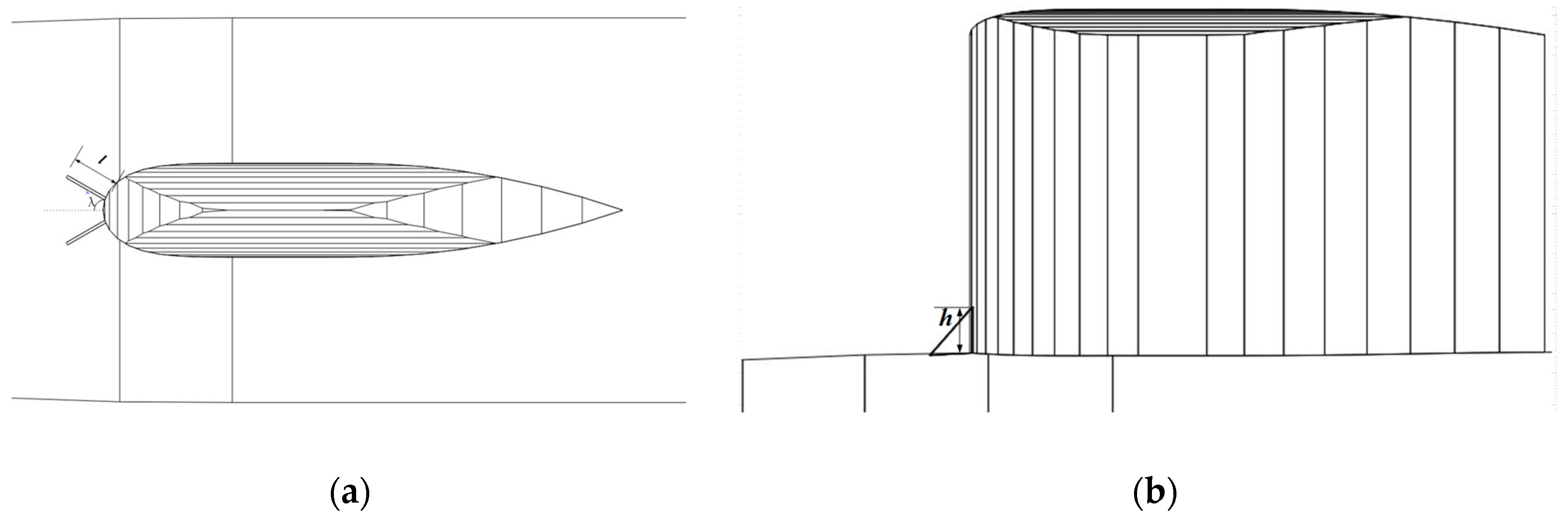
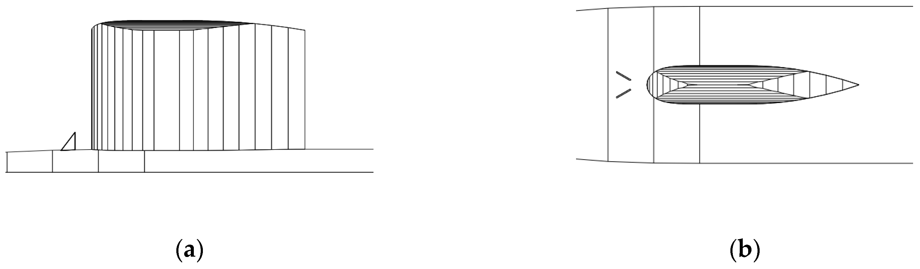
The VGs were symmetrically mounted on both sides of the model according to the central line, as shown in Figure 6. We used the λ to denote the angle of the mechanical VGs to the flow direction. The height of the mechanical VGs was 0.1 H, where, H was the height of the sail hull. The dimension of the mechanical VGs was higher than the thickness of the boundary layer on the surface of the submarine body. The length of the VGs was 0.1c, where c was the chord length of the sail hull.
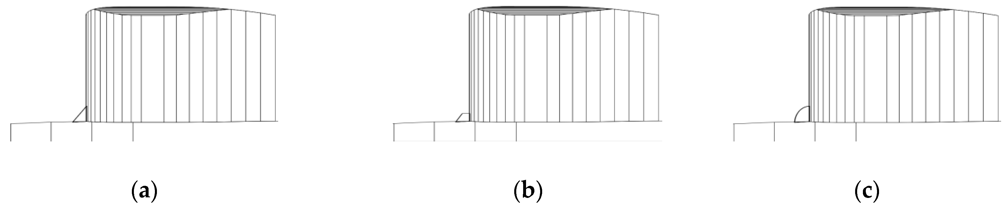
Considering the results of flow control in the air, we have investigated three shapes of mechanical VGs, semi-circular, triangular, and trapezoidal. The three shapes of mechanical VGs have the identical length of 0.1c, and the identical height of 0.1 H, where c is the chord length of the sail hull, and H is the height of sail hull. At the leading edge, we have placed a pair of different shapes of mechanical VGs with an angle of 30° to the flow direction. Figure 7 shows the placement of mechanical VGs of different shapes.
Figure 8 shows the comparison curves of radiated sound power from the original model and the models with semi-circular VGs, trapezoidal VGs, and triangular VGs. The models with trapezoidal VGs and triangular VGs had lower levels of radiated sound power than that of the original model. However, the radiated sound power from the model with semi-circular VGs was even higher than that of the original model. The corners of semi-circular VGs are not too sharp to produce enough vortices and cannot significantly destroy the formation of the horseshoe vortex. Therefore, the difference of the curves between the original model and the model with semi-circular VGs was minimal, especially in the low-frequency range. The addition of semi-circular VGs enhanced the level of radiated sound power in the high-frequency range, due to the VGs also vibrating.
We may conclude that semi-circular VGs cannot be utilized to suppress the flow-induced noise. Since the mechanical VGs with triangular and trapezoidal shapes have sharp corners and can produce enough vortices to change the horseshoe vortex’s formation, the radiated sound power from the models with these shapes is lower than that of the original model. There are two corners in trapezoidal VGs; the vortices of two adjacent groups are produced, while only one group of vortices are produced from triangular VGs. When the fluid flows around the two corners of the trapezoidal VGs, the vortices of the two adjacent groups rotate at a certain phase. Then, these vortices are weakened by each other. The control effect of the horseshoe vortex by trapezoidal VGs is less than that by triangular VGs. That is why triangular VGs have a better flow-induced noise suppression, compared to the other two shapes.
In Table 1, the total level of radiated sound power from the models with triangular and trapezoidal VGs is less than that of the original model in the frequency range from 10 Hz to 2000 Hz. The best noise reduction effect from mechanical VGs of the three shapes was the triangular. The conclusion is that if the flow-induced noise is suppressed by mechanical VGs, the VGs must have corners. If there is only one sharp corner in the VG, a better effect can be achieved.
6. The Optimized Angle of Mechanical VGs to the Flow Direction
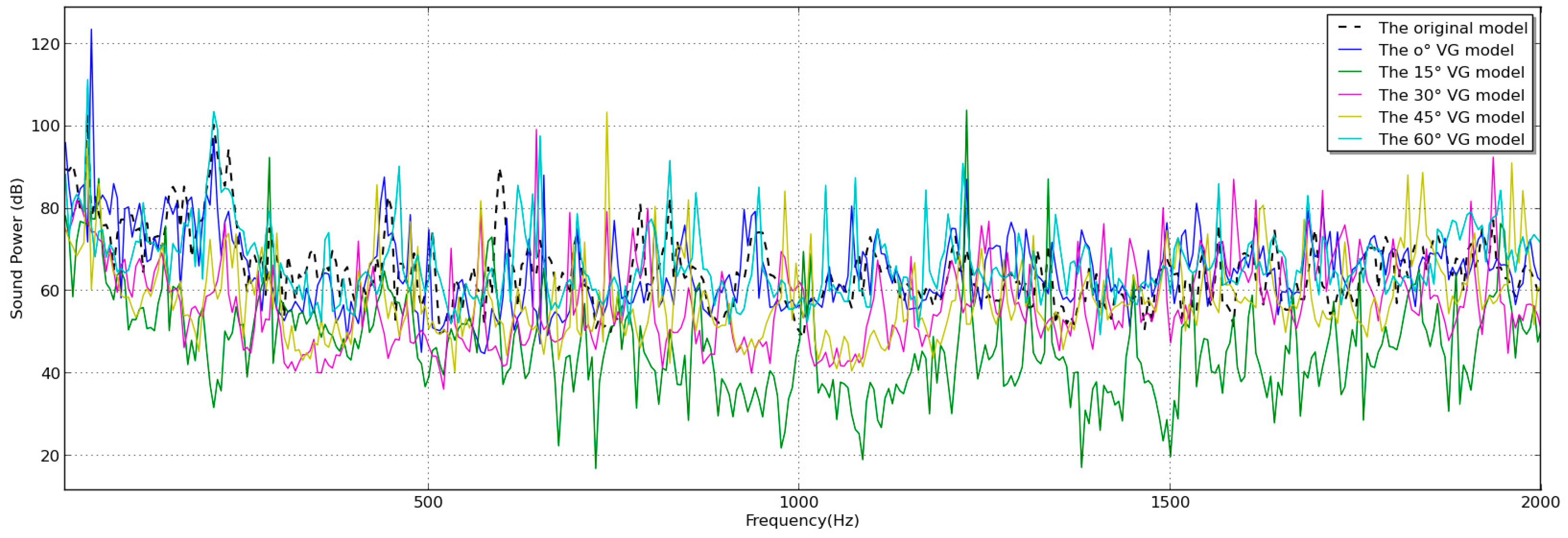
To reveal the optimum effect of the flow-induced noise suppression by mechanical VGs, we investigated the radiated sound power from the model with triangular VGs at different angles to the flow direction: 0°, 15°, 30°, 45°, and 60°. Figure 9 shows the curves of the radiated sound power from the original model and the model with triangular VGs at different angles to the flow direction.
The curve of the radiated sound power from the original model was similar to that from the model with triangular VGs. With the frequency increase, some peaks were observed. The level of the radiated sound power from the model with triangular VGs was higher than that of the original model in some frequencies. To better evaluate the noise reduction effect by the VGs, the total levels of radiated sound power from the original model and that with the triangular VGs are shown in Table 2.
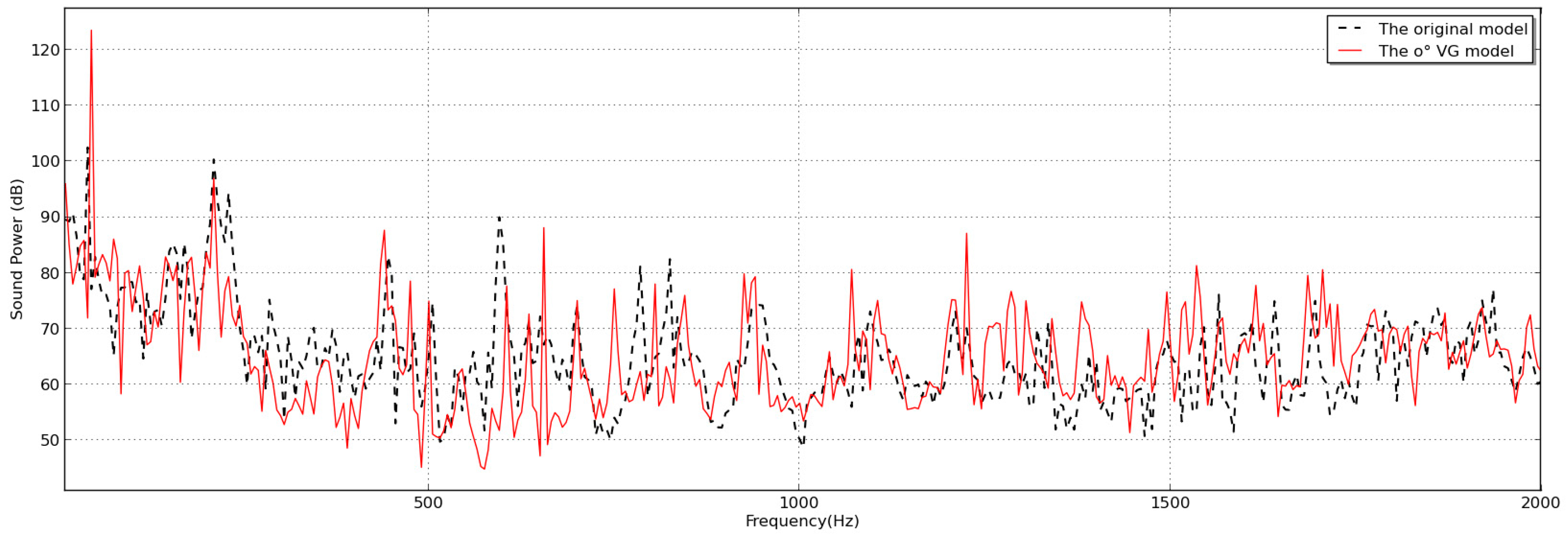
From Table 2, we see that with the increase in the angle, the total level of radiated sound power from the model with triangular VGs firstly decreased, and then increased. Therefore, to obtain a better noise reduction, there exists an optimum angle of VGs to the flow direction. The optimum angle is 30°, as shown in Table 2. When the angle of triangular VGs to the flow direction was 15°, 30°, and 45°, the flow-induced noise reduction could be 2.07 dB, 5.23 dB, and 1.48 dB, respectively. Meanwhile, at the angles of 0° and 60°, the noise reduction was negative. Therefore, the improper placement of triangular VGs increases the radiated sound power. The reason is that when the triangular VGs are placed at the angle of 0° to the flow direction, the VGs blockage strengthens the dimension of the lateral vortices, so that the intensity of the horseshoe vortex is enhanced. When the triangular VGs are placed at the angle of 45° or 60°, the VGs also strengthen the dimension of the lateral vortices and enhance the intensity of the horseshoe vortex. Figure 10 shows the curves of radiated sound power from the original model and the model with triangular VGs at the angle of 0° to the flow direction.
At the initial frequency range shown in Figure 10, the level of radiated sound power from the model with triangular VGs is 124 dB and is much larger than that of the original model, where the latter is 102 dB. A high peak at the frequency of 40 Hz was observed, which was caused by the horseshoe vortex excitation, not by the VGs. The dimension of VGs was too minimal compared to the wavelength of sound waves in the water; the efficiency of radiated sound power was too low. Therefore, the radiated sound power from the VGs themselves can be ignored. The triangular VGs had strengthened the lateral vortices, which were the origin of the horseshoe vortex. Then, the flow-induced noise from the shell excited by the horseshoe vortex was enhanced. In addition, the peak’s position in Figure 10 is not changed, even after the triangular VGs are placed. This phenomenon also shows that the high level at 40 Hz is not from the vibration of the VGs themselves. In the other frequency range, the radiated sound powers of the two models were similar to each other.
As we know, the evaluation of noise reduction is based on the total level of radiated sound power. Since the level difference of the two models at the initial frequency reached up to 22 dB, the total level of radiated sound power was mostly influenced by the difference, and the placement of the triangular VGs did not achieved the goal of noise reduction.
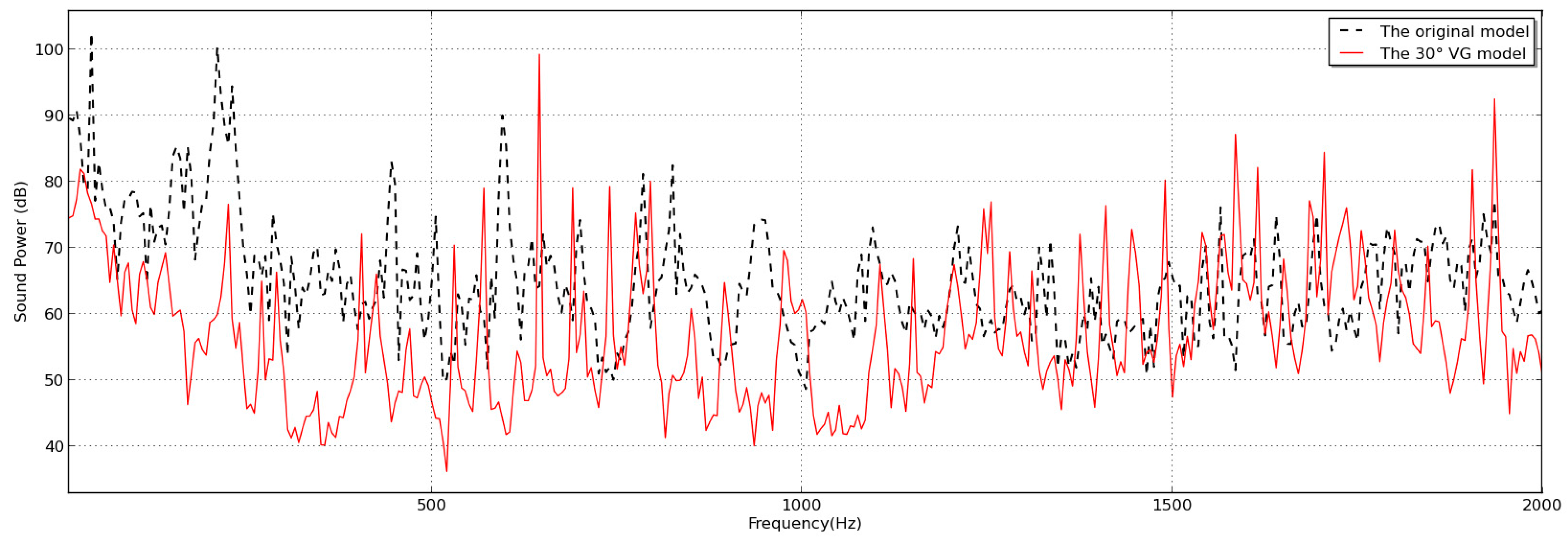
Figure 11 shows the level of radiated sound power from the original model and the model with triangular VGs at the angle of 30° to the direction of the flow. In the low-frequency range (f < 500Hz), the radiated sound power from the model with triangular VGs was lower than that from the original model. This phenomenon showed that the flow-induced noise was strongly weakened by the flow control of the triangular VGs. Therefore, the low-frequency hydrodynamic noise can be suppressed by the triangular VGs. The vortices generated by the mechanical VGs could change the structure of the horseshoe vortex. Specifically, the cluster of large-scale vortices could be changed into small-scale vortices.
At 650 Hz, a high peak was observed compared to the other frequencies. The frequency of the tail vortex shedding is
where St is the Strouhal number, U is the incoming flow velocity, and C is the feature length of the model. According to Equation (24), the frequency of the tail vortex shedding was 595 Hz, just as the black dotted line in Figure 11 indicates. This phenomenon indicated that the triangular VGs also changed the formation of the tail vortex shedding.
Figure 12 shows the turbulent kinetic energy contour at Plane A from the two models. In the wake flow field of the model with mechanical VGs, the area of intensive turbulence was somewhat larger than that of the original model. This phenomenon showed that the vortices produced by the mechanical VGs could influence the tail vortex shedding from the tail. The vortices could enhance the intensity of the wake. Meanwhile, these vortices were in the small-scale vortices. The flow-induced noise in the high-frequency range could be increased, because the flow-induced noise from the excitation of the small-scale vortices was mainly in the high-frequency range.
Since small-scale vortices from the triangular VGs can excite the shell of the model and generate the radiated sound power, more peaks were observed at the high-frequency range. Therefore, the utilization of the triangular VGs can shift the hydrodynamic noise from the low-frequency range to the high-frequency range through the flow control. As we know, the sound absorption in seawater is approximately proportional to the squared frequency. The low-frequency noise can propagate over a long distance and can be an efficient signal to detect underwater vehicles, while the high-frequency noise can be quickly absorbed by the seawater. Therefore, the triangular VGs provide a feasible method to suppress the low-frequency flow-induced noise.
7. The Mechanism of Noise Reduction by Triangular VGs
When the triangular VGs are set up at the leading edge of the sail hull, a new flow disturbance will occur in the fluids. We observed the change of adverse pressure gradient.
Figure 13 shows the pressure gradient of the leading edge at Plane B of the model with triangular VGs. Compared to Figure 4b, after the triangular VGs are placed, the change of the pressure gradient is not monotonous. Two eddies are at the bottom, which are the vortices from the corners of the triangular VGs. The pressure gradient of the eddies near the leading edge becomes small, which shows that the triangular VGs reduce the intensity of the adverse pressure gradient.
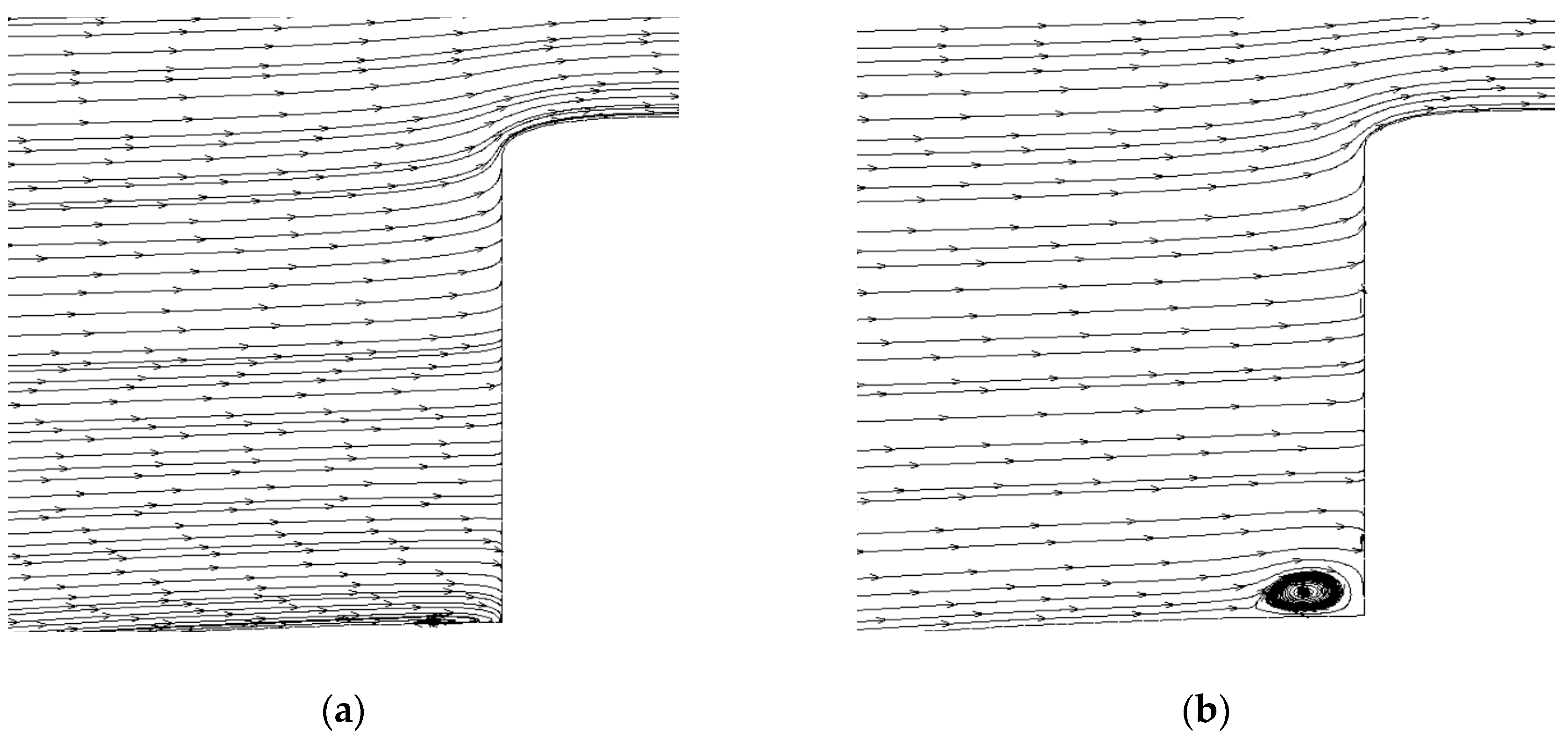
Figure 14 shows the streamline of the leading edge of the sail hull between the original model and the model with triangular VGs. When the triangular VGs were placed, a clockwise eddy was formed at the origin of the horseshoe vortex, as shown in Figure 14b. From the comparison, the vortex area was increased by 547% after the placement of the mechanical VGs. We can see that at the origin of the horseshoe vortex, the intensity of the eddies was significantly enhanced. That means the core area of the horseshoe vortex was expanded by the triangular VGs.
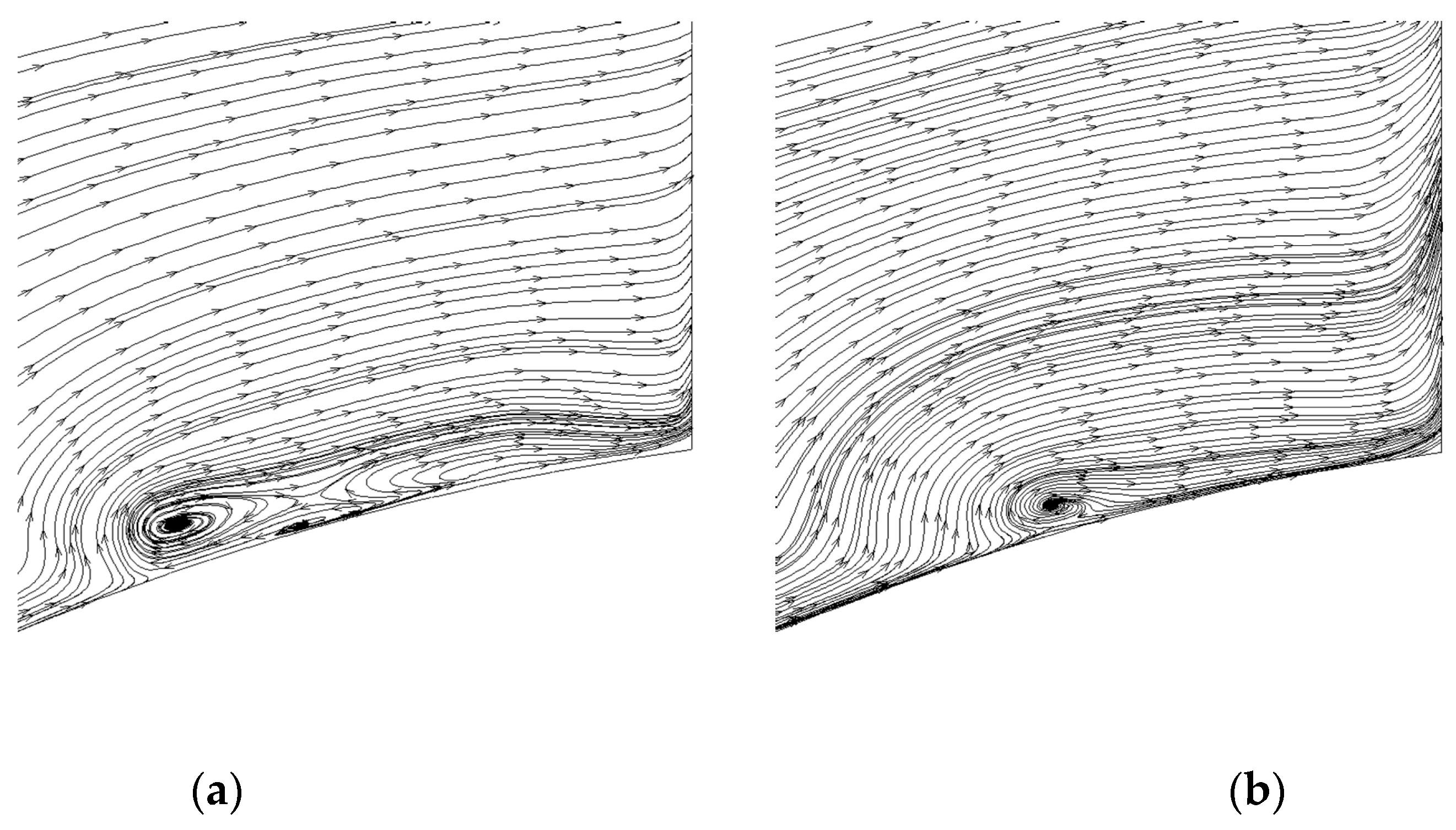
Figure 15 shows the streamline comparison between the original model and the model with triangular VGs at Plane C. A counter-clockwise eddy on the surface of the original model ran in a longitudinal direction. That is the origin of the horseshoe vortex, which moves continuously in the downstream, as shown in Figure 15a. After the triangular VGs were set up, the counter-clockwise eddy still ran in the longitudinal direction along the sail hull, but the core became small. The vortex area was decreased by 52% after the placement of the mechanical VGs. The streamlines continue to increase, as shown in Figure 15b. The core of the horseshoe vortex moved close to the surface, which revealed that the boundary layer separation was inhibited by the triangular VGs. Therefore, the intensity of the horseshoe vortex was weakened.
Figure 16 shows the diagram of the horseshoe vortex of the model with triangular VGs at Q = 500. Compared to Figure 5, the intensity of the horseshoe vortex at the origin becomes weak. The legs of the horseshoe vortex become shorter and are dissipated at the tail.
There exists a pressure difference between the two sides of the triangular VGs, which makes the fluid move from a high pressure to low pressure along the flow direction. Then, the spiral vortices are generated, which are opposite to the rotation of the horseshoe vortex. If the intensity of the horseshoe vortex at the origin decreases more than that in the downstream, the sail hull’s flow-induced noise will be reduced.
From the above analysis, the mechanism of the mechanical VGs to control the horseshoe vortex and reduce the flow-induced noise was obtained. We achieved the shape and the angle of the triangular VGs, but other parameters still need to be studied to obtain an optimum noise reduction.
8. The Optimized Distance between the VGs and the Sail Hull
Since the placement of triangular VGs is related to the generation of the lateral vortices, which can negatively influence the intensity at the origin and the running path of the horseshoe vortex, the distance from the triangular VGs to the leading edge of the sail hull must also have an optimized value. Similar to the VGs moving towards the mixture line in the air, we put the triangular VGs at distances of 0.1c, 0.15c, and 0.2c in front of the leading edge, where c is the chord length as shown in Figure 17. The flow field and the sound field in these cases were calculated.
The triangular VGs were at the angle of 30° to the direction of the flow. In the three cases, the pressure gradient change of the leading edge is shown in Figure 18.
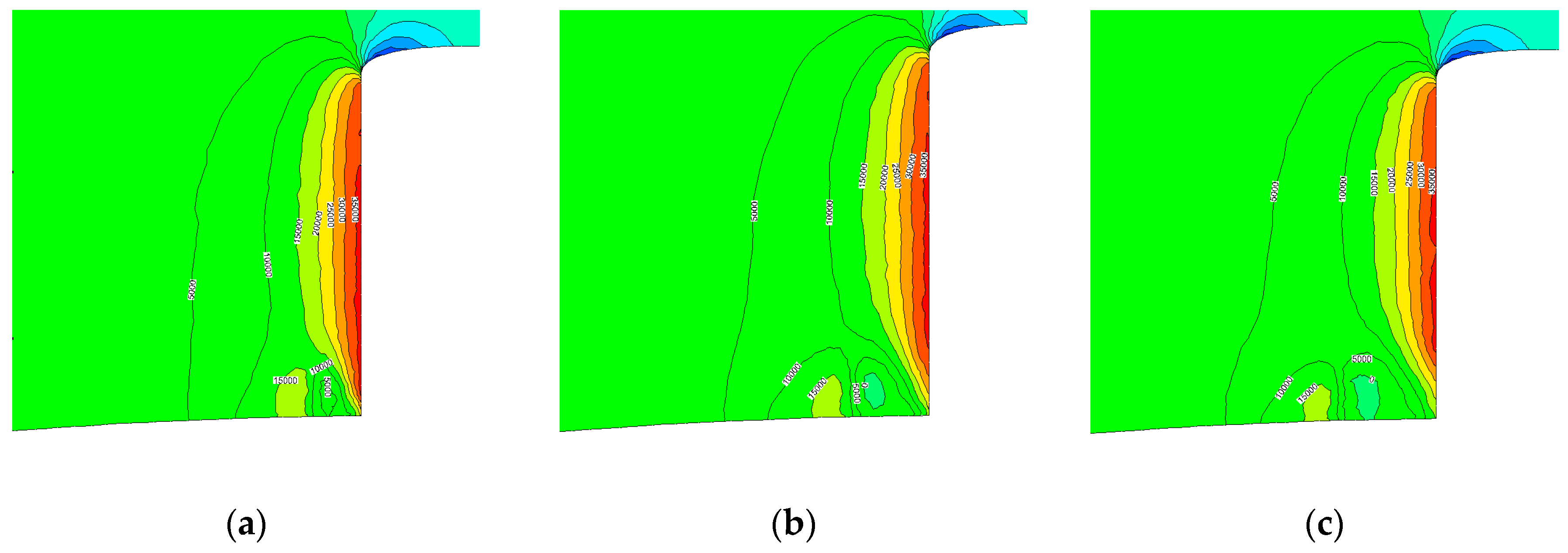
Compared to the original model, the triangular VGs stirred the turbulence. The pressure gradient stopped growing when the points were close to the leading edge. In other models, there exists turbulent disorders nearby the triangular VGs. The two new cores revealed the change in the pressure gradient, that is, one is adverse and the other is positive. The first core was the heads of triangular VGs, and the second core was the tails of triangular VGs.
Compared to Figure 11, the movement of the triangular VGs significantly changed the turbulence. We observed that the vortices from the VGs reduced the intensity of adverse pressure gradients at the leading edge of the sail hull. With the distance increase, the intensity changed and the turbulent disturbance became more obvious. The origin of the horseshoe vortex was intensively destroyed and the intensity of the horseshoe vortex was weakened. This phenomenon showed that the flow-induced noise by the excitation of the horseshoe vortex would be further reduced if the triangular VGs are moved far from the leading edge.
Figure 19 shows the streamline comparison between the original model and the model with triangular VGs at different distances from the leading edge. Compared to the original model, we observed that the origin of the horseshoe vortex was moved by the triangular VGs, and the dimension of the vortex core became small. The pressure gradient became mild, so that the formation intensity of the horseshoe vortex was decreased. In addition, the boundary layer separation was also delayed. Through the comparison, the vortex core changed by the triangular VGs was different, that is, the better effect was at 0.1c, where the vortex area had decreased by 53%, and the worse effect was at 0.15c, where the vortex area had increased by 94%. This phenomenon indicated that the position of the triangular VGs had an optimum value.
If the distance from the triangular VGs to the leading edge of the sail hull is too close, the formation of the horseshoe vortex is mostly influenced by the physical properties of the VGs. The flow velocity near the leading edge approaches zero, and no vortices can be generated from the corners. The function of the VGs is to shorten the connection between the leading edge and the submarine body. Therefore, in this situation, the shape of the mechanical VGs should be progressively ascending. However, if the distance from the mechanical VGs to the leading edge of the sail hull is beyond 0.2c, the vortices from the corners ascend with the flow and do not energize the boundary layer. The pressure gradient at the origin of the horseshoe vortex is minimally destroyed by the vortices. Therefore, the inhibition on the intensity of the horseshoe vortex is not apparent.
Figure 20 shows the streamline of Plane C between the original model and the model with triangular VGs at a distance of 0.1c from the leading edge of the sail hull. In the original model, two vortex cores were formed near the bottom of the model and the rotation direction of the cores were contrary. The position of each core was not identical in the mirror. Compared to the model with triangular VGs, the position of the two cores was closer to the surface, and the dimension of the two cores was smaller. This phenomenon showed that the boundary layer separation was inhibited by the triangular VGs. The streamline was smoother than the original model. The excitation energy from the turbulence fluctuation pressure was less than the original model. Therefore, radiated sound power from the model with triangular VGs was less than that of the original model.
Although the mechanical VGs are excited by the flow, the level of their radiated sound power is much less than the radiated sound power induced by the excitation of the horseshoe vortex in the original model. Since the dimension of the mechanical VGs was much less than the dimension of the model, the influence of the mechanical VGs on the flow-induced noise reduction from the excitation of the horseshoe vortex was the flow control.
Figure 21 shows the vortex quanta from the model with triangular VGs at a distance of 0.1c from the leading edge of the sail hull. Compared with Figure 4 and Figure 16, in the model with triangular VGs at a distance of 0.1c, the horseshoe vortex was split into two parts by the VGs. The two parts still surrounded the sail hull, that is, the head was in the leading edge, then the body, and the legs were dissipated in the tail. Compared to the original model, the body became slim and the legs became short. Then, the intensity of the horseshoe vortex was weakened. When the triangular VGs were placed near the leading edge of the sail hull, the left corner of the VG was adjacent to the surface and the right corner was far away from the surface. Even if the left corner was close to the surface, the vortices were generated and developed at a short distance. The vortices from the right corner were not obvious, due to the influence of the horseshoe vortex. Since the dimension of the mechanical VGs was too small and the increased control of the flow was obvious, it was a good thing that achieved much while requiring limited change to the system.
In Figure 22, after the triangular VGs are placed on the model, the peaks in the frequency range less than 500 Hz disappeared. This showed that the triangular VGs reduced the intensity of the horseshoe vortex. However, the peak at 595 Hz shifts, but does not disappear. This showed that the suppression of the horseshoe vortex by the triangular VGs could influence the vortices shedding from the tail of the sail hull.
In Table 3, the level of noise reduction by the triangular VGs is mostly above 6 dB. This shows that the flow-induced noise from the model has been reduced by up to 50% in the distance of sound propagation. Therefore, it is possible to believe that the acoustic stealth performance of submarines would be enhanced if the mechanical VGs were set up.
The noise reduction comparison of the triangular VGs at different distances with the original model showed that the placement of the VGs was according to the following rule: the higher corner must be in the origin of the horseshoe vortex. The vortices from the higher corner can inhibit the formation of the horseshoe vortex. The VGs can also inject the outside energy into the boundary layer and reduce the change in the pressure gradient. Then, the separation of the boundary layer is inhibited. Since the origin of the horseshoe vortex was formed at a distance of 0.1c from the leading edge of the sail hull, the triangular VGs at this distance achieved the optimum suppression of the flow-induced noise.
Through numerical calculations, the resistance of the model was changed from 35.698 N to 38.299 N, when the triangular VGs were installed on the model with the optimum hydrodynamic noise reduction effect. The resistance was increased by 7.29%.
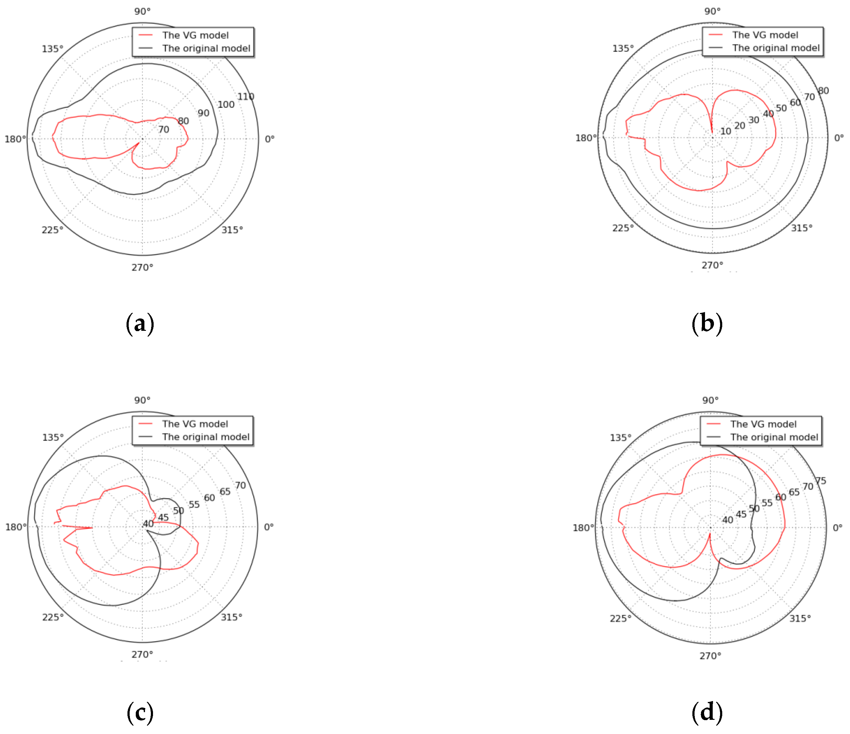
Figure 23 shows the horizontal directivity of the sound field from the two models. In the low-frequency range, the horizontal directivity of the sound field from the model with the triangular VGs was less intensive than that of the original model. This phenomenon showed that the horseshoe vortex had been successfully been suppressed. However, the sound pressure in the leading edge and the trailing edge was still intensive. In the high-frequency range, the directivity of the sound field of the model with the triangular VGs became milder than that of the original model, even if the wake flow field had been affected by the mechanical VGs.
9. The Experimental Validation
To evaluate the flow-induced noise reduction effect by the mechanical VGs and to validate the analysis of the numerical simulations, the hydrodynamic noise from the original model and the model with the mechanical VGs were measured in a gravity water tunnel at the Harbin Engineering University.
9.1. The Theory of Reverberation Method
If a complex underwater noise source is setup in a free environment, the mean square sound pressure at a distance, r, from the source is
where W0 is the radiated sound power, Pe is the effective sound pressure, is the density, and c0 is the velocity of the sound waves.
If the same noise source is placed in the reverberation tank, the mean square sound pressure is,
where is a constant of the reverberation water tank, and is the sound attenuation coefficient. Since the coefficient of sound attenuation in the water medium is smaller than the coefficient in the boundaries of the reverberation tank, the coefficient of sound attenuation in the water medium can be ignored.
The radiated sound power of the noise source in the far-field can be expressed as,
Through the comparison of Equations (26) and (27),
Then,
where is the level of sound pressure of the noise source, is the level of spatial average sound pressure in the reverberation area, is a correction factor, which represents the difference of the sound pressure level between the reverberation field and the free field. The level difference can also be expressed as
where , T60 is the reverberation time, and V is the whole reverberation tank’s volume.
9.2. The Description of the Experimental Measurement
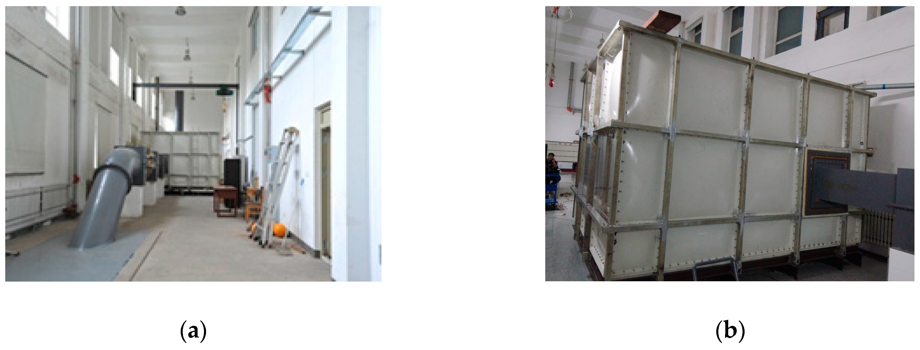
The gravity water tunnel was composed of a water tank, a contraction section, a rectifying section, a working section, a diffusion section, and the pipes. The models were installed in the working section. To reduce the vibration from the other sections, an iron sand box and a Helmholtz muffler were installed at both ends of the working section. Outside the working section, a reverberation tank made up of steel and plastic is shown in Figure 24. The bottom of the reverberation tank was vibration-damped to eliminate ground vibration.
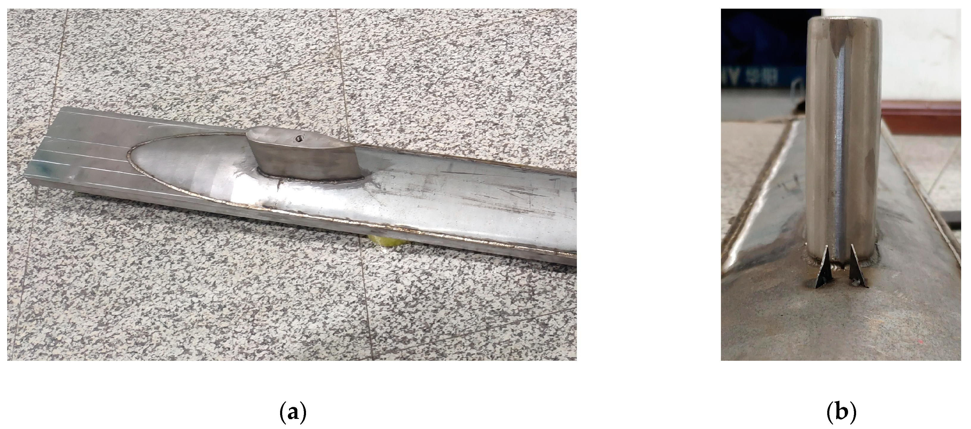
Figure 25 shows the picture of the original model and the model with mechanical VGs. The parameters were as follows: the mechanical VGs were triangular; the mechanical VGs were at an angle of 30° to the flow direction; the mechanical VGs were 0.1 H high and 0.1c long, where H was the height of the sail hull and c was the chord length; the mechanical VGs were setup at a distance of 0.1c from the leading edge of the sail hull.
The radiated sound power from the two models was recorded by the reverberation method. Owing to the measured limitation frequency of the reverberation tank, we put a fluctuation pressure sensor on the top surface of the sail hull to measure the turbulent fluctuation pressure instead of the inside placement of a hydrophone, because the hydrophone’s sensitivity was lower than the sensor’s sensitivity.
Figure 26 shows a vertical array of five hydrophones in the reverberation area to measure the spatial average sound pressure in the reverberation tank. The radiated sound power of the hydrodynamic noise was obtained according to Equation (29).
The measured limitation frequency using the reverberation method in the reverberation tank was estimated as 500 Hz. Below this frequency, we could compare the sensitivities from the fluctuation pressure sensor and the hydrophone to estimate the sound pressure level from the data of the fluctuation pressure sensor. Therefore, we could achieve the total level of radiated sound power. The velocity of water flow was 4.62 m/s and 8.68 m/s. Figure 27 shows the turbulent fluctuation pressure collected by the fluctuation pressure sensor.
In Figure 27, we observed that the turbulent fluctuation pressure was suppressed in the low-frequency range by the triangular VGs. However, a high peak was observed at a frequency of 50 Hz. Through a detailed analysis, we found that the pressure level at this frequency remained unchanged in the two experimental measurements. First, in the measurement of the original model, and second, the measurement of the model with the mechanical VGs. Then, we could conclude that this peak was generated by the electricity power supply. Since the fluctuation pressure sensor must be amplified by a conditioner, the conditioner could only work under the alternate current (AC) supply. In our country, the frequency of the AC supply is 50 Hz. Therefore, the high peak of 50 Hz came from the AC supply, and not from the flow-induced noise. In the analysis, we neglected this peak.
Compared with Figure 11, we observe that the trend of the pressure changing with the frequency is very similar. If the frequency was less than 1200 Hz, the mechanical VGs could suppress the hydrodynamic noise. Meanwhile, if the frequency was higher than 1200 Hz, the mechanical VGs could enhance the hydrodynamic noise. Influenced by the background noise, the peaks in Figure 27 are greater than the peaks in Figure 11.
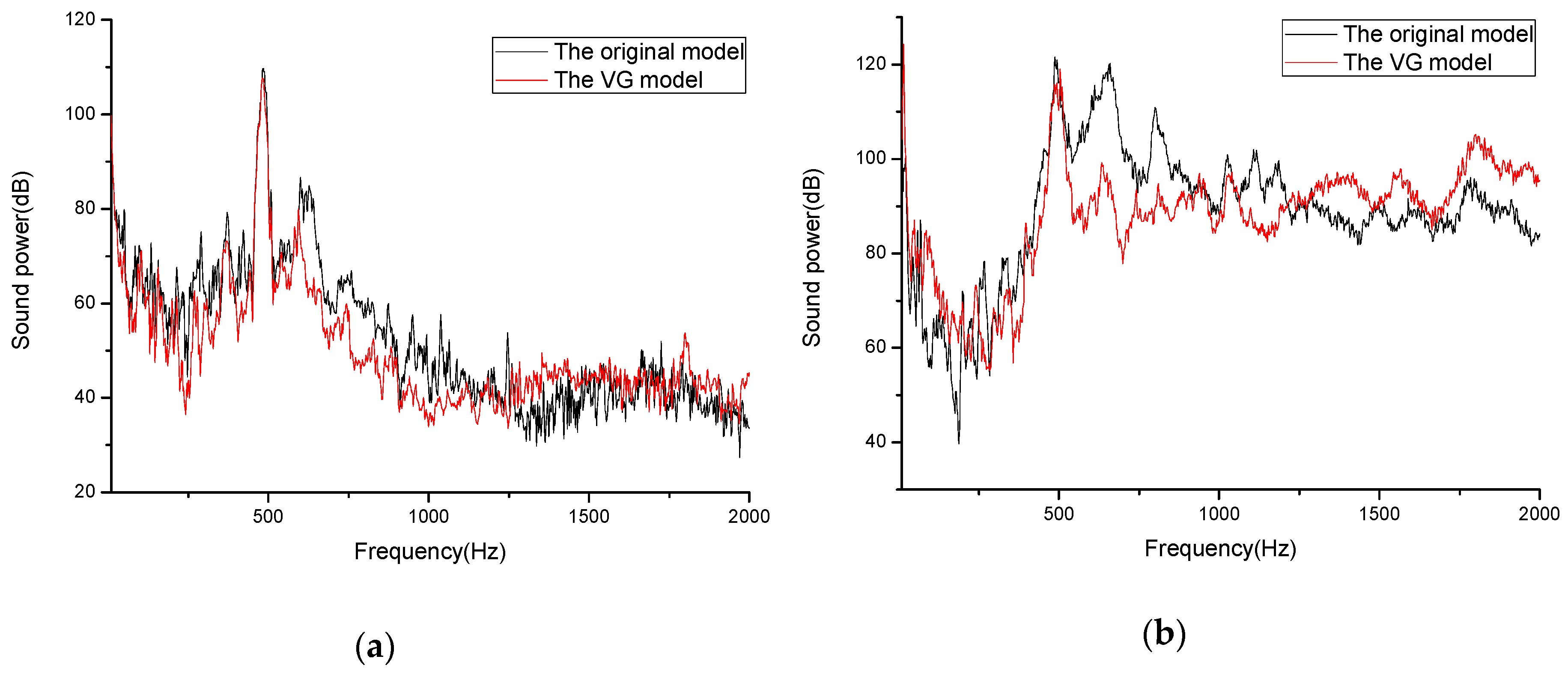
Figure 28 shows the radiated sound power collected in the reverberation tank. We observed that when the frequency was less than 500 Hz, the radiated sound power from the two models was especially low. This phenomenon clearly showed the measured limitation frequency, which was an intrinsic property of the reverberation tank.
In Figure 28a, we can see that the fluctuation pressure in the low-frequency range was reduced by the triangular VGs. The radiated sound power was also decreased by the mechanical VGs. The radiated sound power was obviously reduced when f < 1200 Hz. Since the signal-to-noise ratio was too low, the radiated sound powers of the two models were very similar to each other when f > 1200 Hz. The radiated sound power from the model with the triangular VGs was even larger than that from the original model, due to the interference of the background noise. At a flow velocity of 4.62 m/s, the total radiated power reduction level by the mechanical VGs was 3.67 dB. Owing to the time limitation, we did not calculate the flow-induced noise from the models at the flow velocity of 4.62 m/s.
In Figure 28b, if the frequency is less than 1200 Hz, the radiated sound power from the model with the mechanical VGs is less than the original model. Meanwhile, if the frequency was higher than 1200 Hz, the radiated sound power from the model with the mechanical VGs is larger than the original model. The trend of radiated sound power changing with the frequency in Figure 28b was the same as that in Figure 11.
Through the statistical analysis, we found that the total radiated sound power of the two models was approximately proportional to the sixth power of the flow velocity. This phenomenon agreed well with the law of hydrodynamic noise. Through the comparison of the two models, the noise reduction of the radiated sound power by the mechanical VGs was 7.93 dB at a flow velocity of 8.68 m/s. However, the calculated noise reduction of the radiated sound power was 8.93 dB at a flow velocity of 8.68 m/s, as shown in Table 3. The reasons for the differences between the numerical simulation and the experiment measurement were as follows:
First, the sail hull was welded on a part of the submarine body. The experimental model was not as smooth as that in the numerical simulation. The welded points can affect the formation of the horseshoe vortex.
Second, the thickness of the models in the numerical simulation was identical. However, the thickness of the models in the experiment was not identical, due to issues relating to mechanical manufacture.
Third, no background noise exists in the numerical simulation. In the experiment, we could not avoid background noise from the ground, the circular pipes, the power supply, etc., even if we did our best to reduce these background noise effects.
Fourth, there were also some other interferences. For example, the water temperature, the flow velocity repetition, and the boundary conditions in the experiment were not considered to be rigid.
However, the measured hydrodynamic noise suppression level was only 1dB lower than the calculated noise suppression level. The models in the simulation and experiment were much smaller compared to real submarines, but the noise reduction effect was obvious. We may conclude that if the mechanical VGs are placed on a larger model, the noise reduction could be more considerable. Therefore, we believe that the proposed noise reduction method by the mechanical VGs in our research can be applied to enhance the acoustic stealth performance of underwater vehicles in the future.
10. Conclusions
In the aviation field, mechanical VGs were successfully applied to control the flow separation. However, the noise reduction from the flow control by the VGs has not been fully considered, especially in water. We proposed a method whereby mechanical VGs were used to inhibit the formation of the horseshoe vortex and reduce the force from the horseshoe vortex. Then, the flow-induced noise can be suppressed. In our study, we created the model according to the structure of the SUBOFF. The flow field was calculated by a combination between the large eddy simulation and the RNG k-Ɛ turbulent model. The flow-induced noise was estimated by the wavenumber–frequency spectrum. The flow-induced noise was calculated using Lighthill’s acoustic analogy and the finite element method. Through the comparison, we investigated the change in the flow field and the sound field, when the mechanical VGs were placed at the leading edge of the sail hull. Through the investigation of the shapes of the VGs, the angles of the VGs to the direction of the flow, and the distances of the VGs to the leading edge of the sail hull, we summarized the optimum parameters of the VGs, based on comparisons with the original model. After that, we created a steel model according to the simulation. The experiment was carried out in a gravity water tunnel, based on the reverberation method. The simulation results were validated by the experiment. The conclusions of this research are as follows:
First, the triangular VGs have a better effect in noise reduction. We found that the high corner of the triangular VGs will produce the vortices, which are opposite to the rotation of the horseshoe vortex. The vortices from the low corner can inject the outside energy into the boundary layer and reduce the pressure gradient. All these vortices can decrease the intensity of the horseshoe vortex.
Second, the angle of the triangular VGs has an important influence on the noise reduction. Better noise reduction is achieved when the angle of the triangular VGs to the direction of the flow is 30°.
Third, the distance from the triangular VGs to the leading edge of the sail hull is related to the effect of the noise reduction. Better noise reduction can be achieved when the triangular VGs are placed at a distance of 0.1c, and the high corner of the VGs is placed at the origin of the horseshoe vortex, where c is the chord length.
Fourth, we found that when the triangular VGs, with a length of 0.1c and the height of 0.1 H, are placed at a distance of 0.1c and at an angle of 30° to the flow direction, the optimum reduction of the flow-induced noise is 8.93 dB, where H is the sail hull’s height.
Fifth, the noise reduction level of the flow-induced noise in the experimental measurement was in good accordance with that in the simulation. Therefore, the analysis of the numerical calculation was validated.
The proposed method of flow-induced noise reduction by the mechanical VGs can be applied to reduce the hydrodynamic noise from underwater vehicles, such as the submarines, torpedoes, the UUV, etc.
Author Contributions
Writing—original draft preparation, Y.L. (Yalin Li); writing—review and editing, Y.L. (Yongwei Liu); visualization, H.J.; supervision, D.S.
Funding
This research was funded by the steady support plan from the Acoustic Science and Technology Laboratory, grant number SSJSWDZC2018005, the project from Key Laboratory of Acoustic Stealth, grant number 614220405011706, and the project from Acoustic Science and Technology Laboratory, grant number 6142108011305.
Acknowledgments
The authors would like to thank Peichun Amy Tsai of the University of Alberta.
Conflicts of Interest
The authors declare no conflict of interest.
References
- Yu, M.; Wu, Y.; Pang, Y. A review of progress for hydrodynamic noise of ships. J. Ship Mech. 2007, 11, 152–158. [Google Scholar]
- Li, D.Q.; Hallander, J.; Johansson, T. Predicting underwater radiated noise of a full scale ship with model testing and numerical methods. Ocean Eng. 2018, 161, 121–135. [Google Scholar] [CrossRef]
- Fouatih, O.M.; Medale, M.; Imine, O.; Imine, B. Design optimization of the aerodynamic passive flow control on NACA 4415 airfoil using vortex generators. Eur. J. Mech. B/Fluids 2016, 56, 82–96. [Google Scholar] [CrossRef]
- Tao, S.; Tang, A.; Xin, D.; Liu, K.; Zhang, H. Vortex-induced vibration suppression of a circular cylinder with vortex generators. Shock Vib. 2016, 1–10. [Google Scholar] [CrossRef]
- Kuya, Y.; Takeda, K.; Zhang, X. Computational investigation of a race car wing with vortex generators in ground effect. J. Fluids Eng. 2010, 132, 1–8. [Google Scholar] [CrossRef]
- Lin, J.C. Review of research on low-profile vortex generators to control boundary-layer separation. Prog. Aerosp. Sci. 2002, 38, 389–420. [Google Scholar] [CrossRef]
- Brüderlin, M.; Zimmer, M.; Hosters, N.; Behr, M. Numerical simulation of vortex generators on a winglet control surface. Aerosp. Sci. Technol. 2017, 71, 651–660. [Google Scholar] [CrossRef]
- Titchener, N.; Babinsky, H. A review of the use of vortex generators for mitigating shock-induced separation. Shock Waves 2015, 25, 473–494. [Google Scholar] [CrossRef]
- Rybalko, M. Aerodynamic impact of vortex generators on a relaxed-compression low-boom inlet. AIAA J. 2015, 53, 3700–3711. [Google Scholar] [CrossRef]
- Boniface, J.-C. A computational framework for helicopter fuselage drag reduction using vortex generators. J. Am. Helicopter Soc. 2016, 61, 1–13. [Google Scholar] [CrossRef]
- Hoffmann, F.; Schmidt, Ha.; Nayeri, C.; Paschereit, O. Drag reduction using base flaps combined with vortex generators and fluidic oscillators on a bluff body. Int. J. Commer. Veh. 2015, 8, 705–712. [Google Scholar] [CrossRef]
- Gao, L.; Zhang, H.; Liu, Y.; Han, S. Effects of vortex generators on a blunt trailing-edge airfoil for wind turbines. Renew. Energy 2015, 76, 303–311. [Google Scholar] [CrossRef]
- Verma, S.B.; Manisankar, C.; Raju, C. Control of shock unsteadiness in shock boundary-layer interaction on a compression corner using mechanical vortex generators. Shock Waves 2012, 22, 327–339. [Google Scholar] [CrossRef]
- Lee, S.; Loth, E. Supersonic boundary-layer interactions with various micro-vortex generator geometries. Aeronaut. J. 2009, 113, 683–697. [Google Scholar] [CrossRef]
- Verma, S.B.; Chidambaranathan, M. Transition control of Mach to regular reflection induced interaction using an array of micro ramp vane-type vortex generators. Phys. Fluids 2015, 27, 1–23. [Google Scholar] [CrossRef]
- Godard, G.; Stanislas, M. Control of a decelerating boundary layer. Part 1: Optimization of passive vortex generators. Aerosp. Sci. Technol. 2006, 10, 181–191. [Google Scholar] [CrossRef]
- Lo, K.H.; Kontis, K. Flow characteristics over a tractor-trailer model with and without vane-type vortex generator installed. J. Wind Eng. Ind. Aerodyn. 2016, 159, 110–122. [Google Scholar] [CrossRef]
- Zhang, Y.; Hu, S.; Zhang, Xu.; Benner, M.; Mahallati, A.; Vlasic, E. Flow control in an aggressive interturbine transition duct using low profile vortex generators. J. Eng. Gas Turbines Power 2014, 136, 1–8. [Google Scholar] [CrossRef]
- Lengani, D.; Simoni, D.; Ubaldi, M.; Zunino, P.; Bertini, F. Turbulent boundary layer separation control and loss evaluation of low profile vortex generators. Exp. Therm. Fluid Sci. 2011, 35, 1505–1513. [Google Scholar] [CrossRef]
- Törnblom, O.; Johansson, A.V. A Reynolds stress closure description of separation control with vortex generators in a plane asymmetric diffuser. Phys. Fluids 2007, 19, 1–15. [Google Scholar]
- De Tavernier, D.; Baldacchino, D.; Ferreira, C. An integral boundary layer engineering model for vortex generators implemented in XFOIL. Wind Energy 2018, 21, 906–921. [Google Scholar] [CrossRef]
- Li, Q.; Liu, C. Declining angle effects of the trailing edge of a microramp vortex generator. J. Aircr. 2010, 47, 2086–2095. [Google Scholar] [CrossRef]
- Wang, H.; Zhang, B.; Qiu, Q.; Xu, X. Flow control on the NREL S809 wind turbine airfoil using vortex generators. Energy 2017, 118, 1210–1221. [Google Scholar] [CrossRef]
- Jirasek, A. Vortex generator model and its application to flow control. J. Aircr. 2005, 42, 1486–1491. [Google Scholar] [CrossRef]
- Joubert, G.; le Pape, A.; Heine, B.; Huberson, S. Vortical interactions behind deployable vortex generator for airfoil static stall control. AIAA J. 2013, 51, 240–252. [Google Scholar] [CrossRef]
- Yan, Y.; Chen, L.; Li, Q.; Liu, C. Numerical study of micro-ramp vortex generator for supersonic ramp flow control at Mach 2.5. Shock Waves 2017, 27, 79–96. [Google Scholar] [CrossRef]
- Bao, D.; Jia, Q.; Zhang, Z. Effect of vortex generator on flow field quality in 3/4 open jet automotive wind tunnel. SAE Int. J. Passeng. Cars Mech. Syst. 2017, 10, 224–234. [Google Scholar] [CrossRef]
- Von stillfried, F.; Wallin, S.; Johansson, A.V. Evaluation of a vortex generator model in adverse pressure gradient boundary layers. AIAA J. 2011, 49, 982–993. [Google Scholar] [CrossRef]
- Giepman, R.H.M.; Schrijer, F.F.J.; van Oudheusden, B.W. Flow control of an oblique shock wave reflection with micro-ramp vortex generators, effects of location and size. Phys. Fluids 2014, 26, 1–16. [Google Scholar] [CrossRef]
- Zhang, B.; Zhao, Q.; Xiang, X.; Xu, J. An improved micro-vortex generator in supersonic flows. Aerosp. Sci. Technol. 2015, 47, 210–215. [Google Scholar] [CrossRef]
- Suarez, J.M.; Flaszynski, P.; Doerffer, P. Application of rod vortex generators for flow separation reduction on wind turbine rotor. Wind Energy 2018, 21, 1202–1215. [Google Scholar] [CrossRef]
- Součková, N.; Kuklová, J.; Popelka, L.; Matějka, M. Visualization of flow separation and control by vortex generators on an single flap in landing configuration. EPJ Web Conf. 2012, 25, 1–12. [Google Scholar]
- Martinez-filgueira, P.; Fernandez-Gamiz, U.; Zulueta, E.; Errasti, I.; Fernandez-Gauna, B. Parametric study of low-profile vortex generators. Int. J. Hydrogen Energy 2017, 42, 17700–17712. [Google Scholar] [CrossRef]
- Kaltenbacher, M.; Escobar, M.; Becker, S.; Ali, I. Numerical simulation of flow-induced noise using LES/SAS and Lighthill’s acoustic analogy. Int. J. Numer. Methods Fluids 2010, 63, 1103–1122. [Google Scholar] [CrossRef]
- Germano, M.; Piomelli, U.; Moin, P. A dynamic subgrid-scale eddy viscosity model. Phys. Fluids 1991, 3, 1760–1765. [Google Scholar] [CrossRef]
- Heatwole, C.M.; Franchek, M.A.; Bernhard, R.J. A robust feedback controller implementation for flow induced structural radiation of sound. In Proceedings of the INTER-NOISE and NOISE-CON Congress and Conference, Seattle WA, USA, 29 September 1996; Institute of Noise Control Engineering: Reston, VA, USA, 1996. [Google Scholar]
- Zhang, N.; Xie, H.; Wang, X.; Wu, B. Computation of votical flow and flow induced noise by large eddy simulation with FW-H acoustic analogy and Powell vortex sound theory. J. Hydrodyn. 2016, 28, 255–266. [Google Scholar] [CrossRef]
Figure 1.
The comparison curve between the numerical simulation and the experimental test. The dark line denotes the preliminary test, and the red line denotes the numerical calculation. The frequency is in the range from 0 to 1000 Hz. The reference sound pressure level is 20 uPa.
Figure 1.
The comparison curve between the numerical simulation and the experimental test. The dark line denotes the preliminary test, and the red line denotes the numerical calculation. The frequency is in the range from 0 to 1000 Hz. The reference sound pressure level is 20 uPa.

Figure 2.
The diagram of the model. The model is a whole sail hull with part of the body. The dimension is scaled from the SUBOFF model. The length (L) of the sail hull is 184 cm. The height (H) of the sail hull is 10 cm. The chord length (c) is 18.4 cm.
Figure 2.
The diagram of the model. The model is a whole sail hull with part of the body. The dimension is scaled from the SUBOFF model. The length (L) of the sail hull is 184 cm. The height (H) of the sail hull is 10 cm. The chord length (c) is 18.4 cm.

Figure 3.
The diagram of the planes. Plane A is in the longitudinal direction, Plane B is in the longitudinal direction, and Plane C is in the transversal direction.
Figure 3.
The diagram of the planes. Plane A is in the longitudinal direction, Plane B is in the longitudinal direction, and Plane C is in the transversal direction.

Figure 4.
The pressure contour at the leading edge of Plane A and Plane B. The pressure is from 5000 Pa to 35,000 Pa, when the points are approaching to the leading edge. (a) Plane A; (b) Plane B.
Figure 4.
The pressure contour at the leading edge of Plane A and Plane B. The pressure is from 5000 Pa to 35,000 Pa, when the points are approaching to the leading edge. (a) Plane A; (b) Plane B.

Figure 5.
The diagram of the horseshoe vortex nearby the sail hull.

Figure 6.
The sketch of the mechanical VGs on the model. (a) Top view; (b) side view.

Figure 7.
The mechanical vortex generators (VGs) on the model: (a) triangular; (b) trapezoidal; (c) semi-circular.
Figure 7.
The mechanical vortex generators (VGs) on the model: (a) triangular; (b) trapezoidal; (c) semi-circular.

Figure 8.
The radiated sound power from the original model and the models with three shapes of mechanical VGs.
Figure 8.
The radiated sound power from the original model and the models with three shapes of mechanical VGs.

Figure 9.
The comparison curve of radiated sound power from the original model and the model with triangular VGs at different angles to the flow direction. ‘The 0° VG’ means that the triangular VGs are at the angle of 0° to the flow direction. The other meanings are the same as ‘The 0° VG’.
Figure 9.
The comparison curve of radiated sound power from the original model and the model with triangular VGs at different angles to the flow direction. ‘The 0° VG’ means that the triangular VGs are at the angle of 0° to the flow direction. The other meanings are the same as ‘The 0° VG’.

Figure 10.
The comparison curve of radiated sound power between the original model and the model with triangular VGs at the angle of 0° to the flow direction.
Figure 10.
The comparison curve of radiated sound power between the original model and the model with triangular VGs at the angle of 0° to the flow direction.

Figure 11.
The curve of radiated sound power from the original model and the model with triangular VGs at the angle of 30° to the flow direction.
Figure 11.
The curve of radiated sound power from the original model and the model with triangular VGs at the angle of 30° to the flow direction.

Figure 12.
The wake flow field of the two models. (a) The original model; (b) the model with the mechanical VGs.
Figure 12.
The wake flow field of the two models. (a) The original model; (b) the model with the mechanical VGs.

Figure 13.
The pressure gradient of the leading edge at Plane B of the model with triangular VGs. Two eddies from the triangular VGs can be clearly observed.
Figure 13.
The pressure gradient of the leading edge at Plane B of the model with triangular VGs. Two eddies from the triangular VGs can be clearly observed.

Figure 14.
The streamline near the leading edge of Plane B between the original model and the model with triangular VGs. (a) The original model; (b) the model with triangular VGs.
Figure 14.
The streamline near the leading edge of Plane B between the original model and the model with triangular VGs. (a) The original model; (b) the model with triangular VGs.

Figure 15.
The local streamline of Plane C between the original model and the model with triangular VGs. (a) The original model; (b) the model with triangular VGs.
Figure 15.
The local streamline of Plane C between the original model and the model with triangular VGs. (a) The original model; (b) the model with triangular VGs.

Figure 16.
The diagram of the horseshoe vortex of the model with triangular VGs.

Figure 17.
The diagram of the movement of triangular VGs. (a) Side view; (b) top view.

Figure 18.
The contour map at the leading edge of Plane B of the model with triangular VGs at different distances. (a) 0.1c; (b) 0.15c; (c) 0.2c.
Figure 18.
The contour map at the leading edge of Plane B of the model with triangular VGs at different distances. (a) 0.1c; (b) 0.15c; (c) 0.2c.

Figure 19.
The streamline of Plane B between the original model and the model with triangular VGs at different distances. (a) The original model; (b) VGs at 0.1c; (c) VGs at 0.15c; (d) VGs at 0.2c.
Figure 19.
The streamline of Plane B between the original model and the model with triangular VGs at different distances. (a) The original model; (b) VGs at 0.1c; (c) VGs at 0.15c; (d) VGs at 0.2c.

Figure 20.
The streamline of Plane C between the original model and the model with triangular VGs. (a) The original model; (b) the VGs at 0.1c.
Figure 20.
The streamline of Plane C between the original model and the model with triangular VGs. (a) The original model; (b) the VGs at 0.1c.

Figure 21.
The vortex quanta from the model with triangular VGs at a distance of 0.1c from the leading edge of the sail hull.
Figure 21.
The vortex quanta from the model with triangular VGs at a distance of 0.1c from the leading edge of the sail hull.

Figure 22.
The comparison curve of radiated sound power from the original model and the models with triangular VGs at different distances. The black line denotes the radiated sound power from the original model. The blue dot line denotes the radiated sound power from the model with triangular VGs at the leading edge of the sail hull. The green line denotes the radiated sound power from the model with triangular VGs at a distance of 0.2c from the leading edge of the sail hull. The pink line denotes the radiated sound power from the model with triangular VGs at a distance of 0.15c from the leading edge of the sail hull. The yellow line denotes the radiated sound power from the model with triangular VGs at a distance of 0.1c from the leading edge of the sail hull.

Figure 23.
The directivity of the sound field of the two models at different frequencies. (a) f = 45 Hz; (b) f = 500 Hz; (c) f = 1200 Hz; (d) f = 1800 Hz.
Figure 23.
The directivity of the sound field of the two models at different frequencies. (a) f = 45 Hz; (b) f = 500 Hz; (c) f = 1200 Hz; (d) f = 1800 Hz.

Figure 24.
The gravity water tunnel and the reverberation tank. (a) The whole water tunnel; (b) The reverberation water tank
Figure 24.
The gravity water tunnel and the reverberation tank. (a) The whole water tunnel; (b) The reverberation water tank

Figure 25.
The photo of the two models. (a) The original model; (b) the model with triangular VGs.

Figure 26.
The diagram of the experimental measurement. (a) The composition of the vertical hydrophone array; (b) the spatial average method.
Figure 26.
The diagram of the experimental measurement. (a) The composition of the vertical hydrophone array; (b) the spatial average method.

Figure 27.
The turbulent fluctuation pressure measured by the fluctuation pressure sensor at different flow velocities: (a) 4.62 m/s; (b) 8.68 m/s.
Figure 27.
The turbulent fluctuation pressure measured by the fluctuation pressure sensor at different flow velocities: (a) 4.62 m/s; (b) 8.68 m/s.

Figure 28.
The radiated sound power measured by the vertical hydrophone array in the reverberation tank at different flow velocities: (a) 4.62 m/s; (b) 8.68 m/s.
Figure 28.
The radiated sound power measured by the vertical hydrophone array in the reverberation tank at different flow velocities: (a) 4.62 m/s; (b) 8.68 m/s.


Table 1.
The level of radiated sound power from the original model and the models with triangular VGs (vortex generators), trapezoidal VGs, and semi-circular VGs.
Table 1.
The level of radiated sound power from the original model and the models with triangular VGs (vortex generators), trapezoidal VGs, and semi-circular VGs.
| Model | Total Level of Radiated Sound Power/dB 1 | Noise Reduction/dB 1 |
|---|---|---|
| Original | 113.51 | 0 |
| With triangular VGs | 108.23 | 5.28 |
| With trapezoidal VGs | 110.88 | 2.63 |
| With semi-circular VGs | 126.46 | −12.95 |
1 dB The reference is 0.67 × 10⁻¹⁸.
Table 2.
The total level of radiated sound power from the original model and the models with triangular VGs at different angles.
Table 2.
The total level of radiated sound power from the original model and the models with triangular VGs at different angles.
| Model | Total Level of Radiated Sound Power/dB 1 | Noise Reduction/dB 1 |
|---|---|---|
| Original | 113.51 | 0 |
| 0° VGs | 130.54 | −17.03 |
| 15° VGs | 111.44 | 2.07 |
| 30° VGs | 108.23 | 5.23 |
| 45° VGs | 112.03 | 1.48 |
| 60° VGs | 119.71 | −6.20 |
1 dB The reference is 0.67 × 10⁻¹⁸.
Table 3.
The total level of radiated sound power from the different models.
| Model | Total Level of Radiated Sound Power/dB 1 | Noise Reduction/dB 1 |
|---|---|---|
| Original | 113.51 | 0 |
| VGs at the leading edge | 108.23 | 5.28 |
| VGs at the distance of 0.1c | 104.58 | 8.93 |
| VGs at the distance of 0.15c | 106.98 | 6.53 |
| VGs at the distance of 0.2c | 104.63 | 8.88 |
1 dB The reference is 0.67 × 10⁻¹⁸.
© 2019 by the authors. Licensee MDPI, Basel, Switzerland. This article is an open access article distributed under the terms and conditions of the Creative Commons Attribution (CC BY) license (http://creativecommons.org/licenses/by/4.0/).
Share and Cite
MDPI and ACS Style
Liu, Y.; Jiang, H.; Li, Y.; Shang, D. Suppression of the Hydrodynamic Noise Induced by the Horseshoe Vortex through Mechanical Vortex Generators. Appl. Sci. 2019, 9, 737. https://doi.org/10.3390/app9040737
AMA Style
Liu Y, Jiang H, Li Y, Shang D. Suppression of the Hydrodynamic Noise Induced by the Horseshoe Vortex through Mechanical Vortex Generators. Applied Sciences. 2019; 9(4):737. https://doi.org/10.3390/app9040737
Chicago/Turabian StyleLiu, Yongwei, Hongxu Jiang, Yalin Li, and Dejiang Shang. 2019. "Suppression of the Hydrodynamic Noise Induced by the Horseshoe Vortex through Mechanical Vortex Generators" Applied Sciences 9, no. 4: 737. https://doi.org/10.3390/app9040737
Note that from the first issue of 2016, this journal uses article numbers instead of page numbers. See further details here.