Effects of Configurations of Internal Walls on the Threshold Value of Operation Hours for Intermittent Heating Systems

Abstract

The heating load of intermittent heating is not always lower than that of continuous heating for heat storage and release of internal walls. Therefore, the threshold value of daily operation hours exists, and is affected by the configuration of internal walls. A comparative study is performed between continuous and intermittent heating modes to investigate the threshold value of daily operation hours for different internal wall configurations by employing computational fluid dynamic (CFD) models. Meanwhile, field tests on the temperature distribution within a thermal mass was carried out to validate the simulation. The results show that the heating load index of intermittent heating is larger than that of continuous heating with increased amplitude ranging from 31.58% to 152.63%. The threshold value of daily operation hours is, respectively, 18.04 h, 15.80 h, 14.59 h, and 13.46 h for four internal wall configurations. Moreover, with the increase in the insulation level of internal walls, the threshold value of daily operation hours decreases. In addition, the results indicate that it is more economical to use continuous heating when the daily operation hours are more than the threshold values.

1. Introduction

Residential heating issues in the hot summer and cold winter (HSCW) climate zone of China have attracted increasing attention for the low outdoor temperature and absence of district heating [1,2,3]. The HSCW climate zone of China, located near the lower reaches of the Yangtze River, is one of the most economically developed regions, and has the highest population density in China. The mean temperature of January is between 2 °C and 7 °C, which is about 8 °C lower than other places of the same latitude in the world [4]. According to Chinese heating policy [5], central heating systems are not provided in the HSCW zone. To improve the poor indoor thermal environment, more than 90% of households have been equipped with individual air conditioners for heating. The survey performed by Yoshino [6] and Hu [7] showed that the operation of heating devices in the HSCW zone is intermittent, and occupants run heating devices only in the room they are using.

For intermittent heating mode, envelopes release heat during the heating cessation period. Therefore, more heat is absorbed a stored by building walls during the heating period, while it is not required for continuous heating mode. For this reason, the heating load of the unit floor area per unit time for intermittent heating mode is larger than that of continuous heating mode. The situation where daily heating load of intermittent heating is larger than that of continuous heating may occur, which leads to a threshold value of daily operation hours. Dreau and Heiselberg [8] investigated the effect of heating duration on energy consumption under two residential buildings with different levels of insulation. The results showed that the amount of energy reached a peak value for heating durations longer than 18 h. Slightly larger threshold values of heating duration of about 20 h were obtained by Badran [9] for a local residential building in Jordan with several levels of insulation thickness.

However, the main objective of those studies [8,9] was only to investigate the dynamic thermal performance of external walls. In the HSCW zone, usually just one room in the house is heated at a given time, which leads to the temperature difference between indoor air and the adjoining room air being slightly lower than that between indoor air and outdoor air. Moreover, the inner surface area of the internal walls is approximately 5 times larger than that of the external wall. Therefore, the effect of dynamic thermal performance of internal walls on the threshold value of daily operation hours need to be analyzed.

Much research has been performed on the dynamic thermal behavior of walls for intermittent heating mode. Tsilingiris [10] investigated the effect of thermal resistance and heat capacity as well as thermal constant on the heat exchange through the building envelope by implicit finite-difference method. Meng [11] and Zhang [12] analyzed the temperature response rate and the heat flow of different wall insulation forms under intermittent and continuous operation in summer by simulative and experimental method, respectively. Yuan et al. [13] analyzed the effects of insulation and thermal resistance on dynamic heat transfer of building walls by combining mathematical models and numerical solutions. Their results showed an evident process of heat storage and release of walls was found for intermittent heating mode, while the key points of those studies are still the heat transfer of external walls. The thermal performance of internal walls plays a vital role in affecting the threshold value of daily operation hours, but little research has been carried out.

According to the above problems, the aim of this study is to explore the effect of internal wall configurations on the threshold value of operation hours for intermittent heating mode. Therefore, four typical internal wall configurations commonly used in the HSCW region are considered, two of which are uninsulated walls with different thermal mass, and others are integrated with insulation layer of different materials. Moreover, five intermittent heating duration cases according to occupants’ behavior in residential buildings are selected in the present work. Computational fluid dynamic (CFD) techniques are employed to perform a series of unsteady cases. The analysis of the threshold value of operation hours for different internal wall configurations is carried out by comparing the heating load between the intermittent and continuous heating mode.

2. Model Setup and Validation

2.1. Computational Domain

In the present study, a room located at the middle of an intermediate floor is selected as the model prototype, as shown in Figure 1. The room’s internal dimensions are 4 m (length) × 4.3 m (width) × 2.7 m (height) and the floor area is 17.2 m². The insulated external wall consists of 0.2 m reinforced concrete layer and 0.035 m extruded polystyrene (XPS) layer inside of the reinforced concrete layer. A single-glazing window in the external wall has dimensions of 2.5 m × 1.2 m. The ceiling and floor are made of a 0.1 m reinforced concrete layer. Moreover, all the walls are plastered on both sides with 0.015 m cement layer. Two pieces of furniture, with the sizes of 2.2 m × 0.8 m × 0.3 m + 0.6 m × 0.6 m × 0.3 m (L × W × H, furniture 1) and 1.6 m × 0.55 m × 0.3 m (L × W × H, furniture 2), respectively, are placed inside the room. The warm air inlet, with dimensions of 0.7 m × 0.1 m, is at a height of 2 m from the floor level, while the air outlet, with the same dimensions, is 0.3 m above the air inlet.

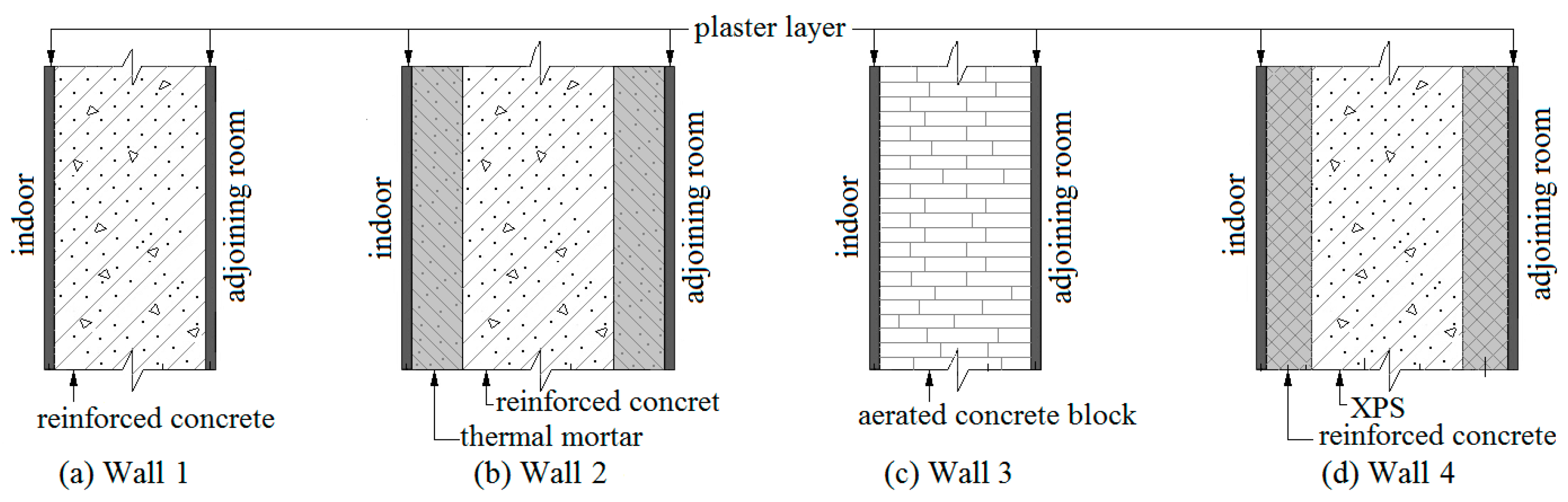
Four different configurations of internal walls commonly used in the HSCW zone are considered in this paper. A detailed schematic of internal wall configurations is shown in Figure 2. Figure 2a shows the Wall 1 containing thermal mass layer of 0.2 m reinforced concrete and 0.015 m plaster layers. Figure 2b shows the Wall 2, which consists of thermal mass layer of 0.2 m reinforced concrete, 0.03 m insulation layers of thermal mortar and 0.015 m plaster layers. Figure 2c shows a lightweight wall (Wall 3), which contains base wall layer of 0.2 m aerated concrete block and 0.015 m plaster layers. Figure 2d shows the Wall 4 containing thermal mass layer of 0.2 m reinforced concrete, insulation layers of 0.02 m XPS board and 0.015 m plaster layers. Thermal properties of the construction materials are given in

Table 1. Thermo-physical properties of building construction materials [5].

Material	Density ρ (kg/m3)	Specific Heat Capacity c [J/(kg⋅°C)]	Thermal Conductivity λ [W/(m⋅°C)]	Thermal Storage S [W/(m2⋅°C)]	Thermal Diffusivity α [m2/s]
Plaster layer	1700	1050	0.87	10.75	4.87 × 10−7
Reinforced concrete	2500	920	1.74	17.2	7.57 × 10−7
Thermal mortar	600	1050	0.18	2.87	2.86 × 10−7
Aerated concrete block	700	1050	0.18	3.10	2.45 × 10−7
XPS	35	1380	0.036	0.32	7.45 × 10−7

.

The thermal resistance and thermal diffusivity of the four walls are also given in

Table 2. Thermal resistance and thermal diffusivity of walls.

Internal Wall Configuration	Thermal Resistance R [m2⋅°C/W]	Thermal Diffusivity α [m2/s]
Wall 1	0.15	6.89 × 10−7
Wall 2	0.48	3.16 × 10−7
Wall 3	1.15	2.30 × 10−7
Wall 4	1.26	1.12 × 10−7

to better understand the heat conduction and storage process of walls.

Due to the effect of the thermal bridge, the heat transfer of connections between external and internal walls as well as the floor is a three-dimensional unsteady process. The heat transfer through the external wall is considered to be one-dimensional along the x-axis away from the connectors. For this reason, the envelopes of 0.5 m height in the four adjoining rooms on the directions of ±y, ±z based on the investigated room are also contained in the computational domain (seen in Figure 1). Moreover, the cross-sectional planes of envelope in the adjoining rooms are adiabatic surfaces.

The indoor thermal comfort environment is achieved by operating individual heating facilities with 600 m³/h supply air volume. The velocity of the air inlet is 2.38 m/s. The heating device is operated with high running power (3,500 W added with additional 1000 W electric auxiliary heat) when the average room temperature is lower than 18 °C. When the indoor air temperature rises to 20 °C, the running power of the heating device drops to 1800 W, and then the air temperature will decrease. Based on this system, the indoor air temperature varies between 18 and 20 °C.

2.2. Governing Equations

The airflow and temperature distribution in the room are set to maintain conservation laws of mass, momentum and energy. The airflow is simulated as unsteady state, incompressible, and turbulent. Based on the above assumptions, the governing time-averaged equations are given by [14]:

$$\frac{\partial u_{\mathrm{i}}}{\partial x_{\mathrm{i}}}=0$$

(1)

$$\frac{\partial u_{\mathrm{i}}}{\partial t}+\frac{\partial \left(u_{\mathrm{i}}{u}_{\mathrm{j}}\right)}{\partial x_{\mathrm{j}}}=-\frac{1}{\rho }\frac{\partial p}{\partial x_{\mathrm{i}}}+\frac{\partial }{\partial x_{\mathrm{j}}}\left(\nu \frac{\partial u_{\mathrm{i}}}{\partial x_{\mathrm{j}}}-\overline{{u^{\prime }}_{\mathrm{i}}{u^{\prime }}_{\mathrm{j}}}\right)$$

(2)

$$\frac{\partial \left(C_{\mathrm{p}}T\right)}{\partial t}+\frac{\partial \left(C_{\mathrm{p}}T{u}_{\mathrm{i}}\right)}{\partial x_i}=\frac{\partial }{\partial x_{\mathrm{j}}}\left[\left(\frac{\lambda }{\rho }+\frac{C_{\mathrm{p}}{\nu }_{\mathrm{t}}}{{Pr}_{\mathrm{t}}}\right)\frac{\partial T}{\partial x_{\mathrm{j}}}\right]$$

(3)

$$-\overline{{u^{\prime }}_{\mathrm{i}}{u^{\prime }}_{\mathrm{j}}}={\nu }_{\mathrm{t}}\left(\frac{\partial u_{\mathrm{i}}}{\partial x_{\mathrm{j}}}+\frac{\partial u_{\mathrm{j}}}{\partial x_{\mathrm{i}}}\right)-\frac{2}{3}k{\delta }_{\mathrm{i}\mathrm{j}}$$

(4)

$${\nu }_{\mathrm{t}}=C_{\mu }\frac{k^2}{\epsilon }$$

(5)

where x_i represents the Cartesian coordinates while the subscripts i and j range between 1 and 3, separately, refer to the (x, y, z) directions in space. The term u_i is the velocity of component i. p and T are the pressure and temperature, respectively. ρ and λ are the air density and thermal conductivity, respectively. ν is the kinematic viscosity, ν_t is the turbulent eddy viscosity, k is turbulent kinetic energy, and δ_ij is the Kronecker delta (i = j, δ_ij = 1; i ≠ j, δ_ij = 0).

The renormalization group (RNG) k-ε turbulence model is used to simulate the three-dimensional turbulent airflow, as it has been shown to accurately describe the flow field of the near wall region and relatively better predict of the indoor environment than the standard k-ε model by introducing an additional term in the ε-equation [15,16,17].

The transfer equations of turbulent kinetic energy k and turbulence dissipation rate ε are given by:

$$\frac{\partial k}{\partial t}+\frac{\partial }{\partial x_i}\left(k{u}_{\mathrm{i}}\right)=\frac{\partial }{\partial x_{\mathrm{j}}}\left[\left(\nu +\frac{{\nu }_{\mathrm{t}}}{{\sigma }_{\mathrm{k}}}\right)\frac{\partial k}{\partial x_{\mathrm{j}}}\right]-\overline{{u^{\prime }}_{\mathrm{i}}{u^{\prime }}_{\mathrm{j}}}\frac{\partial u_{\mathrm{j}}}{\partial x_{\mathrm{i}}}-\epsilon$$

(6)

$$\frac{\partial \epsilon }{\partial t}+\frac{\partial }{\partial x_{\mathrm{i}}}\left(\epsilon u_{\mathrm{i}}\right)=\frac{\partial }{\partial x_{\mathrm{j}}}\left[\left(\nu +\frac{{\nu }_{\mathrm{t}}}{{\sigma }_{\epsilon }}\right)\frac{\partial \epsilon }{\partial x_{\mathrm{j}}}\right]-C_{1\epsilon }\frac{\epsilon }{k}\overline{{u^{\prime }}_{\mathrm{i}}{u^{\prime }}_{\mathrm{j}}}\frac{\partial u_{\mathrm{j}}}{\partial x_{\mathrm{i}}}-C_{2\epsilon }^{\ast }\frac{{\epsilon }^2}{k}$$

(7)

$$C_{2\epsilon }^{\ast }=C_{2\epsilon }+\frac{C_{\mu }\rho {\eta }^3\left(1-\eta /{\eta }_0\right)}{1+\zeta {\eta }^3}$$

(8)

where η = S (k/ε) is the ratio between the time scales of the turbulence and the mean flow, S is the coefficient of surface tension and is defined by $S=\sqrt{2S_{\mathrm{i}\mathrm{j}}{S}_{\mathrm{i}\mathrm{j}}}$, $S_{\mathrm{i}\mathrm{j}}=\left(\partial u_{\mathrm{i}}/\partial x_{\mathrm{j}}+\partial u_{\mathrm{j}}/\partial x_{\mathrm{i}}\right)/2$. The constants appearing in the RNG k-ε model are: C_μ = 0.0845, C_1ε = 1.42, C_2ε = 1.68, σ_k = σ_ε = 0.7178, ζ = 0.012, η₀ = 4.38.

To observe the dynamic heat transfer process in envelope, a three-dimensional system of wall with thickness direction x, width direction y and height direction z is established (see Figure 3a). δ, W and H are the thickness, width, and height of the wall, respectively.

The heat transfer across the wall is described in the following equation [18,19]:

$$\frac{\partial T_{\mathrm{s}}}{\partial \mathrm{t}}=\frac{{\lambda }_{\mathrm{s}}}{{\rho }_{\mathrm{s}}{C}_{\mathrm{s}}}\left[\frac{\partial }{\partial x}\left(\frac{\partial T_{\mathrm{s}}}{\partial x}\right)+\frac{\partial }{\partial y}\left(\frac{\partial T_{\mathrm{s}}}{\partial y}\right)+\frac{\partial }{\partial z}\left(\frac{\partial T_{\mathrm{s}}}{\partial z}\right)\right]$$

(9)

Convective heat transfer boundary conditions are adopted on the wall’s inner and outer surfaces. For the inner surface, it is expressed as:

$${-{\lambda }_{\mathrm{s}}\frac{\partial T_{\mathrm{s}}}{\partial x}|}_{x=0}=h_{\mathrm{i}}(T_{x=0}-T_{\mathrm{i}})$$

(10)

For the outer surface, it can be expressed as:

$${-{\lambda }_{\mathrm{s}}\frac{\partial T_{\mathrm{s}}}{\partial x}|}_{x=\delta }=h_{\mathrm{o}}(T_{\mathrm{a}}-T_{x=\delta })$$

(11)

Moreover, adiabatic boundary conditions are used on the cross-sectional planes (y = 0 and y = W, z = 0 and z = H) of the envelope [20]:

$${\frac{\partial T_{\mathrm{s}}}{\partial y}|}_{y=0,W}={\frac{\partial T_{\mathrm{s}}}{\partial z}|}_{z=0,H}=0$$

(12)

where ρ_s and λ_s are the density and thermal conductivity of the wall, respectively. T_a refers to the temperature of the surrounding air (i.e., the outdoor air or the adjoining air). T_i is the indoor air temperature. h_i and h_o are the heat transfer coefficients of inner and outer surfaces of walls, respectively.

2.3. Numerical Aspects and Boundary Conditions

The commercial program of ANSYS 6.3.26 with the finite volume method is employed to solve the three-dimensional numerical simulations. To improve the accuracy of the numerical simulations, second-order discretization schemes are applied to the momentum, turbulent kinetic energy, and turbulent dissipation rate equations. Semi-Implicit Method for Pressure Linked Equations (SIMPLE) algorithm is used to evaluate pressure-velocity coupling in the continuity equations. Meanwhile, the standard wall-function method is applied to model the near wall regions with low Reynolds number [21].

According to the “Design standard for energy efficiency of residential buildings in hot summer and cold winter zone” (JGJ 134-2010) [22], the cold air infiltration is 1 h⁻¹. The heat transfer coefficient for the window should be less than 4.7 W/(m²⋅°C), and the window: external wall area ratio should be less than 0.4 (north-facing) and 0.45 (south-facing), respectively. Thus, the area of window in the computational model is 3 m², and the heat transfer coefficient of window is 3.0 W/(m²⋅°C).

At the inlet of the computational domain, uniform velocity and temperature are imposed, and the inlet values of turbulent kinetic energy (k₀) and dissipation rate (ε₀) profiles [23] are set as follows:

$$T_{\mathrm{u}}=0.16{\left({Re}_{\mathrm{L}}\right)}^{-1/8}$$

(13)

$${\epsilon }_0=C_{\mu }^{3/4}\frac{k^{3/2}}{l}$$

(14)

where V, T_u and Re_L, respectively, denote the mean velocity, the turbulence intensity, and the Reynolds number at the inlet. l is a length scale defined as l = 0.07 L, where L is the hydraulic diameter at the inlet. Furthermore, outflow boundary condition is applied at the outlet of the computational domain and non-slip conditions are imposed on the inner surfaces of solid walls.

2.4. Grid Independency

The computational domain is discretized with tetrahedral elements, while non-uniform computational grids are used for the present simulation. To describe the heat transfer and flow status more accurately, grids are further refined near walls, inlet and outlet, while relatively coarse grids are used for zones away from solid surfaces. The expansion rate between two consecutive cells is no more than 1.12.

To ensure the first numerical point is located inside the logarithmic layer, the variable y⁺, termed as the dimensionless wall distance, is controlled in the range of 90~220, satisfy the requirement range of 30 ≤ y⁺ ≤ 300 for RNG k-ε model using standard wall functions [24].

$$y^{+}=\frac{y}{\nu }\sqrt{\frac{{\tau }_w}{\rho }}$$

(5)

where, y is the vertical distance from wall to the first cell center. ν is the kinematic viscosity. τ_w is the wall shear stress.

Grid independency is carried out to achieve converged results of the simulations. A set of pre-simulations are carried out to check the same physical parameters by using different grid densities (coarse, normal, and fine), and the grid number is increased until the numerical results will not be affected by the grid size. In this study, the root-mean-square error in the temperature, shown in Equation (16), ε_r,m,s of less than 2% is used as the criterion for grid independence [25].

$${\epsilon }_{r,m,s}=\sqrt{\frac{1}{N}{\displaystyle {\sum }_1^N{\left(\frac{T_{i,f}-T_{i,c}}{T_r}\right)}^2}}$$

(16)

where, T_i,f is the temperature in the former grid number, T_i,c is the temperature in the current grid number, the subscript i represents the ith sampling point, T_r = 19 °C is the reference temperature, and N is the number of the examined sample points. Based on the different configurations of building envelope, the resulting unstructured grid numbers of 4.03~5.02 million are used for the simulations.

2.5. Model Validation

Validation exercises were performed to ensure the reliability of the results from the CFD simulations. The temperature fields in a test chamber were investigated by experimental and numerical simulation. Figure 4 gives the detailed arrangement of the test system.

The experiment was carried out in an environment chamber with dimensions of 3.6 × 3.0 × 2.6 m (L × W × H), which is placed in a large laboratory, as shown in Figure 4a. The walls of the chamber were made of 0.01 m thickness colored steel plates which were hollow and filled with 0.07 m thickness insulated rock wool. The heat transfer coefficient of the envelopes was about 0.9 W/(m²⋅°C). The dimension of door was 0.7 m × 2 m. The door was open, and the area of which was covered with plastic film. The fresh air ratio was regulated to 10%, and the condition of slightly positive pressure was maintained in the chamber during the experiment. Two boxes with dimensions of 0.5 m × 0.3 m × 0.28 m (see Figure 4b), containing mixture of dry sand and steel reinforcing rods were placed at the floor near one internal wall. Moreover, the mass ratio of the dry sand to the steel reinforcing rods was about 0.91, and the thermal conductivity of the mixture was 0.7 (W/(m⋅°C)).

The air conditioning system was used to warm the chamber. The supply velocity and temperature of the warm air inlet is 1.62 m/s and 36.9 °C, respectively. The air inlet was placed at the height of 0.15 m with the dimension of 0.3 m × 0.1 m. The exhaust device was mounted at the center of the ceiling with the dimension of 0.3 m × 0.2 m.

The temperature was measured by Type-K thermocouples with an accuracy of ±0.1 °C. The temperature of each wall was measured at the central point by thermocouples. Because the walls were made of colored steel plates with uniform temperature distribution, the value of the points can represent the corresponding surface temperature. In addition, four thermocouples were placed uniformly in each mixture, the turn of which from external to internal side is measuring point 1, 2, 3 and 4. The distribution of four measuring points in the mixture is shown in Figure 4c. All the thermocouples were covered with aluminum foil tape to minimize radiation effects.

Before the tests, the air temperature of the chamber and the outside laboratory had been kept at 10 °C for two hours by adequately ventilating. Then the air conditioning system was operated, and the air temperature of the outside laboratory was kept at 10 ± 1 °C during the experiment.

Moreover, the RNG k-ε model was verified by experimental data to simulate the thermal performance of heating room and the dynamic thermal behavior of thermal mass. Figure 5 gives the comparisons of temperature distribution of the mixture 1 between CFD simulations and the experimental data.

Figure 5a–d indicates that the numerical predictions of the temperature distribution in Mixture 1 are in good agreement with the measured results. The temperature difference of Point 2 is the maximum of the four points, while which is less than 0.3 °C. Moreover, the temperature difference of the other three points is less than 0.1 °C. Hence, it can be concluded that the numerical simulation used in the present study is appropriate for simulating the temperature fields in the heating room.

2.6. Study Cases

In the present study, five intermittent heating durations have been considered, ranging from 0.5 h to 8 h, according to the occupants’ behavior in residential buildings [26]. A heating cycle contains heating duration and heating cessation duration, in which the heating cessation duration is 2 h. The results of four heating cycles is given in this paper. The detailed heating operation cases are summarized in

Table 3. Information of operation cases.

Operation Case	Heating Duration per Operation τo (h)	Hours Contained in a Heating Cycle τ (h)
Cτ=0.5	0.5 h	2.5 h
Cτ=1	1 h	3 h
Cτ=2	2 h	4 h
Cτ=4	4 h	6 h
Cτ=8	8 h	10 h

.

3. Results and Discussion

3.1. Comparison of Surface Temperature of Four Internal Wall Configurations

To observe the dynamic thermal behavior of four internal walls for different heating durations, Figure 6 shows the variations of inner surface temperature T_in,i of the internal walls, taking heating duration of 1 and 8 h as examples.

It is found in Figure 6 that at the starting time of heating cycle, the T_in,i of Wall 4 (insulted with XPS) is increasing rapidly at the beginning of the heating period, and then fluctuates at 16 °C, approaching the indoor air temperature T_i (18 °C to 20 °C). However, T_in,i of the other three internal walls increases slowly and is obviously lower than the T_in,i of Wall 4 during the whole heating period. Once the heating device is shut off, T_in,i drops sharply for Wall 4, but drops slowly for the other three internal walls. The reason is the heat capacity of the inner layer of Wall 4 is the lowest, which leads to nearly no time lag between changes of T_in,i and T_i (indoor air temperature).

Comparing Figure 6a,b, it can be seen that the T_in,i of Wall 2 is equal to that of Wall 3 during heating period in Figure 6a. However, when it comes to the longer heating duration, as shown in Figure 6b, significant temperature difference is found between the inner surface of Wall 2 and Wall 3. This is because the thermal resistance of Wall 2 is smaller than Wall 3, which leads to more heat transferring to the inside of Wall 2 with the heating duration increases.

The internal walls absorb and store heat from indoor air during the heating period. Then, some heat transfers through the internal walls, which leads to the fluctuation of surface temperature of internal walls close to the adjoining room. The outer surface temperature (T_in,o) of internal walls close to the adjoining room is shown in Figure 7 for short and long heating duration.

As shown in Figure 7a, the T_in,o of four internal walls is similar to each other and close to the adjoining air temperature. It indicates that almost all the heat absorbed by the inner layer of internal walls is stored and little energy transfer to the outer surface of internal walls for short heating duration.

An apparent increase of T_in,o of four internal walls is found in Figure 7b for long heating duration, and the difference of T_in,o between four walls increases with the increase of heating duration. The raise of T_in,o ranks from high to low with the configuration of Wall 1, Wall 4, Wall 2, and Wall 3. This is dependent on the heat capacity of inner layer and thermal resistance of four internal walls. T_in,o of the Wall 1 is the highest due to its higher thermal capacity and lower thermal resistance.

3.2. Comparison of Surface Heat Flow of Four Internal Walls

Figure 8 shows the variation of inner surface heat flow (q_i) of four internal walls with time under short and long heating durations.

As shown in Figure 8a, the inner surface heat flow q_i of Wall 4 is the lowest of the four walls, and the heat flow q_i of the other three walls are similar to each other during heating period. This is because Wall 4 gives the smallest temperature difference between the inner surface and indoor air, and hence the smallest heat flow q_i. It can also be seen from Figure 8a that the internal walls release heat to the indoor air during heating cessation period, and the heat flow achieves a similar effect by the configuration of internal walls.

The results in Figure 8b indicate that Wall 4 still demonstrates the smallest heat flow among the four internal wall types, which is consistent with the situation presented in Figure 8a. However, the heat flow of Wall 3 drops gradually with the heating duration and is almost equal to the q_i of Wall 4. This is because of the similar temperature different between indoor air and inner surface temperature of Wall 3 and Wall 4.

To evaluate the heat transferring to the adjoining room, the variation of the heat flow q_o between outer surface (close to the adjoining room) of internal wall and adjoining air are shown in Figure 9.

It can be observed from Figure 9a that the heat flow q_o of four internal walls is always small for heating case C_τ=1 (less than 5 W), and the difference of q_o between four walls is slight. With the increase of heating duration, the heat flow q_o increases obviously (as shown is Figure 9b). Moreover, a significant difference of q_o between four walls is observed. This is because of the temperature difference of outer surface between the four internal walls.

The results in Figure 9b also shows that the heat flow is nearly zero when the heating duration is less than 5 h. It means the process of heat absorption and storage of internal walls lasts 5 h before heat transferring to the adjoining room, no matter what the configuration of internal wall is.

3.3. Threshold Value of Daily Operation Hours Under Four Internal Wall Configurations

It is obvious that the extent of building walls heated by indoor air is different under various heating durations, which will lead to different heating loads of the unit floor area per unit time. Therefore, the heating load index Q_i, as expressed in Equation (17), is introduced to analyze the characteristics of the heating load during the heating period. Also, the increasing rate η, as expressed in Equation (18), is employed to compare the heating load index between intermittent heating mode and continuous heating mode.

$$Q_{\mathrm{i}}={\displaystyle \underset{0}{\overset{{\tau }_o}{\int }}pd{\tau }_{\mathrm{o}}}/(F\times {\tau }_{\mathrm{o}})$$

(17)

$$\eta =\frac{Q_{\mathrm{i},\mathrm{m}}-Q_{\mathrm{i},\mathrm{c}}}{Q_{\mathrm{i},\mathrm{c}}}\times 100\%$$

(18)

where p is the running power of heating device. τ_o is the heating duration. F is the floor area of the investigated room. Q_i,m is the heating load index for intermittent heating. Q_i,c is the heating load index for 24 h continuous heating (C_con).

Figure 10 demonstrates the effect of intermittent heating duration on the heating load index Q_i for four internal wall configurations, and the case of 24 h (C_con) heating duration is also given.

Figure 10 shows that Q_i of intermittent heating is significantly larger than that of C_con. This is because the inner layer of walls release heat during heating cessation time, which leads to more energy being required to heat the inside layer of the walls at the next heating cycle for intermittent heating. Compared with Figure 10a–d, it can be found that the heating load index with the same heating duration drops in turn under the Wall 1, Wall 2, Wall 3, and Wall 4. The heating load index depends on the heat convection between the inner surface of walls and indoor air. Wall 1 gives the largest temperature difference between the inner surface of walls and indoor air. Therefore, the largest Q_i is obtained by Wall 1.

It can be seen in Figure 10a that the increasing rate η ranges from 31.58% to 76.35% for five heating durations. Moreover, the heating cessation time ratio of C_τ=8 is 20%, while the increasing rate η is 31.58%, which is larger than 20%. This indicates that the daily heating load of heating time ratio 19.2/24 is larger than that of 24 h continuous heating and a threshold value of daily operation hour exists for intermittent heating mode. By comparing Figure 10a–d, it also can be seen that with various internal wall configurations, the increasing rate η is different. This will lead to various threshold values of daily operation hours.

The daily heating load is calculated by Equation (19):

$$Q=Q_i\times \frac{24{\tau }_{\mathrm{o}}}{\tau }$$

(19)

where τ is the hours contained in a heating cycle (see Table 3).

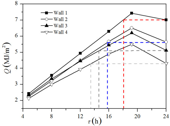
The variation of daily heating load (Q) with operation hour for internal wall configurations is shown in Figure 11.

As illustrated in Figure 11, the daily heating load (Q) is increasing continuously at first and then decreasing linearly with the operation hour per day. Comparing the heating load of intermittent (Q_m) and 24 h continuous heating (Q_c), Q_m is larger than Q_c when the heating time ratio is 19.2/24 and Q_m is smaller than Q_c when the heating time ratio is 12/24.

The threshold value of operation hours 18.04 h, 15.80 h, 14.59 h and 13.46 h, respectively, for Wall 1, Wall 2, Wall 3, and Wall 4. The threshold value of Wall 1 is 18.04 h, which is close to 18 h obtained in the research [8]. This is because the thermal performance of envelope investigated in two papers is similar. With the operation hours lower than the threshold value, the daily heating load is clearly less than that of continuous heating. Nevertheless, it seems to be more economical to use continuous heating mode when the operation hour is more than the threshold value.

It also can be found that the variation of heating load index with internal wall configurations is consistent with the variation of threshold value with internal wall configurations, which drops in turn under Wall 1, Wall 2, Wall 3, and Wall 4. This means that with the increase of insulation level of the internal wall, the optimum heating duration decreases.

4. Conclusions

The relatively low outdoor temperature and absence of district heating leads to the intermittent heating operation mode in the HSCW climate zone of China. More heat is absorbed by building walls during the heating period due to the heat release and storage of the internal wall, while it is not required for continuous heating mode. Therefore, the heating load of the unit floor area per unit time for intermittent heating mode is larger than that of continuous heating mode. This means that the daily heating load of intermittent heating will be larger than that of continuous heating, and a threshold value of daily operation hours occur for intermittent heating.

In the present work, a three-dimensional simulation method is established to study the heating load of buildings with different intermittent heating duration and configuration of internal walls. The threshold value of daily operation hours is analyzed under four configurations of internal walls by comparing the heating load of continuous and intermittent heating. Thorough experiments on temperature distributions of thermal mass are carried out to validate the simulation model.

In the intermittent heating room, the temperature of building envelope increases by storing energy during heating period, and the inside layer cools to a lower temperature during heating cessation period. As a result, more energy is used to heat the inside layer of the walls at the starting time of the heating cycle. This leads to a lager heating load index for intermittent heating system than continuous heating system with increasing rate ranging from 31.58% to 152.63%.

By comparing the daily heating load with operation hours, it is found that the daily heating load increases to a peak value as the operation hours increase, and then starts to decrease. This indicates that the threshold value of operation hours is 18.04 h, 15.80 h, 14.59 h and 13.46 h for four internal wall configurations, respectively. Moreover, with the increase of insulation level of internal walls, the optimum heating duration decreases. In addition, the results indicate that it is more economical to use continuous heating when the daily operation hours are more than the threshold values.

It should be noted that the threshold value of daily operation hours given in this paper is obtained according to the present situation of heating in the HSCW zone. However, the heating duration per day and the amount of heated rooms are increasing with the rapid growth of the economy and continuous increase of disposable personal income. This leads to a higher average air temperature of adjoining rooms; thus, a smaller threshold value of daily operation hours is obtained, which will be discussed in future works. Moreover, just four configurations of internal wall commonly used in the HSCW zone are investigated in this paper, and the threshold value of daily operating hours varies for other configurations of the internal wall.

References

- Yoshino, H.; Yoshino, Y.; Zhang, Q.; Mochida, A.; Li, N.; Li, Z.; Miyasaka, H. Indoor thermal environment and energy saving for urban residential buildings in China. Energy Build. 2006, 38, 1308–1319. [Google Scholar] [CrossRef]
- Hu, T.; Yoshino, H.; Jiang, Z. Analysis on urban residential energy consumption of Hot Summer & Cold Winter Zone in China. Sustain. Cities Soc. 2013, 6, 85–91. [Google Scholar]
- Guo, S.; Yan, D.; Peng, C.; Cui, Y.; Zhou, X.; Hu, S. Investigation and analyses of residential heating in the HSCW climate zone of China: Status quo and key features. Build. Environ. 2015, 94, 532–542. [Google Scholar] [CrossRef]
- Yu, J.; Yang, C.; Tian, L. Low-energy envelope design of residential building in hot summer and cold winter zone in China. Energy Build. 2008, 40, 1536–1546. [Google Scholar] [CrossRef]
- Code for Thermal Design of Civil Building; The People’s Republic of China National Standard GB 50176-2016; China Architecture and Building Press: Beijing, China, 2016. (In Chinese)
- Yoshino, H.; Guan, S.; Lun, Y.F.; Mochida, A.; Shigeno, T.; Yoshino, Y.; Zhang, Q.Y. Indoor thermal environment of urban residential buildings in China: Winter investigation in five major cities. Energy Build. 2004, 36, 1227–1233. [Google Scholar] [CrossRef]
- Hu, S.; Yan, D.; Cui, Y.; Guo, S. Urban residential heating in hot summer and cold winter zones of China-Status, modeling, and scenarios to 2030. Energy Policy 2016, 92, 158–170. [Google Scholar] [CrossRef]
- Le, J.; Heiselberg, P. Energy flexibility of residential buildings using short term heat storage in the thermal mass. Energy 2016, 111, 991–1002. [Google Scholar]
- Badran, A.A.; Jaradat, A.W.; Bahbouh, M.N. Comparative study of continuous versus intermittent heating for local residential building: Case studies in Jordan. Energy Convers. Manag. 2013, 65, 709–714. [Google Scholar] [CrossRef]
- Tsilingiris, P.T. Wall heat loss from intermittently conditioned space-The dynamic influence of structural and operational parameters. Energy Build. 2006, 38, 1022–1031. [Google Scholar] [CrossRef]
- Meng, X.; Luo, T.; Gao, Y.; Zhang, L.; Huang, X.; Hou, C.; Shen, Q.; Long, E. Comparative analysis on thermal performance of different wall insulation forms under the air-conditioning intermittent operation in summer. Appl. Therm. Eng. 2018, 130, 429–438. [Google Scholar] [CrossRef]
- Zhang, L.; Luo, T.; Meng, X.; Wang, Y.; Hou, C.; Long, E. Effect of the thermal insulation layer location on wall dynamic thermal response rate under the air-conditioning intermittent operation. Case Stud. Therm. Eng. 2017, 10, 79–85. [Google Scholar] [CrossRef]
- Yuan, L.; Kang, Y.; Wang, S.; Zhong, K. Effects of thermal insulation characteristics on energy consumption of buildings with intermittently operated air-conditioning systems under real time varying climate conditions. Energy Build. 2017, 155, 559–570. [Google Scholar] [CrossRef]
- ANSYS FLUENT, 14.0 Theory Guide; ANSYS: Canonsburg, PA, USA, 2011.
- Gebremedhin, K.G.; Wu, B.X. Characterization of flow field in a ventilation space and simulation of heat exchange between cows and their environment. J. Therm. Biol. 2003, 28, 301–319. [Google Scholar] [CrossRef]
- Coussirat, M.; Guardo, A.; Jou, E.; Egusquiza, E.; Cuerva, E.; Alavedra, P. Performance and influence of numerical sub-models on the CFD simulation of free and forced convection in double-glazed ventilated façades. Energy Build. 2008, 40, 1781–1789. [Google Scholar] [CrossRef]
- Rohdin, P.; Moshfegh, B. Numerical predictions of indoor climate in large industrial premises. A comparison between different k-ε models supported by filed measurements. Build. Environ. 2007, 42, 3872–3882. [Google Scholar] [CrossRef]
- Meng, X.; Yan, B.; Gao, Y.; Wang, J.; Zhang, W.; Long, E. Factors affecting the in situ measurement accuracy of the wall heat transfer coefficient using the heat flow meter method. Energy Build. 2015, 86, 754–765. [Google Scholar] [CrossRef]
- Ozel, M. Thermal performance and optimum insulation thickness of building walls with different structure materials. Appl. Therm. Eng. 2011, 31, 3854–3863. [Google Scholar] [CrossRef]
- Casalegno, A.; Antonellis, S.D.; Colombo, L.; Rinaldi, F. Design of an innovative enthalpy wheel based humidification system for polymer electrolyte fuel cell. Int. J. Hydrogen Energy 2011, 36, 5000–5009. [Google Scholar] [CrossRef]
- Ye, X.; Kang, Y.; Zuo, B.; Zhong, K. Study of factors affecting warm air spreading distance in impinging jet ventilation rooms using multiple regression analysis. Build. Environ. 2017, 120, 1–12. [Google Scholar] [CrossRef]
- Ministry of Housing and Urban-Rural Development of the People’s Republic of China. Design Standard for Energy Efficiency of Residential Buildings in Hot Summer and Cold Winter Zone (JGJ134-2010); China Architecture and Building Press: Beijing, China, 2010. (In Chinese)
- ANSYS FLUENT 14.0 User’s Guide; ANSYS: Canonsburg, PA, USA, 2011.
- Hussain, S.; Oosthuizen, P.H.; Kalendar, A. Evaluation of various turbulence models for the prediction of the airflow and temperature distributions in atria. Energy Build. 2012, 48, 18–28. [Google Scholar] [CrossRef]
- Ye, X.; Zhu, H.; Kang, Y.; Zhong, K. Heating energy consumption of impinging jet ventilation and mixing ventilation in large-height space: A comparison study. Energy Build. 2016, 130, 697–708. [Google Scholar] [CrossRef]
- Lin, B.; Wang, Z.; Liu, Y.; Zhu, Y.; Ouyang, Q. Investigation of winter indoor thermal environment and heating demand of urban residential buildings in China’s hot summer-cold winter climate region. Build. Environ. 2016, 101, 9–18. [Google Scholar] [CrossRef]
Figure 1.
Schematic of the room: (a) three-dimensional schematic of the room model; (b) side view (plane y-z) of the model.
Figure 2.
Sections of four kinds of internal wall structures.
Figure 3.
Simulation model of internal wall: (a) three-dimensional schematic of internal wall; (b) heat transfer boundary conditions on the wall surfaces.
Figure 4.
Schematic of the experimental system: (a) layout of the laboratory, (b) dry sand and steel reinforcing rods in the boxes, (c) measuring points in the mixture.
Figure 5.
Validation of temperature distribution in a thermal mass: (a) Point-1; (b) Point-2; (c) Point-3; (d) Point-4.
Figure 6.
Variations of inner surface temperature Tin,i of the internal walls with time: (a) Cτ=1, (b) Cτ=8. Note: the light gray zone in Figure 6 represents the heating cessation period.
Figure 7.
Variations of outer surface temperature Tin,o of the internal walls with time: (a) Cτ=1, (b) Cτ=8.
Figure 8.
Variation of inner surface heat flow qi of four internal walls with time: (a) Cτ=1, (b) Cτ=8.
Figure 9.
Variation of outer surface heat flow qo of four internal walls with time: (a) Cτ=1, (b) Cτ=8.
Figure 10.
Variations of Qi and η with operation cases: (a) Wall 1, (b) Wall 2, (c) Wall 3, (d) Wall 4.
Figure 11.
Variations of daily heating load (Q) with operation hour.