A Stochastic Bulk Damage Model Based on Mohr-Coulomb Failure Criterion for Dynamic Rock Fracture

Department of Mechanical Aerospace and Biomedical Engineering, University of Tennessee Space Institute, Tullahoma, TN 37388, USA
*
Author to whom correspondence should be addressed.
Appl. Sci. 2019, 9(5), 830; https://doi.org/10.3390/app9050830
Submission received: 10 February 2019
/
Accepted: 20 February 2019
/
Published: 26 February 2019
(This article belongs to the Special Issue Computational Methods for Fracture)
Abstract
:We present a stochastic bulk damage model for rock fracture. The decomposition of strain or stress tensor to its negative and positive parts is often used to drive damage and evaluate the effective stress tensor. However, they typically fail to correctly model rock fracture in compression. We propose a damage force model based on the Mohr-Coulomb failure criterion and an effective stress relation that remedy this problem. An evolution equation specifies the rate at which damage tends to its quasi-static limit. The relaxation time of the model introduces an intrinsic length scale for dynamic fracture and addresses the mesh sensitivity problem of earlier damage models. The ordinary differential form of the damage equation makes this remedy quite simple and enables capturing the loading rate sensitivity of strain-stress response. The asynchronous Spacetime Discontinuous Galerkin (aSDG) method is used for macroscopic simulations. To study the effect of rock inhomogeneity, the Karhunen-Loeve method is used to realize random fields for rock cohesion. It is shown that inhomogeneity greatly differentiates fracture patterns from those of a homogeneous rock, including the location of zones with maximum damage. Moreover, as the correlation length of the random field decreases, fracture patterns resemble angled-cracks observed in compressive rock fracture.
1. Introduction
Interfacial, particle, and bulk or continuum models form the majority of approaches used for failure analysis of quasi-brittle materials at continuum level. Interfacial models directly represent sharp fractures in the computational domain. Some examples are Linear Elastic Fracture Mechanics (LFEM), cohesive models [1,2], and interfacial damage models [3,4,5,6,7]. Since cracks are explicitly represented, interfacial methods are deemed accurate when crack propagation is the main mechanism of material failure. However, external criteria are needed for crack nucleation and propagation (direction and extension). Moreover, accurate representation of arbitrary crack directions can be cumbersome in computational settings. Mesh adaptive schemes [8,9,10], eXtended Finite Element Methods (XFEMs) [11,12,13], and Generalized Finite Element Methods (GFEMs) [14,15] address this problem to some extend. However, for highly dynamic fracture simulations and fragmentation studies, even these methods have challenges in accurate modeling of the fracture pattern. Particle methods such as Peridynamics [16,17,18] have been successfully used to model highly complex fracture patterns that are encountered in dynamic (rock) fracture. They model continua as a collection of interacting particles.
Bulk or continuum damage models approximate the effect of material microstructural defects and their evolution, e.g., microcrack nucleation, propagation, and coalescence, through the evolution of a damage parameter. Due to the implicit representation of microcracks and other defects, bulk damage models are more efficient than interfacial and especially particle methods. In addition, damage pattern is obtained as a part of the solution and no external criteria are needed for crack nucleation and propagation. Finally, since damage is a smooth field interpolated within finite elements, complex fracture patterns can be easily modeled by damage models, wherein the thickness of cracks is effectively regularized by the damage field.
Earlier bulk damage models, however, suffered from mesh sensitivity problem where the width of the localization and damaged region was proportional to element size; as a result, finer meshes resulted in a more brittle fracture response. This problem is related to the loss of ellipticity/hyperbolicity of the (initial) boundary value problem for the earlier formulations [19,20], and can be resolved by the introduction of an intrinsic length scale to the damage evolution formulation. In gradient-based models, this is achieved by adding higher order derivatives of the damage or strain fields to the damage evolution equation [21,22]. In nonlocal approaches, strain or damage field employed in a local damage formulation, is in turn computed over a neighborhood of finite size [23,24]. Finally, time-relaxed damage formulations possess an internal time parameter which through its interaction with elastic wave speeds introduce a finite length scale for the damage model in transient settings [25,26,27,28]. Related to these remedies is the phase field method which closely resembles a gradient-based damage model [29]. The sharper approximation of crack width is one of the main advantages of the phase field methods to gradient-based damage models [30].
We have presented a time-delay damage model for dynamic brittle fracture in [31]. The coupled elastodynamic-damage problem is solved by the asynchronous spacetime Discontinuous Galerkin (aSDG) method [32,33]. This damage model addresses the mesh sensitivity problem of the earlier damage models by the third approach discussed above, in that, damage evolution is governed by a time-delay model. In addition, the existence of a maximum damage evolution rate results in an increase in both the maximum attainable stress and toughness as the loading rate increases. This loading rate dependency of strength and toughness is experimentally verified; see for example [24,34]. Finally, the damage evolution law is an Ordinary Differential Equation in time. This greatly simplifies the damage model formulation and lends itself to the aSDG method; the aSDG method directly discretizes spacetime by elements that satisfy the causality constraint of the underlying hyperbolic problem being solved. The nonlocal damage models violate this causality constraint, whereas the majority of gradient-based damage models are not hyperbolic. In contrast, the time-delay damage model maintains the hyperbolicity of the elastodynamic problem. Besides, the ODE form of the governing equation greatly simplifies the application of initial and boundary conditions for the coupled problem.
The distribution of material defects at microstructure can have a great effect on macroscopic fracture response, particularly for quasi-brittle materials. Some examples are high variability in fracture pattern for samples with the same loading and geometry [35], high sensitivity of macroscopic strength and fracture toughness to microstructural variations [36], and the so-called size effect [37,38,39], i.e., the decrease of the mean and variations of fracture strength for larger samples. Weibull model [40,41] is one of the popular approaches for modeling the effect of defects in quasi-brittle fracture, particularly the size effect. We have used the Weibull model in the context of an interfacial damage model to capture statistical fracture response of rock, in hydraulic fracturing [42], fracture under dynamic compressive loading [43], and in fragmentation studies [44,45]. However, these models are computationally expensive due to the use of a sharp interfacial damage model.
In this manuscript, we propose a stochastic bulk damage model for rock fracture. There are two main differences to the damage model presented in [31]. First, in damage mechanics often only the spectral positive part of either strain or elastic stress tensor is used to drive damage accumulation. Moreover, upon full damage, only the negative part of the stress tensor is maintained in forming the effective stress. While these choices are appropriate for tensile-dominant fracture, they have some shortcomings for rock fracture under compressive loading. Specifically, using these models damage does not accumulate under compressive loading; even if it could, it would not have modeled the failure process as the effective stress remains the same as the elastic stress of the intact rock. Herein, we propose a new damage model based on the Mohr-Coulomb failure criterion and an effective stress that correctly represents rock failure in compression. Second, we employ a stochastic damage model wherein rock cohesion is treated as a random field. This aspect is important for the uniaxial compression examples considered, as due to the lack of macroscopic stress concentration points highly unrealistic fracture patterns will be obtained by using a homogeneous rock mass model. We note that the use of a bulk damage model makes the proposed approach significantly more efficient than the stochastic fracture problems [42,43,44,45] studies by the authors using an interfacial damage model.
The outline of the manuscript is as follows. The formulation of the stochastic damage model, its coupling to elastodynamic problem, and the aSDG method are discussed in Section 2. We use a dynamic uniaxial compressive example to demonstrate the effect of material inhomogeneity on fracture response in Section 3. Final conclusions are drawn in Section 4.
2. Formulation
The first three subsections are pertained to the formulation of damage model. In Section 2.1 the formulation of the damage force parameter based on the Mohr-Coulomb (MC) failure criterion and the damage evolution equation are provided. In Section 2.2 the coupling of elasticity and damage problems through the effective stress is described. Certain properties of the damage model are discussed in Section 2.3. A brief description of the aSDG method and the implementation of the damage model is provided in Section 2.4. Finally, the stochastic aspects of the damage model are explained in Section 2.5.
2.1. Bulk Damage Problem Description
2.1.1. Damage Driving Force
As will be discussed in Section 2.2, the damage parameter gradually reduces the elasticity stiffness in the process of material degradation. Damage evolution if generally driven by the strain field . For the remainder of the manuscript, we assume that the spatial dimension is two. The symmetric elastic stress tensor is defined as,
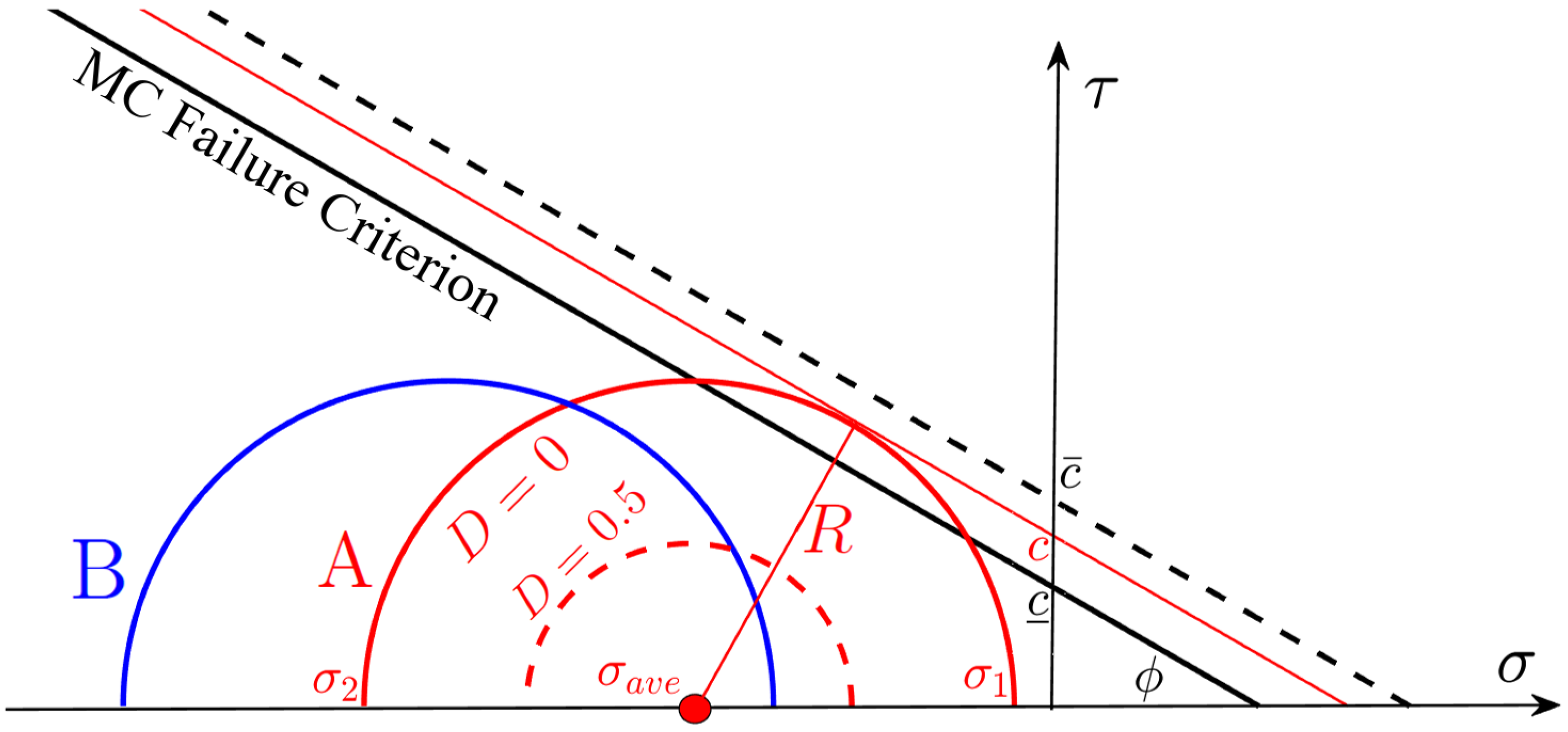
are the expressions of stress and strain tensors in global coordinate system and is the elasticity tensor. Instead of , damage evolution can be expressed in terms of . This is more suitable for rock fracture given that many known failure criteria such as Mohr-Coulomb (MC) or Hoek-Brown [46] are expressed in terms of the stress tensor. Figure 1 shows the Mohr-Coulomb failure criterion in terms of normal and shear traction components on a fracture surface. We employ the tensile positive convention for . The failure criterion is determined by the cohesion and friction angle , where k is the friction coefficient. In the figure, the Mohr circle for a stress tensor A (red semi-circle) corresponding to principal stresses is shown. Since only isotropic rocks are considered herein, and are assumed to be constant with respect to the orientation of principal stresses (with respect to the global coordinate system axes). We define the scalar stress as,
where as shown in Figure 1, c is the ordinate of the tangent line on the Mohr-circle with angle , and the radius R and average normal stress are given by,
Figure 1 shows two stress states. For the stress state B, the entire Mohr circle is below the failure criterion curve, thus no degradation is expected. For the stress state A, the Mohr circle expands beyond the failure criterion curve; in a binary intact and failed classification, this stress state would be considered failed. These stages correspond to and , respectively. Some specific strengths corresponding to the MC criterion are shown in Figure 2 and are given by,
As will become clear later, the damage model, regularizes the process of failure. Otherwise, failure for a stress state occurs instantaneously once MC criterion is satisfied; for example, when reaches (). To facilitate this, the damage force is defined as,
where corresponds to the ordinate of the upper MC line shown in dashed line in Figure 1. The brittleness factor defines a relation between the two MC lines through . In the absence of the damage model, complete failure occurs for any positive value of as the Mohr circle expands over the failure criterion. However, in the context of the damage model, corresponds to the quasi-static damage value for a given strain , which through (1) and (2) defines c. For example, for the strain (elastic stress) state A in Figure 1, .
2.1.2. Damage Evolution Law
The damage value can be taken to be equal to the damage force. However, this local definition of D has several shortcomings, as will be discussed below and in Section 2.3.2. We employ the time-delay model in [3,25] for damage evolution. The rate of damage evolution, , is given by,
where is a general source term for the evolution equation . This function can be calibrated from experimental strain-stress results, for example, for uniaxial tensile/compressive loading. The specific form of is taken from [3,47] as it is claimed to accurately model materials’ rate effect; cf. Section 2.3.2. In addition, is the relaxation time, a is the brittleness exponent, and is the Macaulay positive operator.
Albeit its simplicity, this evolution model incorporates several essential characteristics of real materials. First, we observe that the damage evolution is governed by the difference of damage D and damage force . The higher the difference, the higher the damage rate. Moreover, when , damage evolution terminates. That is, is the target damage value; if D is smaller than the target value, it evolves until it reaches . Second, damage cannot instantaneously reach given that is bound by the maximum damage rate . As will be discussed in Section 2.3.2, this results in the rate-sensitivity of strain-stress response. Third, the positive operator ensures that damage is a nondecreasing function in time (no material healing processes). Finally, Figure 3 shows the effect of a; for higher values of a, even small differences between and D, quickly jumps up the damage rate close to its maximum value of ; implying a more brittle response.
2.2. Coupling of Damage and Elastodynamic Problems
The equation of motion, corresponding to strong satisfaction of the balance of linear momentum for elastodynamic problem, reads as,
where , , and are the effective stress tensor, body force, and linear momentum density, respectively. The linear momentum density is defined as , where is the mass density. This equation is augmented by the compatibility equations between displacement, velocity, and strain, and initial/boundary conditions to form the elastodynamic initial boundary value problem.
The coupling between damage and elastodynamic problems is through the effective stress tensor . In the simplest form, the scalar damage parameter D linearly degrades the elasticity stiffness tensor, that is [21]. However, in more advanced damage-elasticity constitutive equations, only certain parts of the elastic stress (or elastic strain) are degraded by D [48]. By inspecting Figure 1 and Figure 2, it is observed that damage is induced by high tensile and shear stresses and no damage is induced by a hydrostatic compressive stress state (). Accordingly, we define a consistent damage-elasticity constitutive equation in which the entire elastic stress, except its hydrostatic compressive part, are degraded by D. That is,
where and are hydrostatic and deviatoric parts of . The positive and negative () parts of correspond to the hydrostatic tensile and compressive stresses of . For example, if are the principal values of , , , and have the principal values of , , and , respectively, all with the same principal directions. Clearly, they correspond to the pure shear, tensile, and compressive parts of .
2.3. Properties of the Damage Model
We first discuss the properties of the damage force and effective stress models, concerning the mechanisms that drive damage and lead to the stress state at full damage. Next, we discuss how the damage evolution law captures material’s stress rate effect and alleviates the mesh sensitivity problem of local damage models.
2.3.1. Damage Force and Effective Stress
Equations (5) and (8) determine under what strain (elastic stress) conditions damage initiates and how the effective stress evolves as D tends to unity. A common approach in continuum damage mechanics is to break the elastic stress tensor into its spectral positive and negative parts, and to express and as,
We note that alternative expressions exist where instead of , the spectral decomposition of strain is considered [21,49,50,51]; however, due to the use of in (5) and (8), the form (9) is preferred for the discussion in this section.
Rock fracture is often under compressive stress state. The shortcomings of (9) can be illustrated by referring to Figure 1. First, as can be seen a large difference between the principal stresses and corresponds to a large enough shear stress that can initiate damage evolution; see for example the stress state A. However, if (9a) is used, (and damage) remain zero, since . Second, even if damage could evolve by an equation other than (9a), the stress would not degrade using (9b); that is, at . In contrast, stress state A induces a ; cf. (5). Moreover, is sensitive to the hydrostatic stress. For example, for the same maximum shear and higher compressive , no damage occurs for the stress state B. Finally, through damage evolution, tends to the hydrostatic compressive stress as . This can be seen for stress state A and . In damage reaches unity, the effective stress state will correspond to the point in the figure.
The two sets of equations for and predict a similar response for tensile dominant loading, i.e., when ; while there are some differences in the details of damage evolution, in both cases as strain (proportionally) increases. There are, however, some differences in the failure damage state, , for pure shear and compressive dominant mixed loading ( and ). In short, the proposed damage model based on the Mohr-Coulomb failure criterion is more appropriate for rock fracture, especially when compressive mode failure is concerned.
2.3.2. Damage Evolution: Rate Effects and Mesh Sensitivity
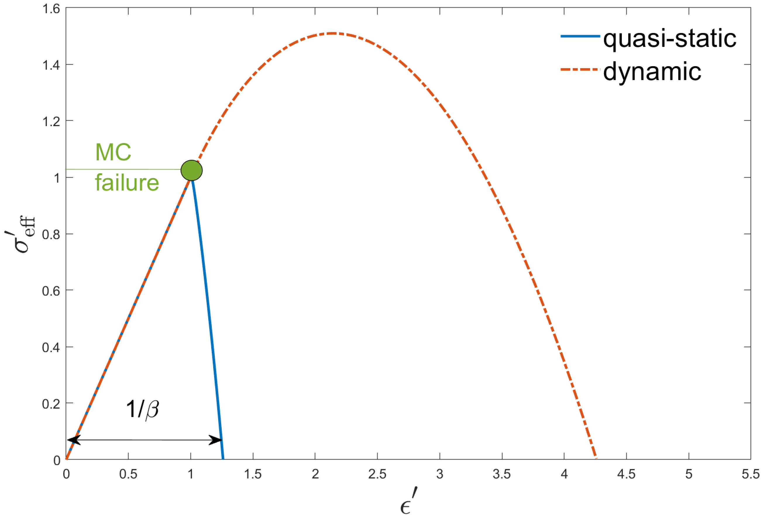
Figure 4 compares strain stress responses for three different model and loading scenarios. The loading considered can correspond to any of the strengths in (4). The nondimensional scalar elastic stress, strain, and effective stress are defined as , , and , respectively, where , , and are the scalar elastic stress, strain, and effective stress. (Note that the scalar elastic stress measure in this section is different from the normal stress component in the Mohr-Coulomb criterion; cf. Figure 1.) These scalar values, , and stiffness C correspond to a particular loading condition; for example for uniaxial tensile loading , , , (cf. (4b)). The corresponding stiffness is and , for plane stress and plane strain conditions, respectively, where E and are the elastic modulus and Poisson ratio.
As loading () increases, the scalar stress c increases until in Figure 2 for the given loading condition. This corresponds to . For the MC model, material is deemed to fail instantaneously, for . This sudden failure is shown by the green circle in the figure. The damage model regularizes the MC failure criterion. For the quasi-static loading , thus throughout the loading. Given the linear dependence of on c in (5), linearly decreases from unity to zero as increases from unity to . As, the response of the damage model tends to that of the un-regularized MC model, clarifying why is called the brittleness factor. Regardless of the rate of loading for , remains bounded by ; cf. (6). This results in a delayed damage response where D falls far behind its quasi-static limit for higher rates of loading for . This, in turn, increases the maximum effective stress, , failure strain, , and toughness, i.e., the area under the strain-stress curve. That is, the time-delay evolution law (6) can qualitatively model material’s well-known stress rate effect. The dynamic solution in Figure 4 corresponds to a nondimensional strain rate of 3. For lower and higher nondimensional loading rates, the stress response gets closer to the quasi-static response and further expands, respectively.
If the quasi-static damage model where to be used, it would suffer the mesh-sensitivity problem of the early damage models. The introduction of an intrinsic length scale addresses this issue. The length scale is either used in conjunction of added higher spatial order derivative terms in a local damage model [21,22] or by nonlocal integration of certain fields, e.g., strain, over neighborhoods of size . However, both approaches are computationally expensive. The proposed damage model is much easier to implement, since it is simply an ODE in time. It also maintains the hyperbolicity of the elastodynamic problem which is critical for the solution of the coupled problem by the aSDG problem. Finally, the interaction of elastic wave speeds with the intrinsic time scale indirectly introduces a length scale for the damage problem. While this length scale is not relevant for very low rate loading problems [52], at moderate to high loading rates it is expected to resolve the mesh sensitivity problem of local damage models.
2.4. aSDG Method
The asynchronous Spacetime Discontinuous Galerkin (aSDG) method, formulated for elastodynamic problem in [32], is use for dynamic fracture analysis. The Tent Pitching algorithm [53] is used to advance the solution in time by continuous erection of patches of elements whose exterior patch boundaries satisfy a special causality constraint. This results in a local and asynchronous solution process. In addition, since spacetime is directly discretized by finite elements, the order of accuracy can be arbitrarily high both in space and time directions. This is in contrast to conventional finite element plus time marching algorithms where increasing the order of accuracy in time is not straightforward.
In addition to the displacement field for the elastodynamic problem, the damage field D is discretized in spacetime. The finite elements solve the weak form of elastodynamic balance laws, cf. Section 2.2, and the damage evolution Equation (6), . Since the damage evolution is simply an ODE and maintains the hyperbolicity of the problem, the solution of the coupled elastodynamic-damage problem lends itself to the aSDG method. In addition, the satisfaction of balance laws per element for discontinuous Galerkin methods results in a very accurate discrete solution of the damage evolution equation. We refer the reader to [31] for more details on the aSDG implementation of the problem, including the specification of jump conditions, and initial/boundary conditions for the damage evolution equation.
2.5. Realization of Stochastic Damage Model Parameters
As discussed in Section 1, incorporating material inhomogeneity is quite important to capture realistic failure response of quasi-brittle materials. The inhomogeneity is both in elastic and fracture properties. If an isotropic material model is assumed at the mesoscale, often only the elastic modulus is deemed to be a random field as in [54]. However, in general the entire elasticity tensor should be considered as a tensorial random field. However, often due to the higher effect that fracture properties have on macroscopic failure response, only they are considered to be random and inhomogeneous.
For a general fracture model, strength, energy, and initial damage state are the main model parameters. For the MC model, the friction angle (or friction coefficient k) and cohesion are the model parameters used to determine c and from (2) and (5), respectively. Cohesion is the parameter that is associated with fracture strength. The relaxation time in (6) and brittleness factor determine the area under the strain-stress curve for different loading rates in Figure 4. That is, they determine the fracture energy of the damage model. Finally, the initial condition for damage parameter, , corresponds to the initial state of material. In the present work, among strength, energy, and initial damage parameters, we consider inhomogeneity only in the strength property. This is in accord with a majority of similar studies in the literature such as [55,56,57,58,59,60].
Accordingly, the only random field in the present study is cohesion . For a macroscopically homogeneous material, the point-wise and two-point statistics of the random field are spatially uniform. For the point-wise statistics, the mean and standard deviation of the random field are the main parameters. For the two-point statistics the form of the correlation function and the correlation length, i.e., the length scale at which the field spatially varies are the main parameters. In [54], where the elastic modulus is considered to a random field, standard deviation and correlation length of the random field are considered as the main parameters that impact fracture response. The realization of random fields for fracture strength and the subsequent fracture analysis becomes more expensive as the correlation length tends to zero. In [54] it is shown that certain macroscopic fracture statistics converge as the correlation length tends to zero. That is, by maintaining sufficient level of material inhomogeneity through using a small enough correlation length, accurate representation of macroscopic fracture response can be obtained.
We treat cohesion as a stationary random field with certain standard deviation and correlation length . The statistics of this random field can be systematically obtained by using Statistical Volume Elements (SVEs), as shown in [60,61]. However, for simplicity and better control on the effect of these parameters, we artificially manufacture random fields with certain and . The distribution of is assumed to follow a probability structure where and are the mean and standard deviation of the normal field. The corresponding mean and standard deviation of the log normal field for are and .
Once the underlying correlation function form and length, and point-wise Probability Distribution Function (PDF) are specified, there are a number of statistical methods to realize consistent random fields. We use the Karhunen-Loéve (KL) method [62,63] to realize a random field by an expansion of its covariance kernel; the field is described by the series,
where the denumerable set of eigenvalues and eigenfunctions are obtained as solutions of the Fredholm equation, i.e., the generalized eigenvalue problem (EVP), as detailed [64]. Since the eigenvalues monotonically decrease, the truncated series with an appropriate value of the upper limit n instead of ∞ in (10), can precisely represent the statics of the underlying random field. For practical use of the KL method, random variables should be statistically unrelated. This condition is automatically satisfied for Gaussian fields. Thus, we sample Gaussian random fields with the mean and standard deviation . To obtain the final random field for , we need to take the exponent of the realized Gaussian random field. There are some technical challenges for using two distinct grids for the aSDG finite element solution in spacetime and the realized random field for in a material grid. For more discussion on the use of KL method for fracture analysis and aSDG analysis of domains with random properties, we refer the reader to [65].
3. Numerical Results
We consider rock failure under dynamic compressive loading, and study the effect of mesh size, load amplitude, and material inhomogeneity on damage pattern. The geometry and loading description are shown in Figure 5, where a rectangular domain of width and height is subject to compressive loading on top and bottom faces. The traction ramps up from zero to the sustained value of in ramp time . Zero tangential traction is applied on these faces to model a frictionless loading interface. A traction free boundary condition is applied on the vertical sides of the domain. We assume a 2D plain-strain condition with material properties reported in Table 1.
For this 2D problem, the spacetime mesh corresponds to a grid of tetrahedron elements. The solution is advanced to the final time by an asynchronous patch-by-patch solution algorithm. The time increment of a pitched vertex is calculated based on the wave speed, spatial geometry, and sizes of elements around; cf. Section 2.4 and [32,53] for more details. We use third order polynomial basis functions for damage and displacement fields in space and time.
As shown in Figure 6, we use three different structured grids of , , and squares, where each square is divided into two triangles. These are labeled as coarse, medium, and fine meshes, respectively. One of the numerical challenges in damage mechanics that affects the convergence of the Newton-Raphson method is the zero stiffness issue when damage is equal to unity. One way to avoid this problem is multiplying the damage value used in (8) by a positive reduction factor less than unity. Herein, we select a reduction factor of .
3.1. Homogeneous Material
3.1.1. Mesh Sensitivity
The dependence of damage response on the resolution of the underlying discrete grid is a well-known problem for non-regularized continuum damage models. As described in Section 2.3.2, the proposed time-delay damage model introduces an inherent length scale proportional to the relaxation time and longitudinal elastic wave speed, i.e., . To show mesh-objectivity of the results, we compare the damage evolution for coarse and medium meshes in Figure 7. For this numerical example, material properties are homogeneous and listed in Table 1, and the loading magnitude is .
Figure 7 shows an excellent agreement between the solutions of the two meshes at early and evolved stages of damage evolution. We also refer the reader to [31] for a more detailed study of mesh objectivity for a tensile fracture problem where damage localization zone converges to a region of finite width. We reiterate that the time-delay formulation addresses the mesh-objectivity problem with much less computational difficulty than the non-local integration-based and gradient-based damage models. Moreover, it does not violate the hyperbolicity of the problem. This facilitates the use of the aSDG method and is consistent with the physical observation that damage propagates with a finite speed [66].
3.1.2. The Effect of Load Amplitude
In the previous example, the stress level was sufficiently high to initiate damage near the loading edges, from the early stages of the solution. The stress state in the middle of top and bottom faces is approximately similar to bi-axial compressive condition; material tends to expand in the horizontal direction because of the Poisson effect while the surrounding material prevents its deformation. However, the stress state around the corners is close to an unconfined uni-axial compressive condition because of the stress-free conditions at left and right boundaries. The higher differences between compressive stresses in the Mohr circle results in a higher value for c; cf. (2). Thus according to the MC failure criterion, the corner zones are more susceptible to an earlier time for damage initiation and higher damage values. This is verified by the higher damage values around the corners in Figure 7a,b. After the initiation of damage at corners, damage diffuses towards the middle of the domain.
To study the effect of load amplitude, we reduce the peak stress such that damage initiates in the middle of the domain. The vertical normal stress magnitude roughly doubles across the entire width when the stress waves collide in the middle of the domain. The load for this problem is chosen such that it is not large enough to initiate damage when the stress wave enters from the top and bottom edges, but is sufficient to cause damage in the middle of domain due to the doubling effect. We call this condition the low amplitude case, corresponding to , and refer to the previous peak stress problem as the high amplitude case. As shown in Figure 8a, the initial damage occurs when the peak stress reaches the middle of the domain; i.e., at which is well predicted by the numerical result. After the collision, the magnified reflected waves are sufficiently high to overcome the cohesion of rock. Thereafter, damage diffuses toward boundaries where the waves are propagating to; see Figure 8b–d. This failure mechanism is completely different from that of the high amplitude case where the damage initiates in a shear dominated regime at the corners. Therefore, load amplitude has a significant impact on damage pattern and failure mechanism. For a better comparison, we provide the damage response at various times for the high amplitude case in Figure 9.
3.2. Heterogeneous Material
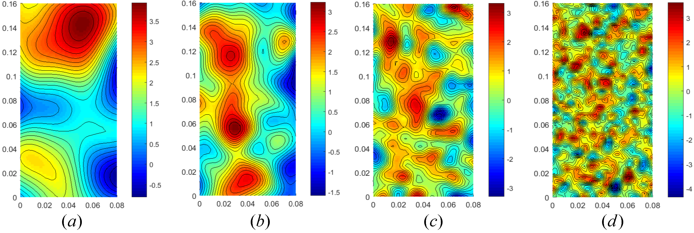
As detailed in Section 2.5, for the analysis of inhomogeneous rock masses, we assume that cohesion is a random field. This analysis expands our preliminary comparison of the response of homogeneous and heterogeneous rock in [67]. We construct four random fields using the KL method with the mean cohesion value of , similar to the spatially uniform used in the preceding examples for homogeneous rock. The standard deviation is set to . The correlation lengths of , , , and are used, where for each correlation length one random field realization is generated by the KL method. These random fields are shown in Figure 10. A smaller correlation length indicates faster variations in cohesion from one spatial point to another, so it corresponds to a more locally heterogeneous field. These random fields are constructed with the first 2000 terms of the KL series. For the following results, we use the fine mesh to have an adequate resolution for capturing the underlying inhomogeneity.
3.2.1. Low Amplitude Load
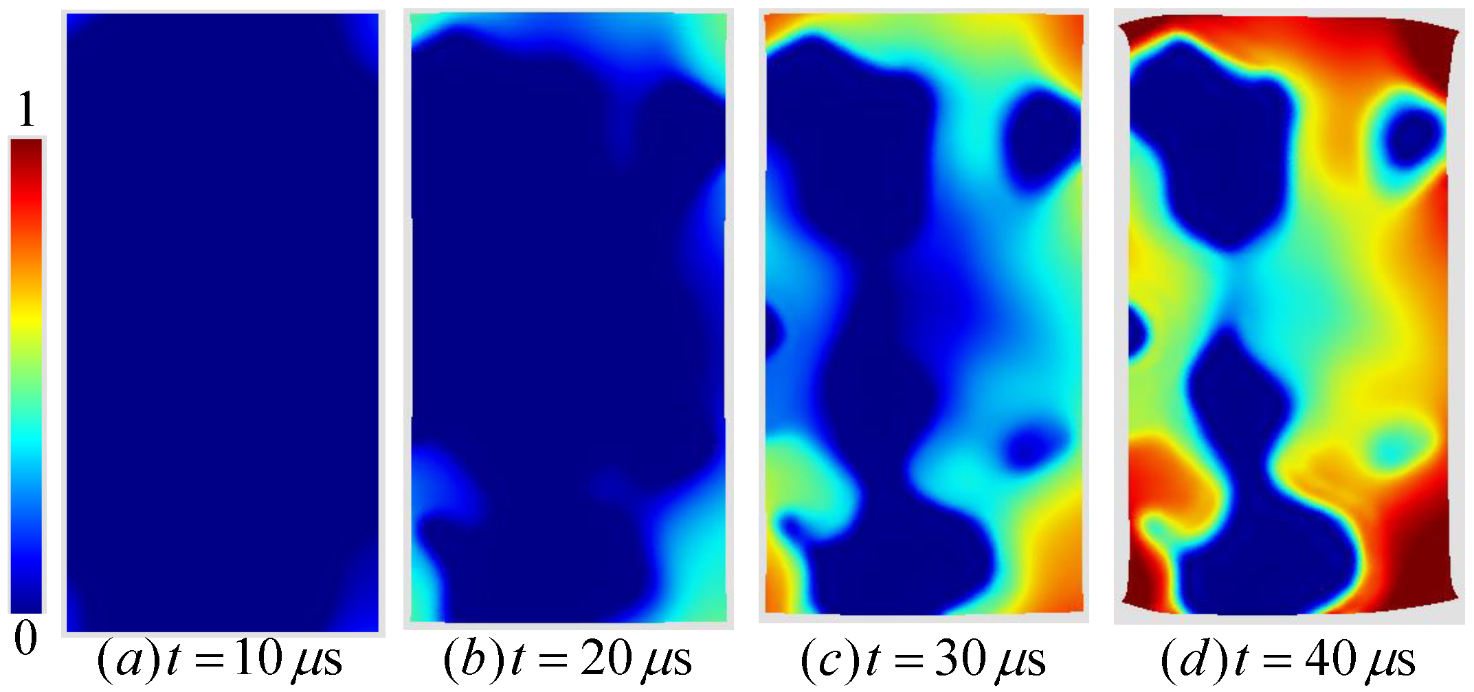
In this section, we study the effect of heterogeneity on damage response for the low amplitude condition. Figure 11 shows the damage response for at various times. From the cohesion map in Figure 10a, we observe that varies very slowly in space. It takes the highest values near the top boundary and the lowest ones at three spots close to the left and right boundaries; weak zones are colored by blue. In Figure 8a, the initial damage zone begins when the stress waves collide in the middle of the domain. The particular form of this realization for actually favors damage accumulation in the center, given that a higher strength zone is near the top boundary in Figure 10a. As shown in Figure 11, damage initiates and accumulates both in this center location and in the three aforementioned weak sites close to the boundaries. Thus, the form of the failure pattern follows both the weak points in the material and locations with higher stress values in general. By comparison of Figure 8 and Figure 11, we also observe that the earlier initiation of damage in weaker sites results in a response with more concentrated damage zones. Finally, the damage initiation time is almost the same as that for the homogeneous rock, and in both cases it is right after the collision of the waves at .
Figure 12, Figure 13 and Figure 14 show the damage evolution for heterogeneous cohesion fields with correlation lengths equal to , , and , respectively. According to Figure 12a, Figure 13a and Figure 14a, the time for damage initiation decreases as the correlation length gets smaller, i.e., when the heterogeneity is increasing.
It is well accepted in the literature that one of the main reasons for localization and softening behavior in brittle materials is their heterogeneous structure at microscale [68,69,70]; the weaker points in material begin to fail earlier. This results in an increased stress concentration in the damaging zones and the shielding of the surrounding areas. That is, the inhomogeneity in material properties promotes inhomogeneity and localization in the stress field. Unlike ductile materials, there are not much energy dissipative reserves, for example from plasticity, to balance the stress field. Figure 11d, Figure 12d, Figure 13d and Figure 14d reveal a crucial impact of the correlation length on failure mechanism; this is a transition from diffusive damage propagation to a more localized response as the correlation length gets smaller. This agrees with the preceding discussion on the promotion of damage localization by material inhomogeneity. In fact, for the solutions with the lowest correlation length, even the mode and propagation of failure is significantly different than that of a homogenous material; in Figure 8d and Figure 14d, the effect of the weakest point of the material is high to an extent that damage initiates and accumulates in a more distributed sense, as opposed to the damage accumulation in the central zone in Figure 8.
3.2.2. High Amplitude Load
Figure 15, Figure 16, Figure 17 and Figure 18 show the evolution of the damage field for correlation lengths to . We observe a very good match between damage localization sites and the locations of material weak points in Figure 10b–d. Moreover, as we decrease the correlation length, the time of damage initiation decreases; cf. Figure 15a, Figure 16a, Figure 17a and Figure 18a.
From the final damage pattern in Figure 9d for the homogeneous domain, one observes that for high amplitude loading extensive damage is experienced almost everywhere, especially close to the top and bottom boundaries. There is little resemblance between this solution and those for high correlation random fields in Figure 15d and Figure 16d. Similarly for the low amplitude load, high differences are observed between the solutions of homogeneous, Figure 8d, and inhomogeneous domains with high correlation lengths, Figure 11d and Figure 12d. This is due to the fact that for such large correlation lengths, the large islands of low strength greatly impact the response.
In contrast, as the correlation length decreases, the overall material properties are almost the same in all areas, except the inhomogeneities that are observed at smaller length scales. Consequently, in comparison of damage patterns for the homogeneous rock in Figure 9d and rocks with small correlation length for in Figure 17d and Figure 18d, a very similar overall response is observed; in all cases, damage is widespread in the domain, with the top and bottom sides experiencing the highest damage. In contrast, there is no resemblance between the damage patterns of homogeneous domain in Figure 8d and those for low correlation length fields in Figure 13d and Figure 14d. The reason is that for this low amplitude of load, damage can only accumulate in the center of the homogeneous domain, whereas for inhomogeneous domains damage can accumulate from weak points outside of this zone; this greatly affect the final damage pattern.
The statistical continuum damage model enhances the accuracy of conventional continuum damage models, and its solutions are more consistent with sharp interface fracture models. The reason are as follows. First, damage initiation zones from material weak points are more concentrated and better resemble crack nucleation events. Second, damaged zones tend to propagate in crack-like features with specific inclined directions rather than the diffuse response around the initiation points. For example, in Figure 18d, many localized zones resemble cracks at 45 degree and steeper relative to the vertical direction. This features qualitatively match other numerical and experimental observations [71,72,73,74,75]. Specifically, based on the MC failure criterion, cracks are formed at angles with respect to the compressive loading direction. This example demonstrates that a damage model based on uniform material properties not only misses crack-like damage localization features, but can also incorrectly predict the location of zones with the maximum overall damage accumulation (low load example).
3.2.3. Mesh Sensitivity
The mesh sensitivity of diffusive damage response for the sample with homogeneous properties was presented in Section 3.1.1. Here, we study the effect of mesh size for domains with heterogeneous cohesion that result in a localized damage response. Figure 19 compares damage responses for the domain with at . The results are presented for different load amplitudes and mesh sizes. The same results are presented in Figure 20 for the smallest correlation length at . While, there is a good agreement between the results obtained by medium and coarse meshes for both load conditions, the solutions for the largest correlation length in Figure 19 show a better agreement. This is due to the fact that the details of the solution are at the scale of the correlation length; thus, as smaller correlation lengths are used for material properties, finer finite elements should be used to accurately capture the details of the solution.
4. Conclusions
We presented a dynamic bulk damage model, based on the time-delay evolution law in [3]. The relaxation time indirectly introduces an intrinsic length scale for dynamic fracture problems. This resolves the mesh sensitivity problem of early local damage models. Moreover, by limiting the maximum damage rate, the model qualitatively captures stress rate effect, in that, both strength and toughness increase when the loading rate increases. The ODE form of the evolution model greatly simplifies the implementation of the damage model and maintains the hyperbolicity of the elastodynamic problem.
The coupled elastodynamic-damage problem was implemented by the aSDG method to solve a uniaxial compressive fracture problem for rock. The MC model is used to formulate a damage force model. In the process of damage accumulation, the effective stress tends from the initial elastic limit at to its hydrostatic compressive value at . The MC model also captures rock strengthening effect as hydrostatic pressure increases. In contrast, damage models that are based on spectral positive and negative decomposition of strain (or stress) tensor, fail to model failure under compressive response.
To model the effect of material inhomogeneity, cohesion was assumed to be a random field. Two different macroscopic compressive load amplitudes were used for this study. For a homogeneous material, the higher load amplitude initiates damage as the compressive wave enters the domain, whereas for the lower load damage initiates only in the center of the domain where stress doubling effect occurs upon the intersection of compressive waves. Four lognormal fields with different correlation lengths were generated for . It was shown that inhomogeneity could significantly alter the failure response of an otherwise homogeneous rock. For example, for the higher load amplitude, unlike the homogeneous case, damage initiates in the center of the domain. This is due to the particular form of the realized random field where a large zone of low is sampled in the center of the domain. Moreover, for the lower load amplitude damage can initiate everywhere in the domain as the waves travel toward the center of the domain. This is due to the weaker sampled at these locations, which does not require the stress wave doubling effect to initiate damage. Moreover, even the zones that eventually accumulate the highest damage can be significantly different between models with homogeneous and inhomogeneous properties, even as the correlation length tends to zero (low load amplitude example).
Another problem of using a homogeneous material model is the inability or difficulty of bulk damage models to capture sharp localization zones. In contrast, as lower correlation lengths were used for inhomogeneous domains, the fracture pattern became more realistic and resembled the results that are obtained by more accurate sharp interface models [43]. In particular, the MC model predicts fractures at degree angles with respect to the compressive load direction. For the lowest correlation lengths, localized damage zones with angles roughly in the range to are observed. These features are better resolved with the higher resolution finite element mesh, confirming that finer meshes are required for the solution of problems with more rapid variation of material properties.
There are several extensions to the present work. First, the form of effective stress (8) implies that friction coefficient is zero at complete damage (), whereas jointed (damaged) rock may still possess some residual friction coefficient. This will enhance the angle of localized regions in Figure 18d. Second, MC criterion is not appropriate for rock tensile fracture analysis and the damage force can be formulated by Hoek-Brown [76] and other more accurate models. Third, as shown in [77], rock anisotropy, for example induced by the existence of bedding planes, can affect fracture angle under compressive loading. Anisotropic failure criteria such as those in [78,79] can be used to formulate the damage force. Finally, mesh adaptive operations in spacetime [33] can drastically reduce the computational cost of the formulated aSDG method for this bulk damage model.
Author Contributions
B.B., R.A., and P.L.C. were responsible for the conceptualization, methodology, software development. P.L.C. was responsible for the random domain creation. B.B. was responsible for the formulation/implementation of the bulk damage model and dynamic fracture simulation/visualization. R.A. was responsible for aSDG software development writing review and editing, supervision, and project administration. The manuscript was written by R.A. and B.B.
Funding
The authors gratefully acknowledge partial support for this work via the U.S. National Science Foundation (NSF), CMMI—Mechanics of Materials and Structures (MoMS) program grant number 1538332 and NSF, CCF—Scalable Parallelism in the Extreme (SPX) program grant number 1725555.
Conflicts of Interest
The authors declare no conflict of interest.
Abbreviations
The following abbreviations are used in this manuscript:
| MDPI | Multidisciplinary Digital Publishing Institute |
| DOAJ | Directory of open access journals |
| KL | Karhunen-Loève |
| aSDG | asynchronous Spacetime Discontinuous Galerkin Method |
References
- Dugdale, D.S. Yielding of steel sheets containing slits. J. Mech. Phys. Solids 1960, 8, 100–104. [Google Scholar] [CrossRef]
- Barenblatt, G.I. The mathematical theory of equilibrium of cracks in brittle fracture. Adv. Appl. Mech. 1962, 7, 55–129. [Google Scholar]
- Allix, O.; Feissel, P.; Thévenet, P. A delay damage mesomodel of laminates under dynamic loading: Basic aspects and identification issues. Comput. Struct. 2003, 81, 1177–1191. [Google Scholar] [CrossRef]
- Alfano, G. On the influence of the shape of the interface law on the application of cohesive-zone models. Compos. Sci. Technol. 2006, 66, 723–730. [Google Scholar] [CrossRef]
- Parrinello, F.; Failla, B.; Borino, G. Cohesive-frictional interface constitutive model. Int. J. Solids Struct. 2009, 46, 2680–2692. [Google Scholar] [CrossRef]
- Nguyen, V.P. Discontinuous Galerkin/extrinsic cohesive zone modeling: Implementation caveats and applications in computational fracture mechanics. Eng. Fract. Mech. 2014, 128, 37–68. [Google Scholar] [CrossRef]
- Abedi, R.; Haber, R.B. Spacetime simulation of dynamic fracture with crack closure and frictional sliding. Adv. Model. Simul. Eng. Sci. 2018, 5, 22. [Google Scholar] [CrossRef]
- Spring, D.W.; Leon, S.E.; Paulino, G.H. Unstructured polygonal meshes with adaptive refinement for the numerical simulation of dynamic cohesive fracture. Int. J. Fract. 2014, 189, 33–57. [Google Scholar] [CrossRef]
- Rangarajan, R.; Lew, A.J. Universal meshes: A method for triangulating planar curved domains immersed in nonconforming meshes. Int. J. Numer. Methods Eng. 2014, 98, 236–264. [Google Scholar] [CrossRef]
- Abedi, R.; Omidi, O.; Enayatpour, S. A mesh adaptive method for dynamic well stimulation. Comput. Geotech. 2018, 102, 12–27. [Google Scholar] [CrossRef]
- Belytschko, T.; Black, T. Elastic crack growth in finite elements with minimal remeshing. Int. J. Numer. Methods Eng. 1999, 45, 601–620. [Google Scholar] [CrossRef]
- Moes, N.; Dolbow, J.; Belytschko, T. A finite element method for crack growth without remeshing. Int. J. Numer. Methods Eng. 1999, 46, 131–150. [Google Scholar] [CrossRef]
- Khoei, A.; Vahab, M.; Hirmand, M. An enriched–FEM technique for numerical simulation of interacting discontinuities in naturally fractured porous media. Comput. Methods Appl. Mech. Eng. 2018, 331, 197–231. [Google Scholar] [CrossRef]
- Duarte, C.A.; Babuška, I.; Oden, J.T. Generalized finite element methods for three-dimensional structural mechanics problems. Comput. Struct. 2000, 77, 215–232. [Google Scholar] [CrossRef]
- Strouboulis, T.; Babuška, I.; Copps, K. The design and analysis of the Generalized Finite Element Method. Comput. Methods Appl. Mech. Eng. 2000, 181, 43–69. [Google Scholar] [CrossRef]
- Silling, S.A.; Lehoucq, R. Peridynamic theory of solid mechanics. In Advances in Applied Mechanics; Elsevier: Amsterdam, The Netherlands, 2010; Volume 44, pp. 73–168. [Google Scholar]
- Ha, Y.D.; Bobaru, F. Studies of dynamic crack propagation and crack branching with peridynamics. Int. J. Fract. 2010, 162, 229–244. [Google Scholar] [CrossRef] [Green Version]
- Rabczuk, T.; Ren, H. A peridynamics formulation for quasi-static fracture and contact in rock. Eng. Geol. 2017, 225, 42–48. [Google Scholar] [CrossRef]
- Lasry, D.; Belytschko, T. Localization limiters in transient problems. Int. J. Solids Struct. 1988, 24, 581–597. [Google Scholar] [CrossRef]
- Loret, B.; Prevost, J.H. Dynamic strain localization in elasto-(visco-) plastic solids, Part 1. General formulation and one-dimensional examples. Comput. Methods Appl. Mech. Eng. 1990, 83, 247–273. [Google Scholar] [CrossRef]
- Peerlings, R.; De Borst, R.; Brekelmans, W.; Geers, M. Gradient-enhanced damage modelling of concrete fracture. Mech. Cohes.-Frict. Mater. 1998, 3, 323–342. [Google Scholar] [CrossRef]
- Comi, C. Computational modelling of gradient-enhanced damage in quasi-brittle materials. Mech. Cohes.-Frict. Mater. 1999, 4, 17–36. [Google Scholar] [CrossRef]
- Peerlings, R.; Geers, M.; De Borst, R.; Brekelmans, W. A critical comparison of nonlocal and gradient-enhanced softening continua. Int. J. Solids Struct. 2001, 38, 7723–7746. [Google Scholar] [CrossRef]
- Pereira, L.; Weerheijm, J.; Sluys, L. A new effective rate dependent damage model for dynamic tensile failure of concrete. Eng. Fract. Mech. 2017, 176, 281–299. [Google Scholar] [CrossRef]
- Allix, O.; Deü, J.F. Delayed-damage modelling for fracture prediction of laminated composites under dynamic loading. Eng. Trans. 1997, 45, 29–46. [Google Scholar]
- Lyakhovsky, V.; Hamiel, Y.; Ben-Zion, Y. A non-local visco-elastic damage model and dynamic fracturing. J. Mech. Phys. Solids 2011, 59, 1752–1776. [Google Scholar] [CrossRef]
- Häussler-Combe, U.; Panteki, E. Modeling of concrete spallation with damaged viscoelasticity and retarded damage. Int. J. Solids Struct. 2016, 90, 153–166. [Google Scholar] [CrossRef]
- Junker, P.; Schwarz, S.; Makowski, J.; Hackl, K. A relaxation-based approach to damage modeling. Contin. Mech. Thermodyn. 2017, 29, 291–310. [Google Scholar] [CrossRef]
- de Borst, R.; Verhoosel, C.V. Gradient damage vs phase-field approaches for fracture: Similarities and differences. Comput. Methods Appl. Mech. Eng. 2016, 312, 78–94. [Google Scholar] [CrossRef] [Green Version]
- Mandal, T.K.; Nguyen, V.P.; Heidarpour, A. Phase field and gradient enhanced damage models for quasi-brittle failure: A numerical comparative study. Eng. Fract. Mech. 2019, 207, 48–67. [Google Scholar] [CrossRef]
- Bahmani, B.; Abedi, R. Asynchronous Spacetime Discontinuous Galerkin Formulation for a Hyperbolic Time-Delay Bulk Damage Model. J. Eng. Mech. 2019. accepted. [Google Scholar]
- Abedi, R.; Haber, R.B.; Petracovici, B. A spacetime discontinuous Galerkin method for elastodynamics with element-level balance of linear momentum. Comput. Methods Appl. Mech. Eng. 2006, 195, 3247–3273. [Google Scholar] [CrossRef]
- Abedi, R.; Haber, R.B.; Thite, S.; Erickson, J. An h–adaptive spacetime–discontinuous Galerkin method for linearized elastodynamics. Revue Européenne de Mécanique Numérique (Eur. J. Comput. Mech.) 2006, 15, 619–642. [Google Scholar]
- Bischoff, P.H.; Perry, S.H. Impact behavior of plain concrete loaded in uniaxial compression. J. Eng. Mech. 1995, 121, 685–693. [Google Scholar] [CrossRef]
- Al-Ostaz, A.; Jasiuk, I. Crack initiation and propagation in materials with randomly distributed holes. Eng. Fract. Mech. 1997, 58, 395–420. [Google Scholar] [CrossRef]
- Kozicki, J.; Tejchman, J. Effect of aggregate structure on fracture process in concrete using 2D lattice model. Arch. Mech. 2007, 59, 365–384. [Google Scholar]
- Bazant, Z.; Novak, D. Probabilistic nonlocal theory for quasibrittle fracture initiation and size effect—I: Theory. J. Eng. Mech. 2000, 126, 166–174. [Google Scholar] [CrossRef]
- Rinaldi, A.; Krajcinovic, D.; Mastilovic, S. Statistical damage mechanics and extreme value theory. Int. J. Damage Mech. (USA) 2007, 16, 57–76. [Google Scholar] [CrossRef]
- Bazant, Z.P.; Le, J.L. Probabilistic Mechanics of Quasibrittle Structures: Strength, Lifetime, and Size Effect; Cambridge University Press: Cambridge, UK, 2017. [Google Scholar]
- Weibull, W. A statistical theory of the strength of materials. R. Swed. Inst. Eng. Res. 1939, 151, 1–45. [Google Scholar]
- Weibull, W. A statistical distribution function of wide applicability. J. Appl. Mech. 1951, 18, 293–297. [Google Scholar]
- Abedi, R.; Omidi, O.; Clarke, P. Numerical simulation of rock dynamic fracturing and failure including microscale material randomness. In In Proceedings of the 50th US Rock Mechanics/Geomechanics Symposium, Houston, TX, USA, 26–29 June 2016. ARMA 16-0531. [Google Scholar]
- Abedi, R.; Haber, R.; Elbanna, A. Mixed-mode dynamic crack propagation in rocks with contact-separation mode transitions. In In Proceedings of the 51th US Rock Mechanics/Geomechanics Symposium, San Francisco, CA, USA, 25–28 June 2017. ARMA 17-0679. [Google Scholar]
- Abedi, R.; Haber, R.B.; Clarke, P.L. Effect of random defects on dynamic fracture in quasi-brittle materials. Int. J. Fract. 2017, 208, 241–268. [Google Scholar] [CrossRef]
- Clarke, P.; Abedi, R.; Bahmani, B.; Acton, K.; Baxter, S. Effect of the spatial inhomogeneity of fracture strength on fracture pattern for quasi-brittle materials. In In Proceedings of the ASME 2017 International Mechanical Engineering Congress & Exposition, IMECE 2017, Tampa, FL, USA, 3–9 November 2017; p. V009T12A045. [Google Scholar]
- Hoek, E.; Brown, T. Underground Excavations in Rock; Geotechnics and Foundations; Taylor & Francis: Stroud, UK, 1980. [Google Scholar]
- Suffis, A.; Lubrecht, T.A.; Combescure, A. Damage model with delay effect: Analytical and numerical studies of the evolution of the characteristic damage length. Int. J. Solids Struct. 2003, 40, 3463–3476. [Google Scholar] [CrossRef]
- Murakami, S. Continuum Damage Mechanics; Springer: New York, NY, USA, 2012. [Google Scholar]
- Mazars, J. Application de la Mécanique de l’Endommagement au Comportement non Linéaire et à la Rupture du Béton de Structure. Ph.D. Thesis, Universite Pierre et Marie Curie, Paris, France, 1984. [Google Scholar]
- Jirásek, M.; Patzák, B. Consistent tangent stiffness for nonlocal damage models. Comput. Struct. 2002, 80, 1279–1293. [Google Scholar] [CrossRef]
- Moreau, K.; Moës, N.; Picart, D.; Stainier, L. Explicit dynamics with a non-local damage model using the thick level set approach. Int. J. Numer. Methods Eng. 2015, 102, 808–838. [Google Scholar] [CrossRef]
- Londono, J.G.; Berger-Vergiat, L.; Waisman, H. An equivalent stress-gradient regularization model for coupled damage-viscoelasticity. Comput. Methods Appl. Mech. Eng. 2017, 322, 137–166. [Google Scholar] [CrossRef]
- Abedi, R.; Chung, S.H.; Erickson, J.; Fan, Y.; Garland, M.; Guoy, D.; Haber, R.; Sullivan, J.M.; Thite, S.; Zhou, Y. Spacetime meshing with adaptive refinement and coarsening. In Proceedings of the Twentieth Annual Symposium on Computational Geometry, SCG ’04, Brooklyn, NY, USA, 8–11 June 2004; ACM: New York, NY, USA, 2004; pp. 300–309. [Google Scholar] [Green Version]
- Dimas, L.; Giesa, T.; Buehler, M. Coupled continuum and discrete analysis of random heterogeneous materials: Elasticity and fracture. J. Mech. Phys. Solids 2014, 63, 481–490. [Google Scholar] [CrossRef]
- Carmeliet, J.; Hens, H. Probabilistic nonlocal damage model for continua with random field properties. J. Eng. Mech. 1994, 120, 2013–2027. [Google Scholar] [CrossRef]
- Zhou, F.; Molinari, J. Stochastic fracture of ceramics under dynamic tensile loading. Int. J. Solids Struct. 2004, 41, 6573–6596. [Google Scholar] [CrossRef]
- Schicker, J.; Pfuff, M. Statistical Modeling of fracture in quasi-brittle materials. Adv. Eng. Mater. 2006, 8, 406–410. [Google Scholar] [CrossRef]
- Levy, S.; Molinari, J. Dynamic fragmentation of ceramics, signature of defects and scaling of fragment sizes. J. Mech. Phys. Solids 2010, 58, 12–26. [Google Scholar] [CrossRef] [Green Version]
- Daphalapurkar, N.; Ramesh, K.; Graham-Brady, L.; Molinari, J. Predicting variability in the dynamic failure strength of brittle materials considering pre-existing flaws. J. Mech. Phys. Solids 2011, 59, 297–319. [Google Scholar] [CrossRef]
- Acton, K.A.; Baxter, S.C.; Bahmani, B.; Clarke, P.L.; Abedi, R. Voronoi tessellation based statistical volume element characterization for use in fracture modeling. Comput. Methods Appl. Mech. Eng. 2018, 336, 135–155. [Google Scholar] [CrossRef]
- Bahmani, B.; Yang, M.; Nagarajan, A.; Clarke, P.L.; Soghrati, S.; Abedi, R. Automated homogenization-based fracture analysis: Effects of SVE size and boundary condition. Comput. Methods Appl. Mech. Eng. 2019, 345, 701–727. [Google Scholar] [CrossRef]
- Karhunen, K.; Selin, I. On Linear Methods in Probability Theory; Rand Corporation: Santa Monica, CA, USA, 1960. [Google Scholar]
- Loéve, M. Probability Theory; Springer: New York, NY, USA, 1977. [Google Scholar]
- Ghanem, R.; Spanos, P. Stochastic Finite Elements: A Spectral Approach; Springer: New York, NY, USA, 1991. [Google Scholar]
- Clarke, P.; Abedi, R. Fracture modeling of rocks based on random field generation and simulation of inhomogeneous domains. In In Proceedings of the 51th US Rock Mechanics/Geomechanics Symposium, San Francisco, CA, USA, 25–28 June 2017. ARMA 17-0643. [Google Scholar]
- Häussler-Combe, U.; Kühn, T. Modeling of strain rate effects for concrete with viscoelasticity and retarded damage. Int. J. Impact Eng. 2012, 50, 17–28. [Google Scholar] [CrossRef]
- Bahmani, B.; Clarke, P.; Abedi, R. A bulk damage model for modeling dynamic fracture in rock. In In Proceedings of the 52th US Rock Mechanics/Geomechanics Symposium, Seattle, Washington, USA, 17–20 June 2018. ARMA 18-826. [Google Scholar]
- Bazant, Z.P.; Belytschko, T.B.; Chang, T.P. Continuum theory for strain-softening. J. Eng. Mech. 1984, 110, 1666–1692. [Google Scholar] [CrossRef]
- Bažant, Z.P.; Belytschko, T.B. Wave propagation in a strain-softening bar: Exact solution. J. Eng. Mech. 1985, 111, 381–389. [Google Scholar] [CrossRef]
- Xu, T.; Yang, S.; Chen, C.; Yang, T.; Zhang, P.; Liu, H. Numerical Investigation of Damage Evolution and Localized Fracturing of Brittle Rock in Compression. J. Perform. Constr. Facil. 2017, 31, 04017065. [Google Scholar] [CrossRef]
- Tang, C.; Tham, L.; Lee, P.; Tsui, Y.; Liu, H. Numerical studies of the influence of microstructure on rock failure in uniaxial compression—Part II: Constraint, slenderness, and size effect. Int. J. Rock Mech. Min. Sci. 2000, 37, 571–583. [Google Scholar] [CrossRef]
- Teng, J.; Zhu, W.; Tang, C. Mesomechanical model for concrete. Part II: Applications. Mag. Concr. Res. 2004, 56, 331–345. [Google Scholar] [CrossRef]
- Li, G.; Tang, C.A. A statistical meso-damage mechanical method for modeling trans-scale progressive failure process of rock. Int. J. Rock Mech. Min. Sci. 2015, 74, 133–150. [Google Scholar] [CrossRef]
- Dinç, Ö.; Scholtès, L. Discrete Analysis of Damage and Shear Banding in Argillaceous Rocks. Rock Mech. Rock Eng. 2018, 51, 1521–1538. [Google Scholar] [CrossRef]
- Rangari, S.; Murali, K.; Deb, A. Effect of Meso-structure on Strength and Size Effect in Concrete under Compression. Eng. Fract. Mech. 2018, 195, 162–185. [Google Scholar] [CrossRef]
- Hoek, E. Strength of jointed rock masses. Geotechnique 1983, 33, 187–223. [Google Scholar] [CrossRef] [Green Version]
- Abedi, R.; Clarke, P.L. Modeling of rock inhomogeneity and anisotropy by explicit and implicit representation of microcracks. In In Proceedings of the 52nd US Rock Mechanics/Geomechanics Symposium, Seattle, WA, USA, 17–20 June 2018. ARMA 18-151-0228-1094. [Google Scholar]
- Pietruszczak, S.; Mroz, Z. On failure criteria for anisotropic cohesive-frictional materials. Int. J. Numer. Anal. Methods Geomech. 2001, 25, 509–524. [Google Scholar] [CrossRef]
- Lee, Y.K.; Pietruszczak, S. Analytical representation of Mohr failure envelope approximating the generalized Hoek-Brown failure criterion. Int. J. Rock Mech. Min. Sci. 2017, 100, 90–99. [Google Scholar] [CrossRef]
Figure 1.
Mohr-Coulomb failure criterion and scalar stress c for a given stress state.

Figure 2.
Relation of different fracture strengths, , , , and to cohesion .

Figure 3.
The effect of brittleness exponent a on the rate of damage evolution.

Figure 4.
Sample quasi-static and dynamic strain versus stress responses.

Figure 5.
Problem description for a rectangle subject to a vertical compressive loading.

Figure 6.
Initial meshes used for the simulations: (a) Coarse, (b) Medium, and (c) Fine.

Figure 7.
Damage responses at different times for two different meshes. Figures (a,b) correspond to the coarse mesh and figures (c,d) correspond to the medium mesh. The results are shown on the deformed mesh with a magnification factor of 300.
Figure 7.
Damage responses at different times for two different meshes. Figures (a,b) correspond to the coarse mesh and figures (c,d) correspond to the medium mesh. The results are shown on the deformed mesh with a magnification factor of 300.

Figure 8.
Damage evolution for the medium mesh and low amplitude load at times: (a) , (b) , (c) , and (d) . The results are shown on the deformed meshes with a magnification factor of 1000.
Figure 8.
Damage evolution for the medium mesh and low amplitude load at times: (a) , (b) , (c) , and (d) . The results are shown on the deformed meshes with a magnification factor of 1000.

Figure 9.
Damage evolution for the medium mesh and high amplitude load at times: (a) , (b) , (c) , and (d) . The results are shown on the deformed meshes with a magnification factor of 300.
Figure 9.
Damage evolution for the medium mesh and high amplitude load at times: (a) , (b) , (c) , and (d) . The results are shown on the deformed meshes with a magnification factor of 300.

Figure 10.
Random field realizations for cohesion with different correlation lengths, , equal to: (a) , (b) , (c) , and (d) .
Figure 10.
Random field realizations for cohesion with different correlation lengths, , equal to: (a) , (b) , (c) , and (d) .

Figure 11.
The evolution of damage field for the low amplitude load and cohesion realization with at times: (a) , (b) , (c) , and (d) .
Figure 11.
The evolution of damage field for the low amplitude load and cohesion realization with at times: (a) , (b) , (c) , and (d) .

Figure 12.
The evolution of damage field for the low amplitude load and cohesion realization with at times: (a) , (b) , (c) , and (d) .
Figure 12.
The evolution of damage field for the low amplitude load and cohesion realization with at times: (a) , (b) , (c) , and (d) .

Figure 13.
The evolution of damage field for the low amplitude load and cohesion realization with at times: (a) , (b) , (c) , and (d) .
Figure 13.
The evolution of damage field for the low amplitude load and cohesion realization with at times: (a) , (b) , (c) , and (d) .

Figure 14.
The evolution of damage field for the low amplitude load and cohesion realization with at times: (a) , (b) , (c) , and (d) .
Figure 14.
The evolution of damage field for the low amplitude load and cohesion realization with at times: (a) , (b) , (c) , and (d) .

Figure 15.
The evolution of damage field for the high amplitude load and cohesion realization with at times: (a) , (b) , (c) , and (d) . The results are shown on the deformed mesh with a magnification factor of 100.
Figure 15.
The evolution of damage field for the high amplitude load and cohesion realization with at times: (a) , (b) , (c) , and (d) . The results are shown on the deformed mesh with a magnification factor of 100.

Figure 16.
The evolution of damage field for the high amplitude load and cohesion realization with at times: (a) , (b) , (c) , and (d) . The results are shown on the deformed mesh with a magnification factor of 100.
Figure 16.
The evolution of damage field for the high amplitude load and cohesion realization with at times: (a) , (b) , (c) , and (d) . The results are shown on the deformed mesh with a magnification factor of 100.

Figure 17.
The evolution of damage field for the high amplitude load and cohesion realization with at times: (a) , (b) , (c) , and (d) . The results are shown on the deformed mesh with a magnification factor of 100.
Figure 17.
The evolution of damage field for the high amplitude load and cohesion realization with at times: (a) , (b) , (c) , and (d) . The results are shown on the deformed mesh with a magnification factor of 100.

Figure 18.
The evolution of damage field for the high amplitude load and cohesion realization with at times: (a) , (b) , (c) , and (d) . The results are shown on the deformed mesh with a magnification factor of 100.
Figure 18.
The evolution of damage field for the high amplitude load and cohesion realization with at times: (a) , (b) , (c) , and (d) . The results are shown on the deformed mesh with a magnification factor of 100.

Figure 19.
Damage responses at for the domain with with different meshes and load amplitudes: (a) low amplitude-medium mesh, (b) low amplitude-fine mesh, (c) high amplitude-medium mesh, and (c) high amplitude-fine mesh.
Figure 19.
Damage responses at for the domain with with different meshes and load amplitudes: (a) low amplitude-medium mesh, (b) low amplitude-fine mesh, (c) high amplitude-medium mesh, and (c) high amplitude-fine mesh.

Figure 20.
Damage responses at for the domain with with different meshes and load amplitudes: (a) low amplitude-medium mesh, (b) low amplitude-fine mesh, (c) high amplitude-medium mesh, and (c) high amplitude-fine mesh.
Figure 20.
Damage responses at for the domain with with different meshes and load amplitudes: (a) low amplitude-medium mesh, (b) low amplitude-fine mesh, (c) high amplitude-medium mesh, and (c) high amplitude-fine mesh.


Table 1.
Material properties.
| Properties | Units | Values |
|---|---|---|
| E | 65 | |
| 2650 | ||
| 30 | ||
| 10 | ||
| - | ||
| c | ||
| 17 | ||
| a | - | 10 |
© 2019 by the authors. Licensee MDPI, Basel, Switzerland. This article is an open access article distributed under the terms and conditions of the Creative Commons Attribution (CC BY) license (http://creativecommons.org/licenses/by/4.0/).
Share and Cite
MDPI and ACS Style
Bahmani, B.; Abedi, R.; Clarke, P.L. A Stochastic Bulk Damage Model Based on Mohr-Coulomb Failure Criterion for Dynamic Rock Fracture. Appl. Sci. 2019, 9, 830. https://doi.org/10.3390/app9050830
AMA Style
Bahmani B, Abedi R, Clarke PL. A Stochastic Bulk Damage Model Based on Mohr-Coulomb Failure Criterion for Dynamic Rock Fracture. Applied Sciences. 2019; 9(5):830. https://doi.org/10.3390/app9050830
Chicago/Turabian StyleBahmani, Bahador, Reza Abedi, and Philip L. Clarke. 2019. "A Stochastic Bulk Damage Model Based on Mohr-Coulomb Failure Criterion for Dynamic Rock Fracture" Applied Sciences 9, no. 5: 830. https://doi.org/10.3390/app9050830
Note that from the first issue of 2016, this journal uses article numbers instead of page numbers. See further details here.