The Construction of Equivalent Particle Element Models for Conditioned Sandy Pebble


1
State Key Laboratory for Disaster Reduction in Civil Engineering, Shanghai 200092, China
2
Key Laboratory of Geotechnical and Underground Engineering of the Ministry of Education, Tongji University, Shanghai 200092, China
3
State Key Laboratory for Geomechanics and Deep Underground Engineering, China University of Mining and Technology, Xuzhou 221116, Jiangsu, China
*
Author to whom correspondence should be addressed.
Appl. Sci. 2019, 9(6), 1137; https://doi.org/10.3390/app9061137
Submission received: 11 February 2019
/
Accepted: 25 February 2019
/
Published: 18 March 2019
(This article belongs to the Special Issue Computational Methods for Fracture)
Abstract
:When a shield tunneling machine based on earth pressure balance (EPB) bores through the sandy pebble stratum, the conditioned sandy pebble inside the soil cabin of shield machine is an aggregation of numerous granules with pebble grains as skeleton. It is essential to construct a reasonable particle element model of the conditioned sandy pebble before carrying out discrete element simulation of the soil cabin system. Sandy pebble belongs to a kind of frictional material, the friction behavior of which is highly sensitive to the angularity of the grains. In order to take the shape effect into account, two particle element models—single sphere with rolling resistance and cluster of particles—were attempted in this paper. The undetermined contact parameters in two models were calibrated by virtue of least squares support vector regression machine (LS-SVR). With the purpose of making both the flow behavior and mechanical properties of the modeled soil consistent with reality, the calibration targets the result of laboratory test of slump test and large-scale triaxial test as goals. The presented comparative analysis indicates that the two established particle models both can well describe the strength property and fluidity of the actual soil due to properly calibrated parameters. So, the rolling resistance and cluster models are two effective ways to incorporate the shape effect. Besides, because of the angularity of the nonspherical grains, there exists strong interlocking between clusters. So, in the cluster model, relatively smaller rolling friction coefficient and surface energy are required. It is also concluded that the single sphere model is more computationally efficient than the cluster model.
1. Introduction
Shield tunneling machines based on earth pressure balance (EPB) have been widely used in the construction of tunnels in urban areas. It is quite common that EPB type shield machines go through heterogeneous ground conditions, typically the sandy pebble stratum. In China, a total of 23 cities have constructed or to build metro tunnels in sandy pebble stratum, such as Chengdu, Beijing, Shenyang [1]. Japan also encountered sandy pebble in the construction of the Hiroshima Metro. Sandy pebble has attracted great interest among geotechnical researchers. Sandy pebble is a special type of geomaterial, a mixture of hard gravel and soft sand. The weakly weathered pebble grains, with high compressive strength and large grain size, are intermingled with soft and flowable sands. With pebble blocks as skeleton and weakly bonded interface, sandy pebble is a kind of loose and highly discrete noncontinuum material. Besides, it is sensitive to the external disturbance since the point-to-point contact between grains [2]. Obviously, sandy pebble soil cannot satisfy the requirements of EPB tunneling and it is essential to perform soil conditioning. Conditioned soil, which presents good fluidity and plasticity, can flow as well as form certain shape. So it is in a transient state between solid and fluid, and more like a solid-like material.
The soil cabin system of EPB shield machine is in charge of several important tasks, such as soil excavation and tunnel face stabilization, so its performance to a large degree determines the construction efficiency and safety. However, under the complex interaction between the soil and shield machine, the soil cabin system shows both time dependency and randomness. Therefore, it is challenging to investigate the dynamic behavior of the whole system. Classical computational methods for modeling such type of systems include the discrete element method (DEM) [1,2,3], meshless and particle methods [4,5,6,7,8,9], efficient remeshing techniques in the context of FEM [10,11,12,13,14], DH-PD [15,16] and specific multiscale methods [17,18,19,20].
In the DEM simulation, one of the difficult tasks is to construct the equivalent DEM model of the conditioned sandy pebble. Several types of particle are available in DEM simulation, typically single sphere, cluster of particles and bonded particles. Wherein, the single sphere is used for globular particles, while the other two for particles with irregular shape. In addition, the bonds within a cluster are impossible to break and the particles comprising the cluster remain at a fixed distance from each other, while the bonded particles are liable to separate once the suffered force exceeds its bonding strength. In reality, the grain shape of geomaterial is generally irregular. Especially for sandy pebble, which is a kind of frictional material, its friction behavior is highly sensitive to the angularity of the grains. Adopting single sphere, which is easy to roll without rolling resistance, the simulation may result in a deviation from the actuality. In contrast, the other two types can better characterize the microscopic shape of actual geomaterial. However, reconstructing the actual shape of all particles will make the complexity increase greatly; it is also impractical. Rahul et al. pointed out that nonspherical particles are more accurate than spherical particles. However, for nonspherical particles, when the sphericity is decreased to a certain value, the simulation results are similar. So there is no need to adopt highly precise particle shape. However, determining the parameters for discrete element model is another tricky task. Presently, there are mainly three approaches, namely analytical solution, experimental measurement and inverse analysis. Due to various simplifications of substantial material, the analytical solution proposed by Mindlin can only provide a rough estimation and qualitative analysis [21], which remains distant for engineering application. The relevant experiments include impact test [22,23], tribometer test [24,25], and drop particle test [26]. Besides, a set of device for calibrating contact parameters has been developed in Chalmers, Sweden [27]. However these experiments are usually applicable to large-size grains; these test devices are not widely available. The mostly employed method is inverse analysis method, which includes trial-and-error, fitting relation of macroscopic and mesoscopic parameters, and machine learning [28]. The trial-and-error is time-consuming due to repeated simulations and it is somewhat unreliable with strong subjective factors involved. Additionally, since highly nonlinear relationship exists between the macroscopic and mesoscopic parameters of the granular material, it is difficult to describe the relationship with explicit expressions. In the inverse analysis, the parameters are usually calibrated solely according to the macroscopic mechanical properties. Whereas, since the obtained parameters are not the unique solution, the strength-desired parameters can not necessarily meet the requirement of fluidity.
In this paper, the conditioned soil mixture of middle fine sand and pebble obtained from Beijing region is selected to construct its equivalent DEM model for further DEM simulation of soil cabin system within EDEM. The shape effects are considered by two approaches, namely defining rolling resistance and adopting cluster model. The machine learning method as adopted to determine the mesoscopic parameters in accordance to both the flow behavior and mechanical properties of the actual soil.
2. Properties of Conditioned Sandy Pebble
2.1. Conditioner Constituents
Based on the findings from slump tests in laboratory and tentative tunneling on site, the optimum injection ratio of foam (with expansion ratio of 15) was found to be approximately 45–60% subject to the condition that the addition ratio of bentonite slurry (with mass concentration of 12.5%) was 7%.
2.2. Grain Size Distribution
The granulometric curves of natural soil and conditioned soil are plotted in Figure 1. It can be found that the cumulative mass percentage corresponding to the grain size within the range between 0.32 mm and 5 mm is larger for the conditioned soil, which indicates the increase of fine-sized grains.
2.3. Fluidity
During tunneling, the slump of soil in the discharging vehicle was tested at the interval of 3–5 rings of shield tunneling construction. Figure 2 shows the photo of slump test at the scene. It can be seen that the soil was transformed into a plastic paste with good fluidity and the fine particles wrap the larger grains completely due to enhanced viscosity. As shown in Figure 3, most of the measured slump magnitude ranges from 175 to 180 mm.
2.4. Shear Strength
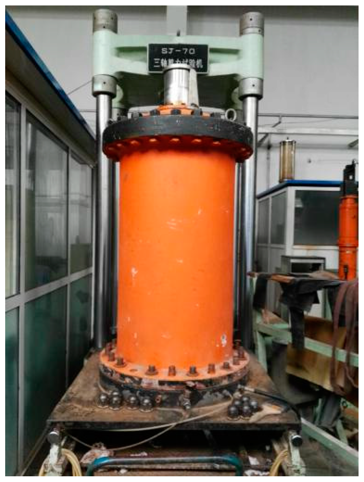
The triaxial shear tests under unconsolidated and undrained conditions for conditioned sandy pebble were conducted by using large triaxial shear apparatus (SJ-70, China Institute of Water Resources and Hydropower Research, Beijing, China), as shown in Figure 4. When making test samples, the prepared conditioned soil was compacted by means of vibration by five layers. The molded sample has a diameter of 300 mm, height of 700 mm, and wet density of 2 g/cm3. During tests, the confining pressure was set to 0.4 MPa, 0.6 MPa, and 0.8 MPa, successively, and the shear rate was maintained at 1 mm/min. Figure 5 records the measured stress–strain curves. Since no peak can be seen in the stress–strain curve, the corresponding point with strain of 15% is treated as failure point. Subsequently, Morh’s circles and their enveloping line are plotted in Figure 6, from which the total shear strength indexes are determined as cohesion and internal friction angle .
3. Geometric Model of the Particle Element
The particle element model mainly involves geometric model and physical model. As for the geometric model, it includes three aspects: particle shape, particle size distribution, and particle spatial arrangement.
3.1. Particle Shape
To take into consideration the angularity effect induced by irregular shape, the alternative approaches include exerting rolling resistance on single sphere and adopting nonspherical particles. So this paper involves two types of shape—basic sphere and cluster of particles—furthermore, the simulation result and computational cost of the two established models can be comparatively analyzed. Figure 7 shows the adopted geometry template of cluster, which is randomly selected for the irregular pebble. And the template is fitted with four same spheres (see Figure 7). It can be seen that the constructed cluster is nearly an ellipsoid, and the ratio of its polar radius, short equatorial radius, and long equatorial radius is 1:1.19:1.69.
3.2. Particle Size Distribution
Particle size distribution has certain effect on the macroscopic deformation and strength of bulk materials. Ideally, the particle size should be consistent with the substantial material. However, since the actual soil grains are generally too small, which will result in huge amount of particle elements and hence unacceptable computational cost, proper handling of the particle size is therefore necessary. It is generally accepted in the community that the simulation is aimed to investigate the macroscopic behavior of bulk materials instead of detailed interactions between particles. Thus, the particles of soil can be upscaled into surrogate particles which are much larger than the physical sizes of the grains in order to reduce the computational cost as long as a proper surrogate model can be found and validated.
From granulometric curve in Figure 1, it can be seen that the conditioned soil contains large amount of fine grains and are continuously distributed in numerous sizes. In order to reduce the particle number, the particle size is amplified here. Besides, since it is hardly possible to involve all particle sizes, only a few representative sizes are selected and herein the aperture diameters of the sieve meshes used in the sieving test are designated. Moreover, the large grains act as the main medium for force transmission in the soil mass, while most of the small grains only act as filler to fill the porous space. It can be concluded that omitting small particles has slight effect on the resultant mechanical response. So the original particle size is not only multiplied and discretized, but also truncated.
However, the determination of particle sizes and amplification factor should take into account computational cost, simulation accuracy, as well as opening size of shield machine. According to relevant experience, the number of particles should be controlled within 300,000. With single sphere model as example, Table 1 presents the particle number required for a soil box (24 m × 8 m × 2m) when adopting different size combinations and the corresponding minimum amplification factor to ensure an acceptable particle number. Additionally, the throughput capacity of the cutterhead and screw conveyor is also considerable. In view of the inner diameter of screw conveyor only 770 mm, the particle size cannot be too large: otherwise clogging and jamming accidents are easy to occur. On the premise of meeting the above two requirements and to model the material as realistically as possible, it is decided to magnify the particle 6 times and to select the size combination of 40 mm, 25 mm, and 20 mm. And, the particles of 240 mm, 150 mm, and 120 mm account for 10.82%, 9.02%, and 80.16% of the total mass, respectively.
3.3. Particle Arrangement
In order to embody the significant anisotropy and spatial variability of soil mass, the particles in this simulation are arranged by random function, and they are oriented randomly when generated.
4. Physical Model between Particles
4.1. Contact Components
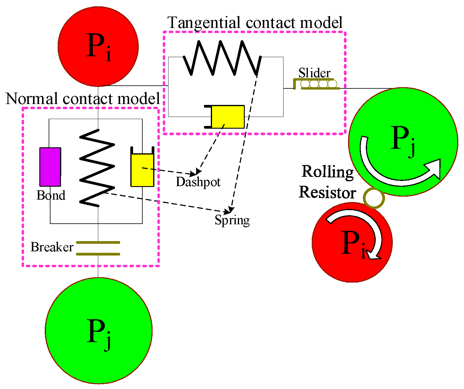
Compared with the natural sandy pebble, the cohesion among conditioned grains has been greatly enhanced under the action of foam and bentonite slurry. Thus cementitious interaction should be introduced in the contact model in addition to the standard contact action. In this study, the sphere and cluster employ the Hertz–Mindlin model (H-M) with the Johnson–Kendall–Roberts (JKR) cohesion model. The physical analogue characterized by several contact components for H-M with JKR cohesion model can be seen in Figure 8. Among them, the spring is used to simulate the elastic contact force between particles Pi and Pj The damper is a description of energy dissipation in the process of imperfect elastic collision. The frictional components include resistance devices to relative slide and rotation. The viscous components mainly provide resistance to tension, shear and torsion severally in the direction of normal, tangential and rotation. Those viscous components can simulate the viscous force exerted on pebble grains by foam and bentonite slurry. While the breaker implies the tension vanishes once the bonding between particles breaks.
4.2. Contact Constitutive Relation
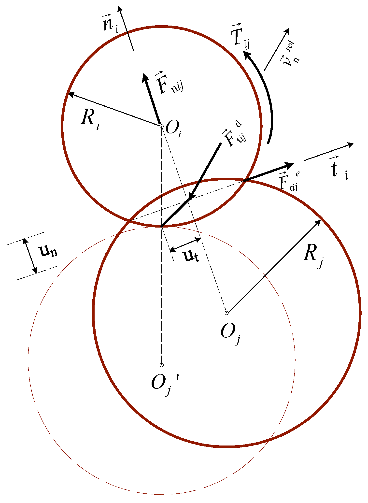
A schematic diagram of contact vectors in the H-M model can be found in Figure 9. In the model, the calculation of normal elastic force is based on Hertzian contact theory [29], while the tangential elastic force was derived by Mindlin and Deresiewicz [21,30]. As for the energy dissipation in the contact process, Tsuji et al. [31] proposed a nonlinear normal damping force and tangential damping force . Hence, the contact action exerted on particle by particle can be expressed as follows
where, and denote the normal and tangential overlap of particle and particle , respectively; is shear stiffness, ; denotes equivalent normal stiffness, ; , , , and denote Young’s modulus, radius, mass, and shear modulus of particles in contact, respectively; denotes damping coefficient, which is associated to the restitution coefficient by ; and and denote the normal and tangential components of relative speed of two particles, respectively.
The tangential force obeys Coulomb law of friction [32], that is to say if ( is friction force and denotes the coefficient of sliding friction), then slip occurs. While the rolling friction is accounted for by applying directional constant torque model [33], namely , where is the coefficient of rolling friction, is the distance from the mass center of particle to the contact point, denotes the unit vector of angular velocity.
To describe adhesive action, JKR theory enriched the Hertz–Mindlin model with normal cohesion force, and the normal elastic force is revised to [34]
where, denotes surface energy per unit of contact area, measured in J/m2; the relationship between coefficient and normal overlap can be expressed as .
5. Calibration of Model Parameters
5.1. Undetermined Parameters
The macroscopic and mesoscopic parameters in DEM model can be subdivided into three categories. The intrinsic parameters, including shear modulus , Poisson’s ratio , and density , are inherent attribute of material itself and irrelevant to the external factors. The H-M contact parameters include restitution coefficient , static friction coefficient , and rolling friction coefficient . The third category is about cohesion parameter and different model involves different cohesion parameters. JKR cohesion model only contains surface energy . Table 2 lists all of the involved materials and contact parameters. Among them, some are either measured or obtained from literature and the others need to be calibrated. So there are altogether three undetermined parameters (, , and ) in the H-M with JKR cohesion model.
5.2. Method
With the purpose of making the flow behavior and mechanical properties of the modeled soil consistent with the reality, the calibration procedures are as follows. First of all, we established the least squares support vector machine (LS-SVM) with unknown parameters as input variables and the slump value as output variable. Then generate 10,000 parameter combinations at random and predict their corresponding slump value with the constructed LS-SVM. Subsequently, use the parameters that can turn out a desired slump value to simulate the large-scale triaxial shear test. Among all the triaxial tests, the one resulting in smallest deviation of stress–strain curve from measured curve in laboratory is regarded as calibration result.
5.3. Calibration Process
5.3.1. Range of Parameters
Before the establishment of LS-SVM, the correlations between the slump value and three undetermined parameters, as well as the value range of each parameter are analyzed by single-variable method. Figure 10 shows the established discrete element models for slump test. Similarly, the slump cone has been enlarged 6 times with top diameter of 600 mm, bottom diameter of 1200 mm, and height of 1800 mm. In the simulation, the lifting speed is 0.36 m/s and the whole lifting process is completed in 5 s.
Figure 11 records the slump value against the surface energy in the cases of single sphere (a) and cluster (b) when and , successively. As is indicated in the figures, the slump value is in negative correlation to . It can be explained by (1) low surface energy: the mutual cohesion is rather weak and the interparticle forces cannot resist the particle weight, therefore the aggregation is easy to scatter into single particles, which makes for a large slump value (Figure 12a,e). (2) When the surface energy improves, the internal contact force is strong enough to resist gravity, thus the aggregation can deform continuously and displays good fluidity and plasticity as the actual conditioned soil. Consequently, the slump value is reduced (Figure 12b,f). (3) If the surface energy is excessively high, the soil presents poor fluidity thus leading to a small slump (Figure 12c,g). In addition, it can be seen from Figure 11 that the slump value is also negatively correlated to . This is because the strong rolling friction contributes to a strong interlocking action and makes it harder to deform.
Figure 13 shows the variation of slump value versus in six different scenarios of and (taking sphere model as example). It is obvious that no strict correlation exists between slump value and restitution coefficient . On the whole, the slump value increases as improves.
On the basis of literature research, the range of the restitution coefficient is set as , while the scope of the other two parameters are determined according to their correlation with the slump value. Figure 14a,b shows the slump value against rolling friction coefficient when respectively in the case of sphere and cluster. It can be concluded that once for sphere or for cluster, the slump value is less than 160mm regardless of the value of . It means even without cohesive force between particles, the frictional interaction is strong enough to resist the flow of soil. In such a situation, the slump value can no more meet the requirements. Therefore, the rolling friction coefficient should be set within 0.22 and 0.15, respectively, for sphere and cluster. Similarly, as shown in Figure 15, when and for sphere ( for cluster), the slump value cannot fall into the satisfactory range. So the reasonable scope of surface energy is for sphere and for cluster.
5.3.2. Parameter Sets with Satisfactory Fluidity
Then the LS-SVM that reflects the nonlinear relationship of slump value and three undetermined parameters can be established. As for training samples, some sets of unknown parameters are randomly generated within their respective range and the corresponding slumps are obtained through discrete element simulation. LS-SVR adopts a RBF kernel and its parameters are tuned by the GA-PSO collaborative algorithm. In the tuning process, the n-fold cross-validation error is chosen as a fitness function. For the sphere model, 440 training samples are collected altogether and n = 5. The parameters of LS-SVM are optimized as penalty parameter and kernel parameter . While in the cluster model, only 99 samples are collected and n is set as 9. And the optimization result is , . For the two cases, the comparison between the fitted values and numerically calculated values can be seen in Figure 16a,b. The resultant root mean square errors (RMSE) are 12.53 and 9.68, respectively, indicating a satisfactory degree of accuracy.
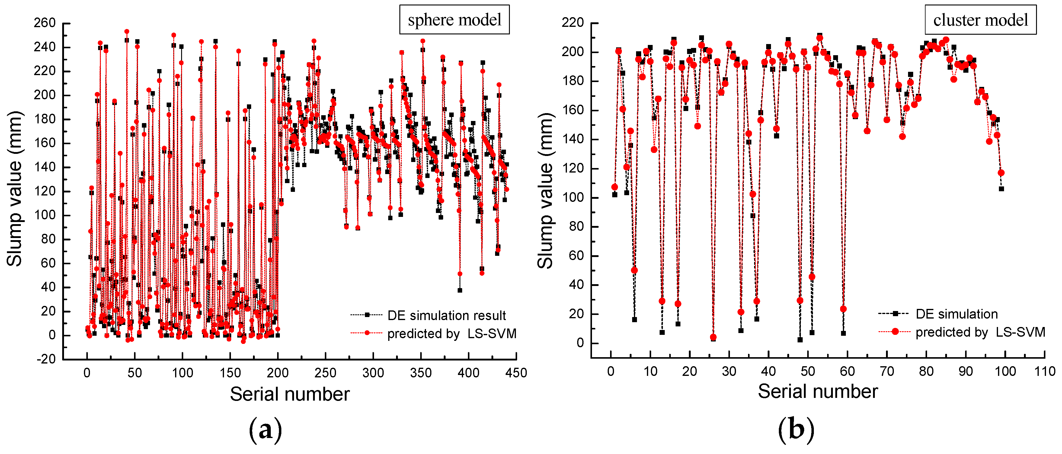
Based on the established slump prediction model, the parameter sets that can result in a desired slump can be found. Firstly, randomly generate 10,000 parameter sets and predict their corresponding slump value by the established LS-SVM. Since the on-site measured slump ranges from 175 mm to 180 mm, and with a consideration of fitting error, the samples resulting in a slump between 170 mm and 185 mm are further checked by discrete element simulation. If the simulated slump can fall into the range of 175 to 180 mm, the corresponding parameter set is considered to be able to meet the requirement for fluidity. By regression analysis with LS-SVM, 86 (72) out of 10,000 sets of parameters get a satisfactory slump value in the case of sphere (cluster); Figure 17 shows comparison between fitted values and numerically calculated values of the 86 (72) sets, among which 22 (26) calculated values range from 175 mm to 180 mm. In addition, Figure 17 also indicates that the constructed LS-SVMs have satisfactory generalization ability and prediction accuracy.
5.3.3. Strength Required Parameter Set
DE simulations of triaxial shear test are carried out successively with previously found parameter sets adopted, and the one with result closest to the experimental result is regarded as desired parameter set. Since the calculated static earth pressure at tunnel face ranges from 66.39 kPa to 92.98 kPa, and measured soil pressure at the bulkhead fluctuates between 30 kPa and 80 kPa, the soil inside shield chamber works in a low-pressure state. Therefore, the parameter sets are evaluated by the stress–strain curve measured under confining pressure of 0.4 MPa. Figure 18 presents the established discrete element models for the simulation of triaxial test. In the simulation, the confining pressure is realized by exerting body force on peripheral particles via developing custom plugin programmed in C++; the body force equals to the product of confining pressure and contact area between particle and boundary. According to Hu [7], the contact radius of particle and geometry can be approximately taken as particle radius.
In the single sphere case, the 22 test specimens fall into three groups according to simulation result. The first group involves the 12th, 14th, 19th, 20th, 21st, and 22nd specimens. As for the six specimens, the measured stresses constantly remain zero except for the beginning of loading. This is because their surface energy is too low. With weak cohesive force between particles, the soil specimens have insufficient strength and self-stability. Therefore collapse occurs under the disturbance of axial load. The evolution of the 12th specimen along with loading can be seen in Figure 19.
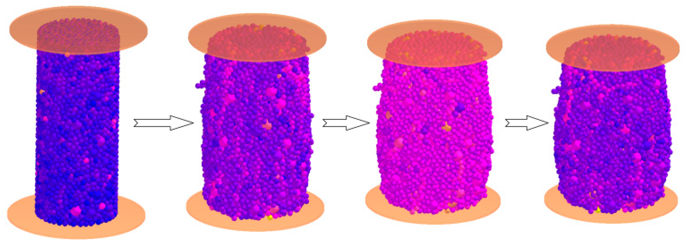
Whereas, the second group consists of the 2nd, 3rd, 4th, 6th, 9th, 11th, 15th, 16th, and 18th specimens. Compared with the first group, the nine soil specimens have developed some intensity because of the improved cohesive force between particles. Their stress–strain curves measured under the confining pressure of 0.4 MPa are shown in Figure 20. It can be seen that both the shape and value of the curves deviate greatly from the result of laboratory test (see Figure 4). Figure 21 records the evolution of the 2nd specimen during shear process. Obviously, the soil specimen expands continuously, leading to an ongoing reduce in interlocking induced shear resistance. Once the cohesive force and friction force are not enough to resist external force, local damage begins to occur on the specimen. Along with loading, the damage area gradually gets larger and only a part of soil specimen works in the end.
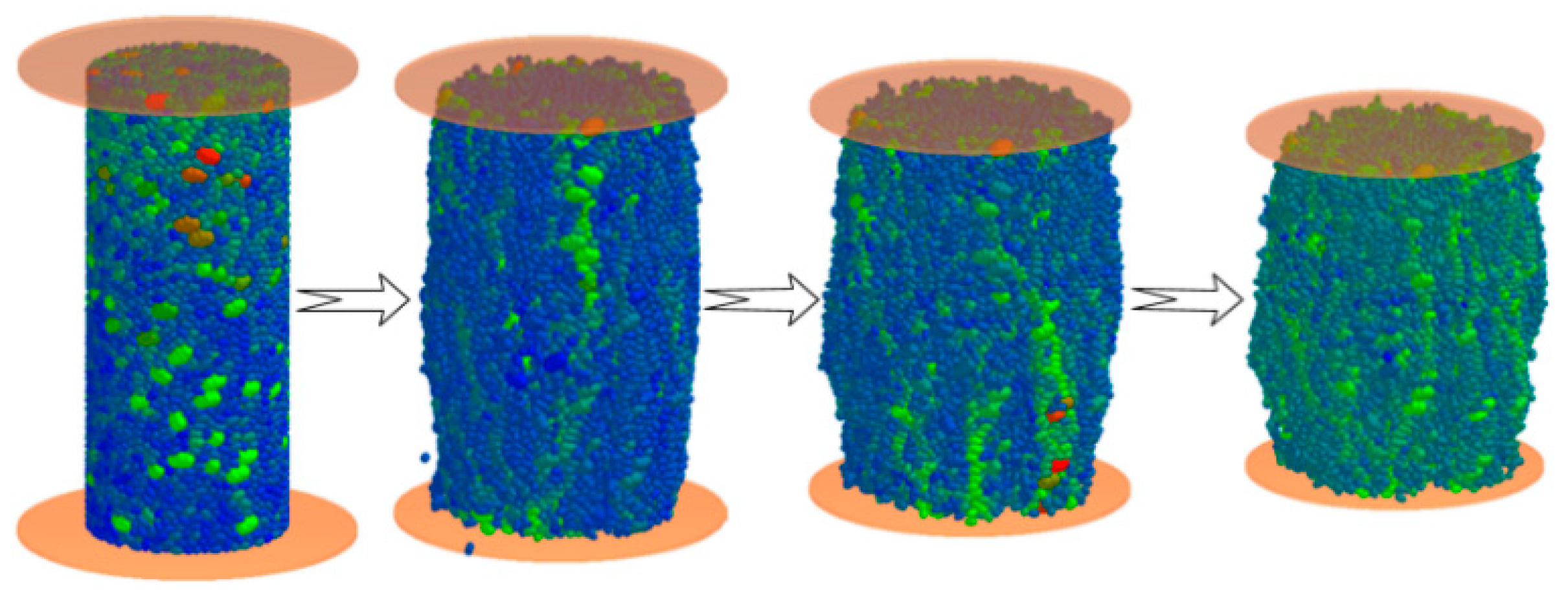
The third group, including the 1st, 5th, 7th, 8th, 10th, 13th, and 17th specimens, behaves similarly with the actual soil in laboratory. The stress–strain curves of the seven specimens (see Figure 22) generally experience three stages, namely initial stage, strain hardening stage and strain softening stage (or constant strain stage). At the beginning of the second stage, the deviatoric stress rises rapidly because the closely packed particles must overcome a strong interlocking resistance for shear dislocation, but the duration is short before shear dilation occurs. When the volume of specimen increases, the soil becomes loose, resulting in weakened interlocking effect between particles and thus a reduction in growth speed of stress. Then a peak, namely peak strength, can be seen in the curve with certain expanded specimen volume. Along with the increasing shear load, the curve turns into the third stage. In this stage, the specimen keeps expanding, but the shear strength decreases. Finally, the curve fluctuates at residual strength as a result of continuous stress relaxation. The residual strength is mainly shear resistance provided by sliding friction and rolling friction. Figure 23 shows the variation of the first specimen in the shear process. As the shear load increases, the specimen appears to undergo bulging deformation. It can be concluded from Figure 22; Figure 23 that discrete element simulation can embody the nonlinearity, plasticity, strain softening, and shear dilatancy of granular material. There are two possible reasons why the laboratory test cannot reflect the strain softening and shear dilatancy: (1) With improved gradation and vibration method adopted when making sample, the conditioned soil grains are closely arranged, therefore strong interlocking exists among grains. (2) Besides, the sample was wrapped with a rubber film when testing. Constrained by the rubber film, the soil cannot deform easily. Moreover, Figure 22 also shows that the 13th simulation has the most similar stress–strain curve to the laboratory test. Therefore, a decent set of parameters is found as , , and . In this way, the established discrete element model is almost consistent with the actual soil both with respect to strength property and fluidity.
Similarly, the 26 cluster specimens fall into three groups. Figure 24 shows the stress–strain curves of the specimens in the third group, and Figure 25 presents the evolution of the 2nd specimen. So for the cluster model, the desired parameters are , , and .
From the above analysis it is notable that when cluster is adopted, lower values for rolling friction coefficient and surface energy are required to obtain a good match between the experiment and DEM simulation. This is because there exists additional strength gained from interlocking action due to the irregular shape of the cluster. Besides, in the cluster case the CPU processing time for slump test and triaxial shear test are respectively 144 min and 1235 min, which are 4.97 times and 3.68 times higher than that in the sphere case.
6. Conclusions
This paper constructed two particle element models for conditioned sandy pebble. To take the shape effect into account, rolling resistance was exerted on the single sphere or the single sphere was replaced by the cluster of particles. Based on a laboratory test and DEM simulation of the slump test and large-scale triaxial test, the undetermined contact parameters in two models were calibrated by virtue of LS-SVR. Through comparative analysis, the following conclusions have been obtained.
- (1)
- Because of the angularity of the nonspherical grains, there exists strong interlocking between clusters. So in the cluster model, relatively smaller rolling friction coefficient and surface energy are required.
- (2)
- Since the model parameters are properly calibrated, the two established particle models both can well describe the strength property and fluidity of the actual soil. However, the cluster model takes ~4 times longer than the sphere model to execute the simulation.
It is worth noting that calibrating parameters by intelligent algorithm is still a time consuming task. There is an urgent need to conduct further research into multifunctional testing device for direct measurement of material parameters. An uncertainty analysis as done in [36,37,38] might be helpful.
Author Contributions
P.C. is responsible for the model setup and computational. X.Z. validated and checked the model. H.Z. is the PI of the project and supervised the work. Y.L. analysed the results and data.
Funding
The authors gratefully acknowledge the supports from the National Natural Science Foundation of China (Grant No. 41672360), Science and Technology Commission of Shanghai Municipality (Grant No. 17DZ1203800), and Shanghai Shentong Metro Group Co., Ltd. (Grant No. 17DZ1203804).
Conflicts of Interest
The authors declare no conflict of interest.
References
- Zhang, P.; Jin, L.; Du, X.; Lu, D. Computational homogenization for mechanical properties of sand cobble stratum based on fractal theory. Eng. Geol. 2018, 232, 82–93. [Google Scholar] [CrossRef]
- Yagiz, S. Brief notes on the influence of shape and percentage of gravel on the shear strength of sand and gravel mixtures. Bull. Eng. Geol. Environ. 2001, 60, 321–333. [Google Scholar] [CrossRef]
- Maynar, M.J.M.; Rodríguez, L.E.M. Discrete numerical model for analysis of earth pressure balance tunnel excavation. J. Geotech. Geoenviron. Eng. 2005, 131, 1234–1242. [Google Scholar] [CrossRef]
- Rabczuk, T.; Belytschko, T. A three dimensional large deformation meshfree method for arbitrary evolving cracks. Comput. Methods Appl. Mech. Eng. 2007, 196, 2777–2799. [Google Scholar] [CrossRef]
- Rabczuk, T.; Belytschko, T. Cracking particles: a simplified meshfree method for arbitrary evolving cracks. Int. J. Numer. Methods Eng. 2004, 61, 2316–2343. [Google Scholar] [CrossRef]
- Rabczuk, T.; Gracie, R.; Song, J.H.; Belytschko, T. Immersed particle method for fluid-structure interaction. Int. J. Numer. Methods Eng. 2010, 81, 48–71. [Google Scholar] [CrossRef]
- Amiri, F.; Anitescu, C.; Arroyo, M.; Bordas, S.; Rabczuk, T. XLME interpolants, a seamless bridge between XFEM and enriched meshless methods. Comput. Mech. 2014, 53, 45–57. [Google Scholar] [CrossRef]
- Rabczuk, T.; Bordas, S.; Zi, G. On three-dimensional modelling of crack growth using partition of unity methods. Comput. Struct. 2010, 88, 1391–1411. [Google Scholar] [CrossRef]
- Rabczuk, T.; Zi, G.; Bordas, S.; Nguyen-Xuan, H. A simple and robust three-dimensional cracking-particle method without enrichment. Comput. Methods Appl. Mech. Eng. 2010, 199, 2437–2455. [Google Scholar] [CrossRef]
- Areias, P.; Cesar de Sa, J.; Rabczuk, T.; Camanho, P.P.; Reinoso, J. Effective 2D and 3D crack propagation with local mesh refinement and the screened Poisson equation. Eng. Fract. Mech. 2018, 189, 339–360. [Google Scholar] [CrossRef]
- Areias, P.; Rabczuk, T. Steiner-point free edge cutting of tetrahedral meshes with applications in fracture. Finite Elem. Anal. Des. 2017, 132, 27–41. [Google Scholar] [CrossRef]
- Areias, P.; Rabczuk, T.; Msekh, M. Phase-field analysis of finite-strain plates and shells including element subdivision. Comput. Methods Appl. Mech. Eng. 2016, 312, 322–350. [Google Scholar] [CrossRef]
- Areias, P.; Msekh, M.A.; Rabczuk, T. Damage and fracture algorithm using the screened Poisson equation and local remeshing. Eng. Fract. Mech. 2016, 158, 116–143. [Google Scholar] [CrossRef]
- Areias, P.; Rabczuk, T.; Dias-da-Costa, D. Element-wise fracture algorithm based on rotation of edges. Eng. Fract. Mech. 2013, 110, 113–137. [Google Scholar] [CrossRef] [Green Version]
- Ren, H.; Zhuang, X.; Rabczuk, T. Dual-horizon peridynamics: A stable solution to varying horizons. Comput. Methods Appl. Mech. Eng. 2017, 318, 762–782. [Google Scholar] [CrossRef] [Green Version]
- Ren, H.; Zhuang, X.; Cai, Y.; Rabczuk, T. Dual-Horizon Peridynamics. Int. J. Numer. Methods Eng. 2016, 108, 1451–1476. [Google Scholar] [CrossRef]
- Talebi, H.; Silani, M.; Rabczuk, T. Concurrent Multiscale Modelling of Three Dimensional Crack and Dislocation Propagation. Adv. Eng. Softw. 2015, 80, 82–92. [Google Scholar] [CrossRef]
- Talebi, H.; Silani, M.; Bordas, S.; Kerfriden, P.; Rabczuk, T. A Computational Library for Multiscale Modelling of Material Failure. Comput. Mech. 2014, 53, 1047–1071. [Google Scholar] [CrossRef]
- Budarapu, P.; Gracie, R.; Bordas, S.; Rabczuk, T. An adaptive multiscale method for quasi-static crack growth. Comput. Mech. 2014, 53, 1129–1148. [Google Scholar] [CrossRef]
- Budarapu, P.; Gracie, R.; Shih-Wei, Y.; Zhuang, X.; Rabczuk, T. Efficient Coarse Graining in Multiscale Modeling of Fracture. Theor. Appl. Fract. Mech. 2014, 69, 126–143. [Google Scholar] [CrossRef]
- Mindlin, R.D. Compliance of elastic bodies in contact. J. Appl. Mech. 1949, 16, 259–268. [Google Scholar]
- Tavares, L.M.; King, R.P. Single-particle fracture under impact loading. Int. J. Miner. Process. 1998, 54, 1–28. [Google Scholar] [CrossRef]
- Mishra, B.K.; Murty, C. On the determination of contact parameters for realistic DEM simulations of ball mills. Powder Technol. 2001, 115, 290–297. [Google Scholar] [CrossRef]
- Jayasundara, C.T.; Yang, R.Y.; Yu, A.B.; Rubenstein, J. Effects of disc rotation speed and media loading on particle flow and grinding performance in a horizontal stirred mill. Int. J. Miner. Process. 2010, 96, 27–35. [Google Scholar] [CrossRef]
- Rosenkranz, S.; Breitung-Faes, S.; Kwade, A. Experimental investigations and modelling of the ball motion in planetary ball mills. Powder Technol. 2011, 212, 224–230. [Google Scholar] [CrossRef]
- Piechatzek, T.; Kwade, A. DEM based characterization of stirred media mills. In Proceedings of the European Symposium on Comminution, Espoo, Finland, 15–18 September 2009. [Google Scholar]
- Quist, J.C.E. Device for calibrating of DEM contact model parameters. In Proceedings of the EDEM Conference, Edinburgh, UK, 5–7 April 2011. [Google Scholar]
- Li, C.Q.; Liu, T.W.; Zhang, H.Y. Back-analysis on micromechanical parameters of soil mass using BP neural network. J. Eng. Geol. 2015, 23, 609–615. (In Chinese) [Google Scholar]
- Hertz, H. On the contact of elastic solids. J. Fur Die Reine Und Angew. Math. 1882, 92, 156–171. [Google Scholar]
- Mindlin, R.D.; Deresiewicz, H. Elastic spheres in contact under varying oblique forces. ASME J. Appl. Mech. 1953, 20, 327–344. [Google Scholar]
- Tsuji, Y.; Tanaka, T.; Ishida, T. Lagrangian numerical simulation of plug flow of cohesionless particles in a horizontal pipe. Powder Technol. 1992, 71, 239–250. [Google Scholar] [CrossRef]
- Cundall, P.A.; Strack, O.D.L. A discrete numerical method for granular assemblies. Geotechnique 1979, 29, 47–65. [Google Scholar] [CrossRef]
- Sakaguchi, E.; Ozaki, E.; Igarashi, T. Plugging of the flow of granular materials during the discharge from a silo. Int. J. Mod. Phys. B 1993, 7, 1949–1963. [Google Scholar] [CrossRef]
- Johnson, K.L.; Kendal, K.; Roberts, A.D. Surface energy and the contact of elastic solids. Proc. R. Soc. A 1971, 324, 301–313. [Google Scholar] [CrossRef]
- Hu, M.; Xu, G.Y.; Hu, S.B. Study of equivalent elastic modulus of sand gravel soil with Eshelby tensor and Mori-Tanaka equivalent method. Rock Soil Mech. 2013, 34, 1437–1442. (In Chinese) [Google Scholar]
- Vu-Bac, N.; Lahmer, T.; Zhuang, X.; Nguyen-Thoi, T.; Rabczuk, T. A software framework for probabilistic sensitivity analysis for computationally expensive models. Adv. Eng. Softw. 2016, 100, 19–31. [Google Scholar] [CrossRef]
- Hamdia, K.; Zhuang, X.; Silani, M.; He, P.; Rabczuk, T. Stochastic analysis of the fracture toughness of polymeric nanoparticle composites using polynomial chaos expansions. Int. J. Fract. 2017, 206, 215–227. [Google Scholar] [CrossRef]
- Hamdia, K.; Zhuang, X.; Alajlan, N.; Rabczuk, T. Sensitivity and uncertainty analyses for exoelectric nanostructures. Comput. Methods Appl. Mech. Eng. 2018, 337, 95–109. [Google Scholar] [CrossRef]
Figure 1.
Granulometric curves of natural soil and conditioned soil.

Figure 2.
Slump test at the construction site.
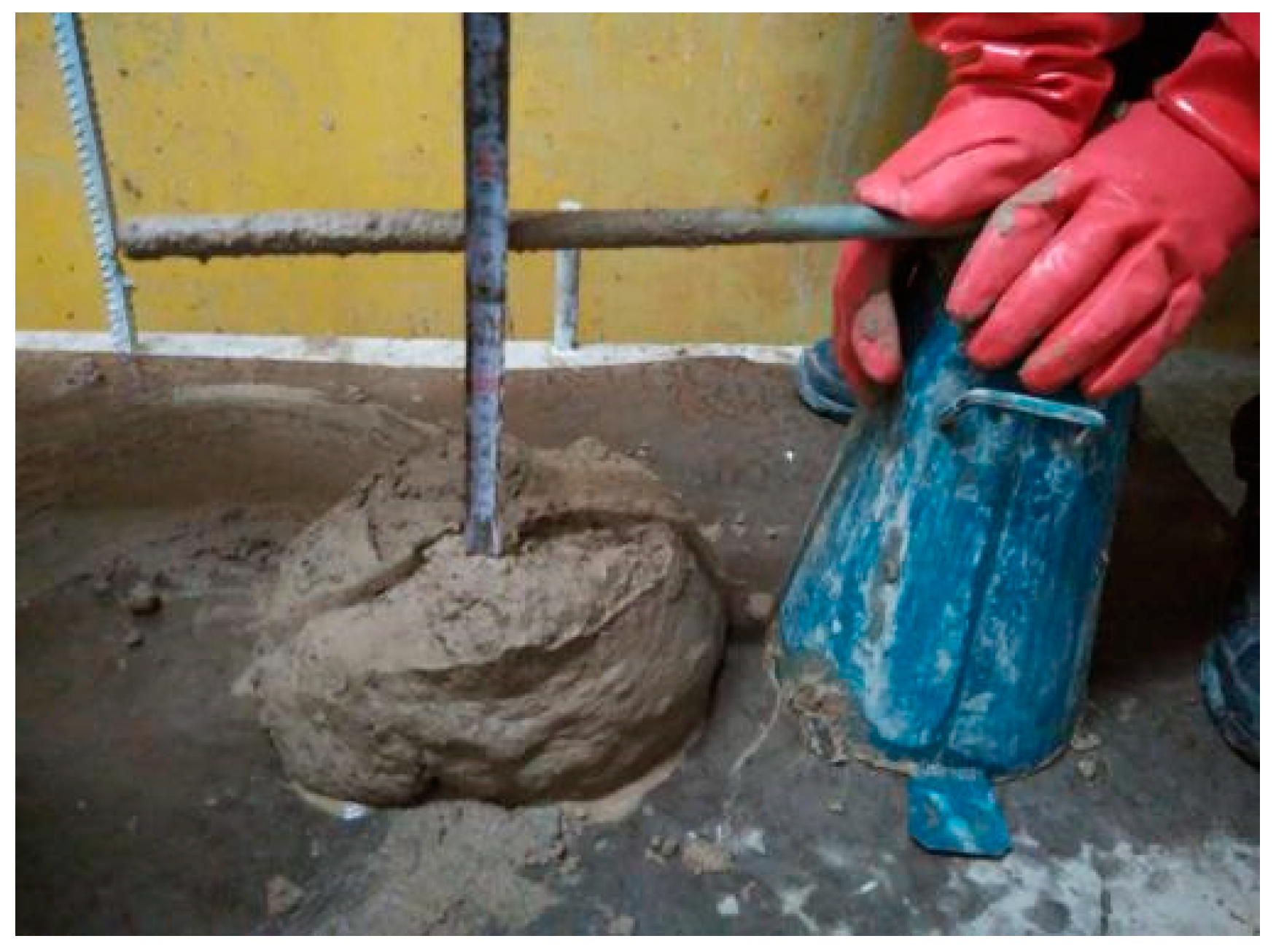
Figure 3.
The slump value of soil from muck discharging vehicle.
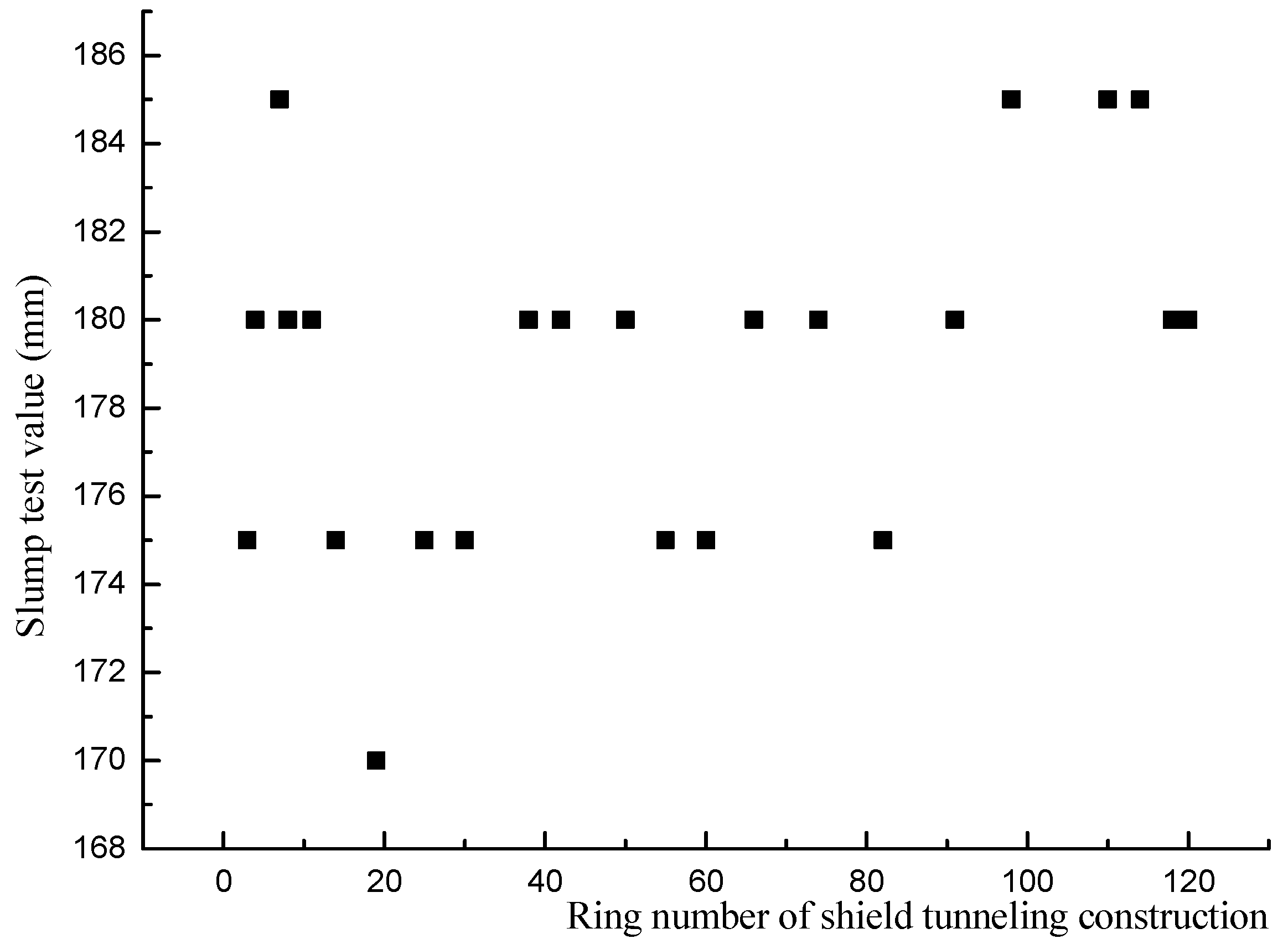
Figure 4.
Large-scale triaxial shear test.

Figure 5.
Stress–strain curves.
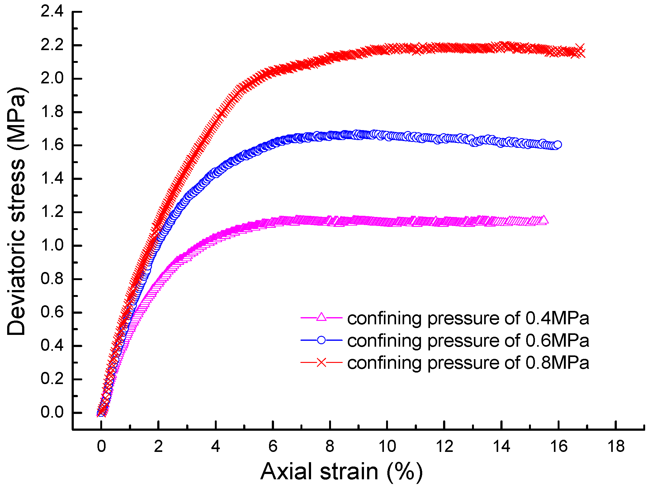
Figure 6.
Morh’s circles and enveloping line of conditioned sandy pebble.
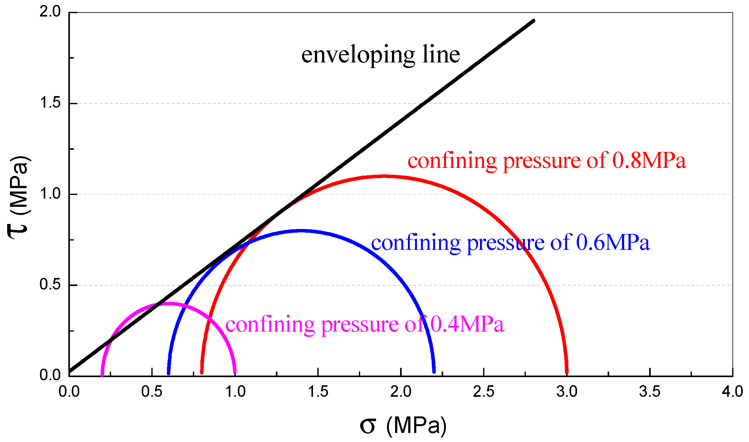
Figure 7.
3D geometry of realistic irregular pebble to the left and cluster model to the right.
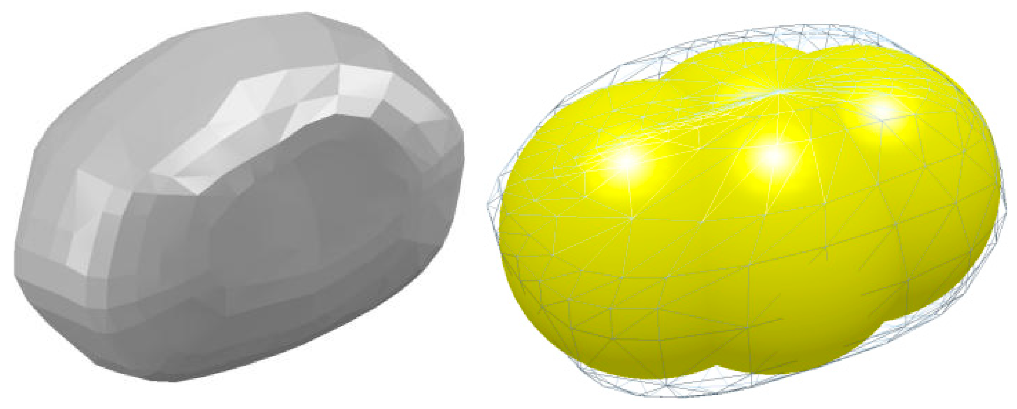
Figure 8.
Physical contact models of conditioned soil.

Figure 9.
Schematic representation of Hertz–Mindlin contact model.

Figure 10.
Slump test model of sphere (a) and cluster (b).
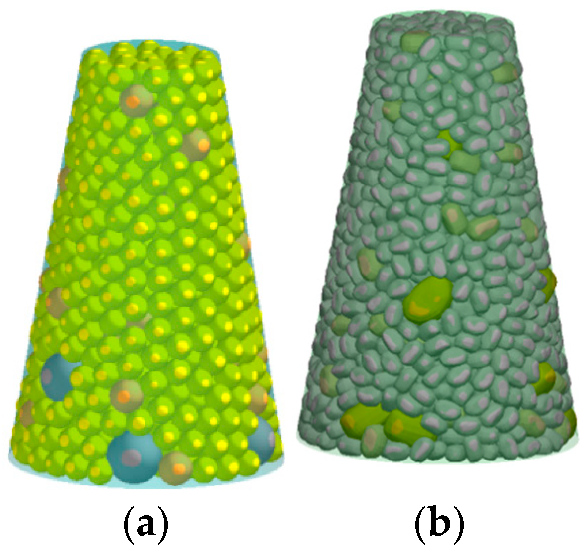
Figure 11.
The variation of slump value versus surface energy: (a) sphere model and (b) cluster model.
Figure 11.
The variation of slump value versus surface energy: (a) sphere model and (b) cluster model.
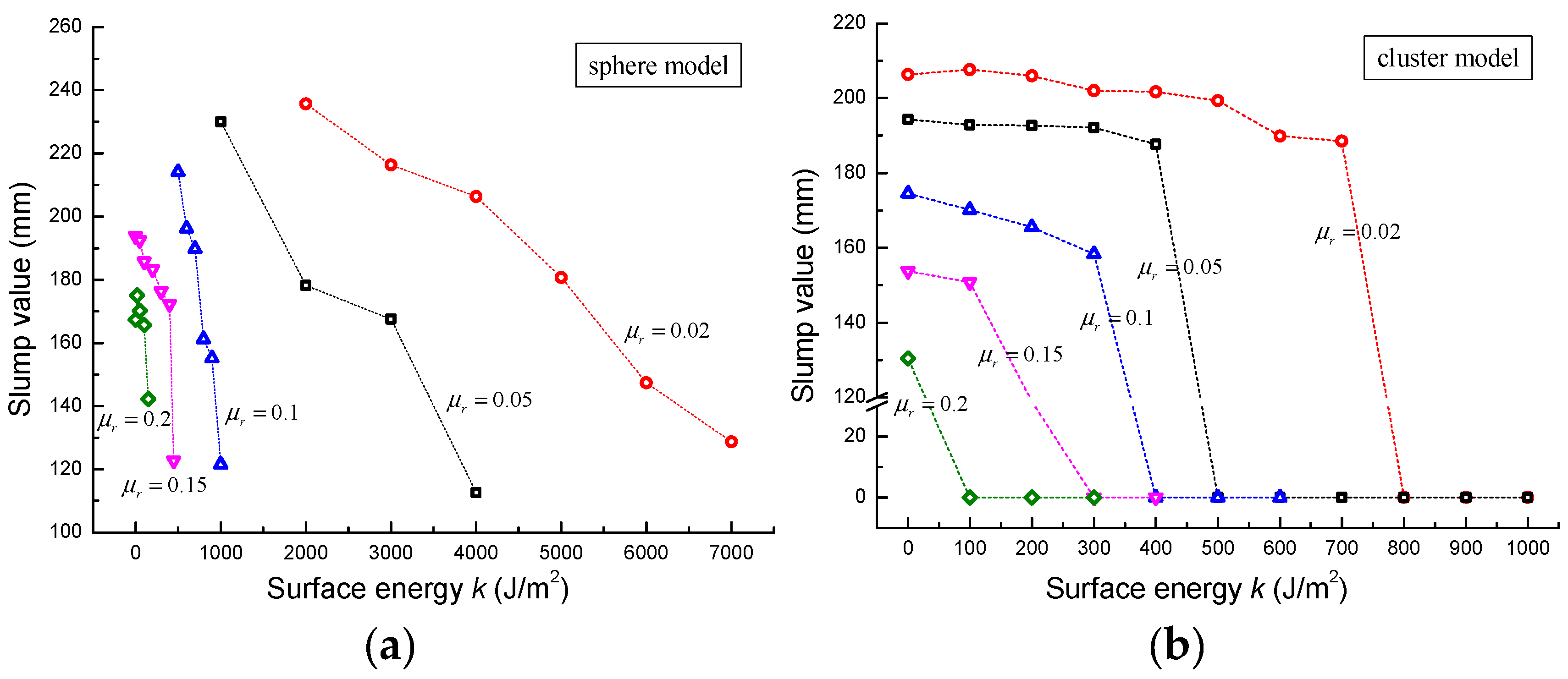
Figure 12.
The simulation result of slump test: (a–c) sphere model and (e–g) cluster model.
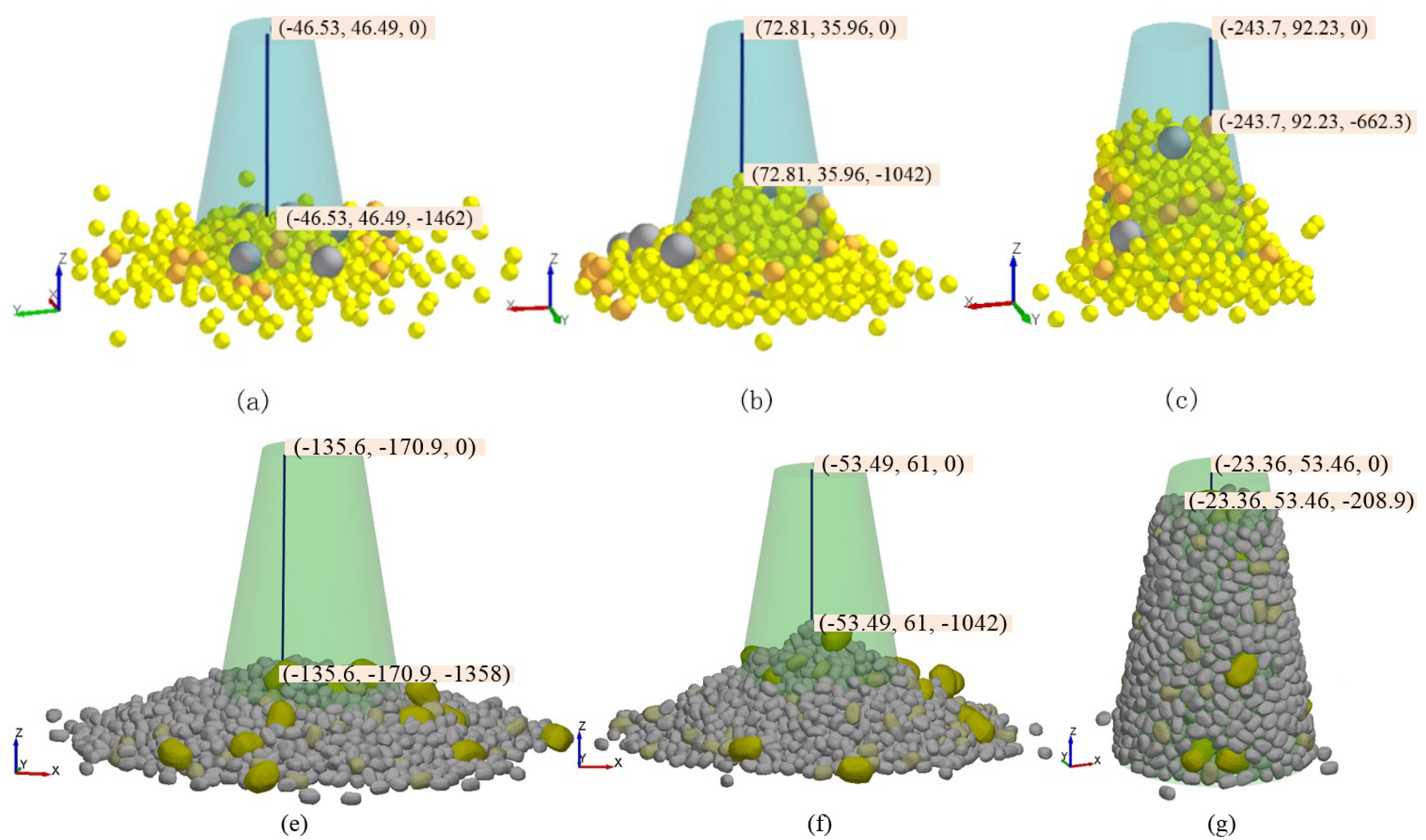
Figure 13.
The slump value against restitution coefficient.
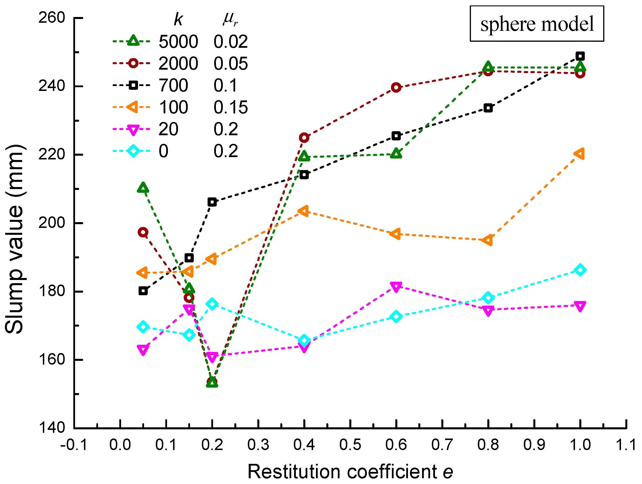
Figure 14.
The slump value against rolling friction coefficient (): (a) sphere model and (b) cluster model.
Figure 14.
The slump value against rolling friction coefficient (): (a) sphere model and (b) cluster model.
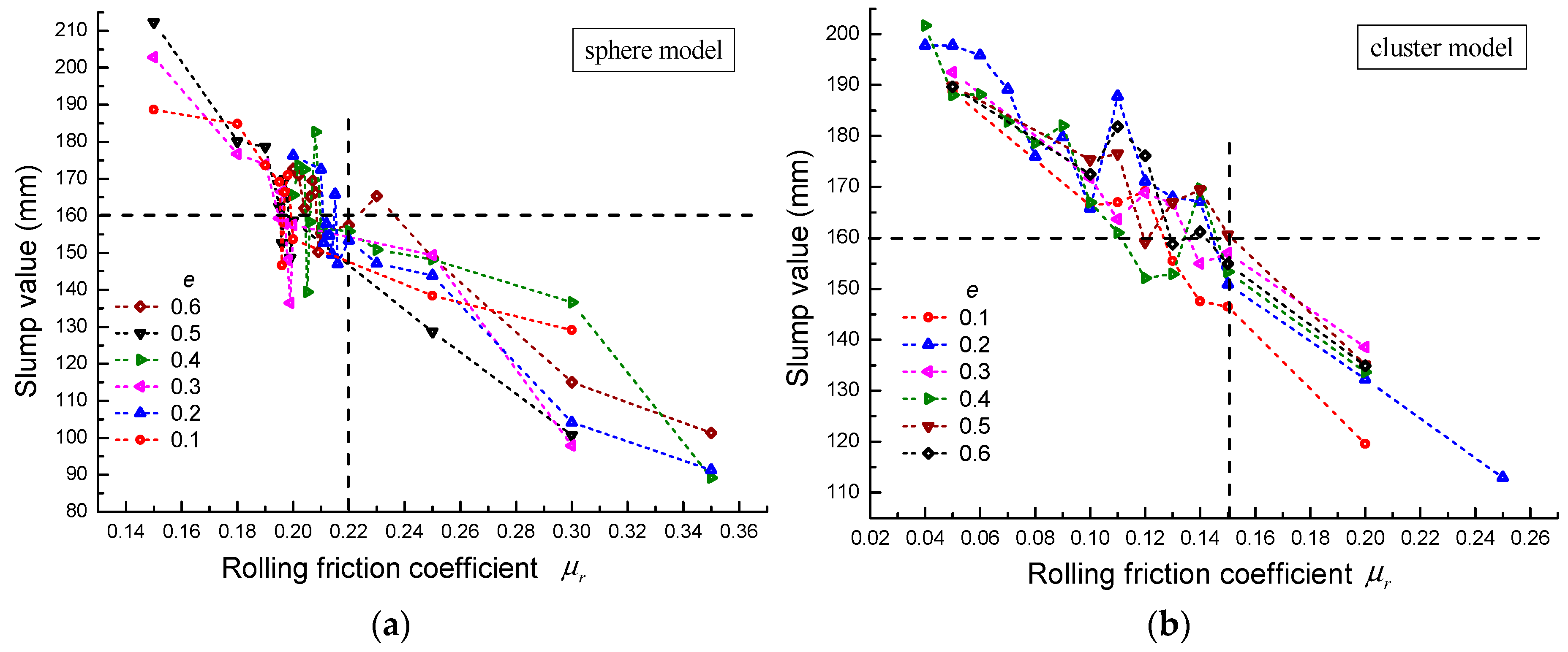
Figure 15.
The slump value against surface energy (): (a) sphere model and (b) cluster model.
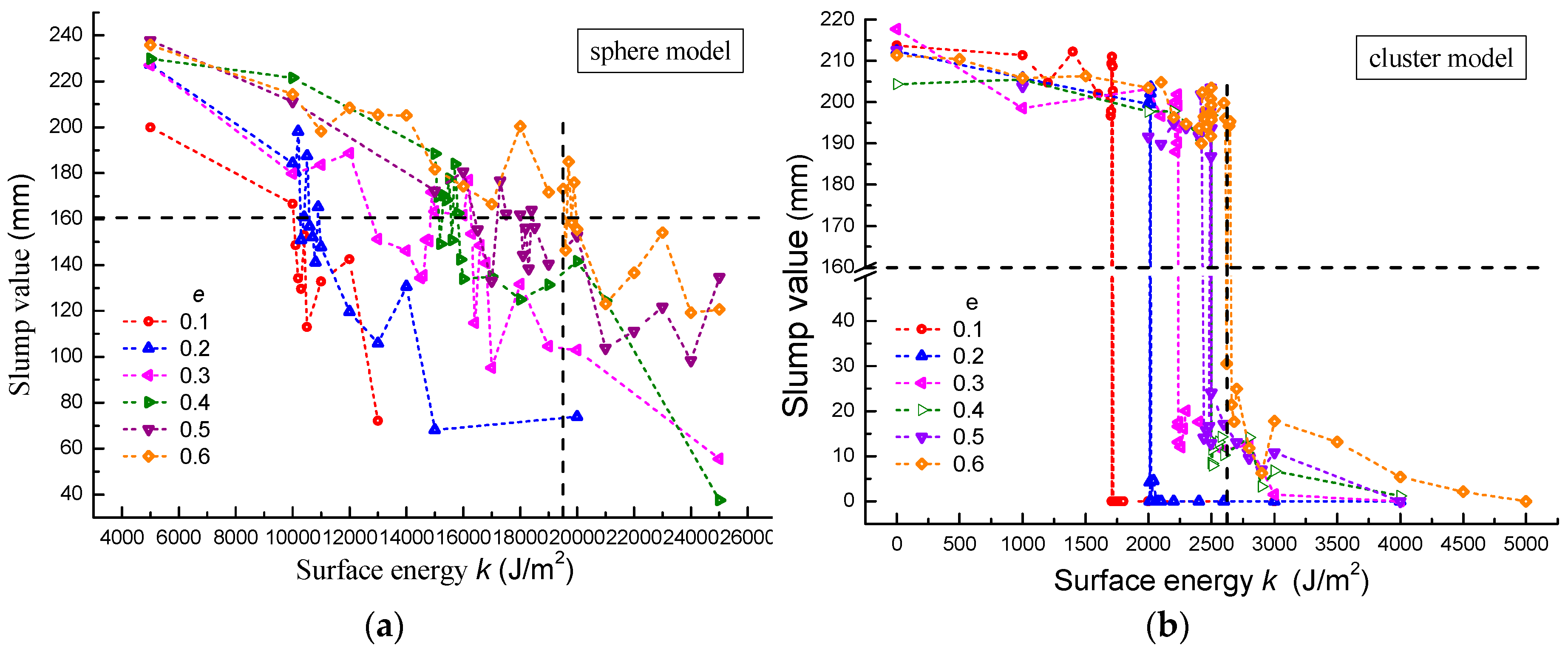
Figure 16.
Comparison of fitted values and discrete element method (DEM) result: (a) sphere model and (b) cluster model.
Figure 16.
Comparison of fitted values and discrete element method (DEM) result: (a) sphere model and (b) cluster model.

Figure 17.
Comparison of fitted values and numerically calculated values: (a) sphere model; and (b) cluster model.
Figure 17.
Comparison of fitted values and numerically calculated values: (a) sphere model; and (b) cluster model.

Figure 18.
Discrete element models for triaxial test.
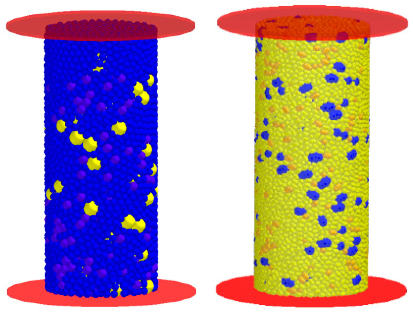
Figure 19.
The evolution of the 12th specimen as loading.
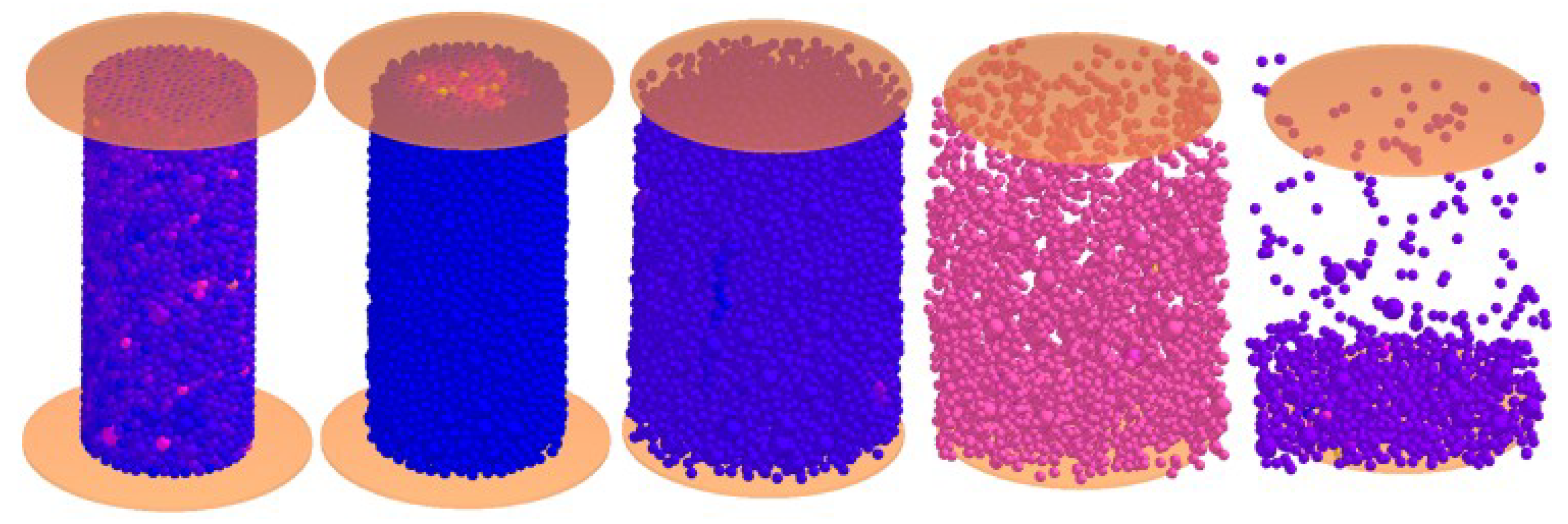
Figure 20.
The stress–strain curve of specimens in the second group.
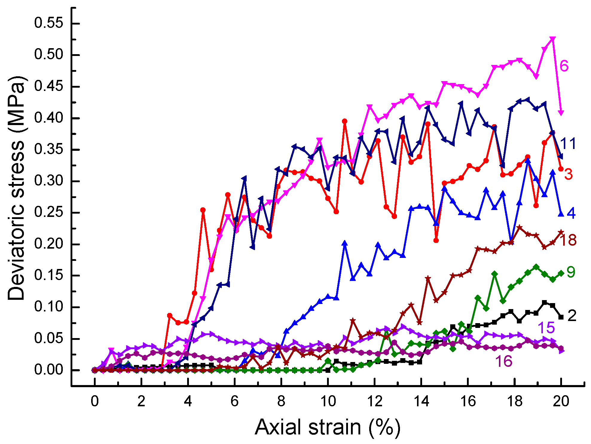
Figure 21.
The evolution of the 2nd specimen as loading.
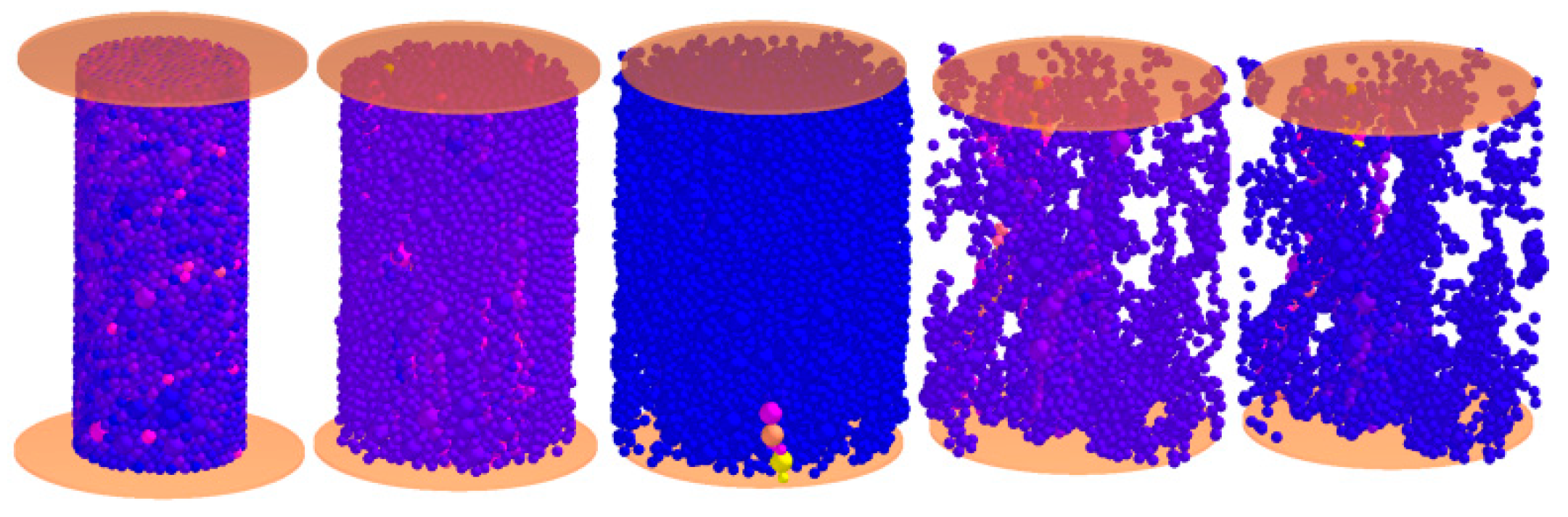
Figure 22.
The stress–strain curve of specimens in the third group.
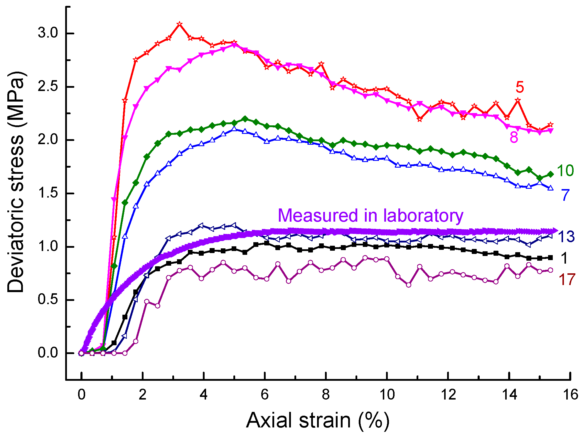
Figure 23.
The evolution of the 1st specimen.

Figure 24.
The stress–strain curve of cluster specimens.
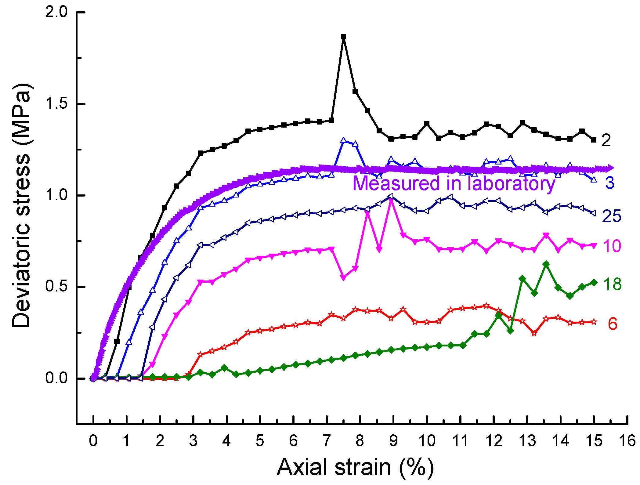
Figure 25.
The evolution of the 2nd specimen.

Table 1.
The required particle number when adopting different size combinations.
| Combination of Particle Size (mm) | Particle Number (×106) | Minimum Amplification Factor | Particle Number after Amplification |
|---|---|---|---|
| 40-25-20-16-10-5 | 2219 | 20 | 277,375 |
| 40-25-20-16-10 | 358.4 | 11 | 269,271 |
| 40-25-20-16 | 107.1 | 8 | 209,180 |
| 40-25-20 | 58.487 | 6 | 270,773 |
| 40-25 | 31.924 | 5 | 255,392 |
Table 2.
The input parameters for the simulation model.
| Input S | Unit | Value | Comment |
|---|---|---|---|
| Material Parameter | |||
| Density ρ | kg/m3 | 2700 | Measured by overflow method |
| Poisson’s ratio ν | n/a | 0.15 | Hu et al. (2013) [35] |
| Yong’s modulus E | MPa | 5 × 10⁴ | Hu et al. (2013) [35] |
| Shear modulus G | MPa | 2.17 × 10⁴ | |
| H-M Contact parameter | |||
| Restitution coefficient e | n/a | To be calibrated | |
| Static friction coefficient μs | n/a | 0.6891 | |
| Rolling friction coefficient μr | n/a | To be calibrated | |
| Cohesion parameter (JKR model) | |||
| Surface energy k | J/m2 | To be calibrated | |
© 2019 by the authors. Licensee MDPI, Basel, Switzerland. This article is an open access article distributed under the terms and conditions of the Creative Commons Attribution (CC BY) license (http://creativecommons.org/licenses/by/4.0/).
Share and Cite
MDPI and ACS Style
Cheng, P.; Zhuang, X.; Zhu, H.; Li, Y. The Construction of Equivalent Particle Element Models for Conditioned Sandy Pebble. Appl. Sci. 2019, 9, 1137. https://doi.org/10.3390/app9061137
AMA Style
Cheng P, Zhuang X, Zhu H, Li Y. The Construction of Equivalent Particle Element Models for Conditioned Sandy Pebble. Applied Sciences. 2019; 9(6):1137. https://doi.org/10.3390/app9061137
Chicago/Turabian StyleCheng, Panpan, Xiaoying Zhuang, Hehua Zhu, and Yuanhai Li. 2019. "The Construction of Equivalent Particle Element Models for Conditioned Sandy Pebble" Applied Sciences 9, no. 6: 1137. https://doi.org/10.3390/app9061137
Note that from the first issue of 2016, this journal uses article numbers instead of page numbers. See further details here.